Relic Black Holes and Type 2 Quasars

Abstract

We follow the evolution of the Black Hole mass function in the assumption that mass accretion onto a massive BH is the powering mechanism of AGN activity. With reasonable assumptions suggested by current knowledge, it is possible to reproduce the Black Hole mass function derived from local bulges. In particular it is found that the majority of the mass in relic Black Holes was produced during AGN activity and that the ratio between obscured and unobscured quasars is between 1 and 2, much lower than required by synthesis models of the X-ray background.

Osservatorio Astrofisico di Arcetri, Largo Fermi 5, 50125 Firenze, Italy

1. Introduction

It has long been suspected that the most luminous Active Galactic Nuclei (AGN) are powered by accretion of matter onto massive black holes (BH). This belief, combined with the observed evolution of the space-density of AGN suggests that massive BHs should be present in local galaxies as relics of past activity. Indeed, the current observational evidence indicates that most, possibly all, luminous galaxies host a massive BH at their centres and its mass correlates with the luminosity and stellar velocity dispersion of the bulge in which it resides (e.g. Richstone et al. 1998, Ferrarese & Merritt 2000). Soltan (1982) and Chokshi & Turner (1992) derived the local mass density in relic BHs, $\rho_{\rm BH}$ , expected from past activity using optical number counts of AGNs. More recently, Fabian & Iwasawa (1999) estimated $\rho_{\rm BH}$  from the energy density of the hard X-Ray Background (XRB) and this value is in agreement with the observed local BH density derived by Merritt & Ferrarese (2001) using the BH-mass vs Bulge-mass relation. However it seems that the AGNs found in optical and soft X-ray surveys are not enough to account for the local $\rho_{\rm BH}$  and this fact prompted Fabian & Iwasawa to talk about ”obscured accretion”, i.e. obscured AGN activity. The existence of obscured AGNs (the so-called ”type 2” objects) is required to account for the XRB spectrum with integrated emission from AGNs (e.g. Gilli, Salvati & Hasinger 2001 and references therein): the ratio between type 2 and unobscured type 1 objects (hereafter ${\rm R}_{2-1}$) is usually in the range 4-10, implying that both optical and Xray surveys are missing a large fraction of the AGN population. With a completely independent argument, the missing Lyman edge in blue quasars implies that ${\rm R}_{2-1}$ is at least $\geq 0.5$ (Maiolino et al. 2001). Locally, low luminosity obscured AGNs are well known (Seyfert 2 galaxies) and in the ratio of about 4:1 with respect to type 1 objects (Maiolino & Rieke 1995). However, at higher redshifts few type 2 quasars (high luminosity objects) are known, a number which is largely insufficient to account for the spectral shape of the XRB. What is the relationship between type 2 AGNs and massive black holes? The arguments based on $\rho_{\rm BH}$  indicates that some obscured AGNs must exist in order to account for the fossil mass but nothing can be told about the luminosity of these obscured objects: are many low luminosity AGNs needed or could fewer high luminosity quasars suffice? Is it really true that AGN activity can explain the local BHs, not only globally, but also in terms of their mass distribution? This paper will try to answer these questions by comparing the local BH mass function (BHMF) expected from AGN activity with the local BHMF inferred from galaxy bulges. Throughout this paper we assume $H_{\circ}=70$km/s/Mpc^-1, $\Omega_{\rm M}=1$ and $\Omega_{\Lambda}=0$.

Figure 1.: (a) AGN luminosity function at $z=1.0$ (solid line) and $z=2.5$ (dashed line). This is obtained by combining the XLF by Gilli, Salvati & Hasinger 2001 (low $L$) and the OLF by Boyle et al. 2000 (high $L$). (b) Local BH Mass Function (solid line). The uncertainties are represented by the gray area. The dashed line is the BHMF obtained assuming that $\sigma_{\mbox{$x$}}=0$.

2. The continuity equation

We consider the continuity equation which regulates the time evolution of the BH mass function with the Small & Blandford (1992) formalism. If $N(M,t)$ is the BH mass function ($\mbox{$N(M,t)$}{\rm d}M$ is the number of BHs per unit comoving volume (Mpc^-3) at cosmic time $t$), the continuity equation can be written as:

$$\frac{\partial\mbox{$N(M,t)$}}{\partial t}+\frac{\partial}{\partial M}\left(\mbox{$N(M,t)$}<\mbox{$\mbox{$\dot{M}$}(M,t)$}>\right)=S(M,t)$$ (1)

where $<\mbox{$\mbox{$\dot{M}$}(M,t)$}>$ is the ”average” accretion rate and $S(M,t)$ is the source function. As in Small & Blandford (1992) we assume that a massive BH is ”born” when its mass is $M\geq M_{\rm min}$ and that no BH is created or destroyed (i.e. we neglect any merging process). With these assumptions the source function is simply $S(M,t)=S_{\circ}\delta(M-M_{\rm min})$ where $\delta$ is the Dirac delta function. If AGNs are powered by accretion onto BHs, we can relate the AGN Luminosity Function $\phi(L,t)$ ($\mbox{$\phi(L,t)$}{\rm dln}L$ is the number of AGNs per unit comoving volume (Mpc^-3) at cosmic time $t$) to the BH mass function

$$\phi(L,t)\mbox{${\rm d\ln}L$}=\delta(M,t)N(M,t)\mbox{${\rm d}M$}$$ (2)

where $\delta(M,t)$ is the fraction of BHs with mass M active at time $t$. If a BH is accreting at a fraction $\lambda$ of the Eddington rate its emitted luminosity is then $L=\lambda Mc^{2}/t_{E}=\varepsilon\mbox{$\dot{M}$}c^{2}$ where $t_{E}$ is the Eddington time, $\varepsilon$ is the accretion efficiency and $\dot{M}$ is the accretion rate. Since $<\mbox{$\mbox{$\dot{M}$}(M,t)$}>=\delta(M,t)\mbox{$\mbox{$\dot{M}$}(M,t)$}$, we can write:

$$\mbox{$N(M,t)$}<\mbox{$\mbox{$\dot{M}$}(M,t)$}>=\frac{\lambda}{\varepsilon t_{E}}\left[\phi(L,t)\right]_{L=\lambda\frac{Mc^{2}}{t_{E}}}$$ (3)

$$\frac{\partial\mbox{$N(M,t)$}}{\partial t}=-\frac{c^{2}\lambda^{2}}{\varepsilon t_{E}^{2}}\left[\frac{\partial\phi(L,t)}{\partial L}\right]_{L=\lambda\frac{Mc^{2}}{t_{E}}}$$ (4)

which can be easily integrated given the AGN luminosity function AND the initial conditions. When $\lambda$ is dependent on $M$ the equation is more complex but still easily solvable. As initial conditions, we assume that at a given redshift $z_{\circ}$ ($\mbox{$t_{\circ}$}=t(\mbox{$z_{\circ}$})$) ALL Black Holes are active, i.e. that $\delta(M,t(\mbox{$z_{\circ}$}))=1$. The only constraint is that $\delta(M,t)=\phi(L,t)/MN(M,t)\leq 1$.

A fundamental ingredient is the AGN luminosity function (LF) expressed in terms of the total AGN luminosity, $L$. We first consider the LF of optically selected quasars (OLF in the B band; Boyle et al. 2000) and the LF of soft X-ray selected AGNs (XLF in 0.5-2 keV band; Gilli et al. 2001, it represents only unabsorbed AGNs and is derived using the XLF by Miyaji, Hasinger & Schmidt 2000). Both LFs consider only type 1 (unobscured) AGNs. In principle the LF in one spectral band should be enough to obtain $\phi(L,t)$ but in this paper we consider more instructive to combine the above LFs using Boyle’s LF to describe high $L$ AGNs and Gilli’s one to describe low $L$ AGNs. A more refined treatment will be presented elsewhere. The AGN luminosity function for type 1 objects is plotted in Fig. 1a at two redshift values. We have assumed $L/L_{\rm X}=30$, for low L objects and $L/\mbox{$\nu_{\rm B}$}L_{\mbox{$\nu_{\rm B}$}}=15$ as typical of quasars (e.g. Elvis et al. 1994).

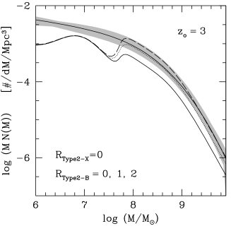
Figure 2.: (a) Local BH mass function from galaxy bulges (solid line in grey area) compared with BH mass function obtained considering only type 1 AGNs (solid line). The dotted lines are the contributions from low and high $L$ AGNs. The dot-dashed line is the BH mass function at the redshift $z_{\circ}$=3 when all BHs were active. The dashed line represents the BHMF from AGN activity assuming that only 10% of the BHs were active at $z_{\circ}$=5. (b)The contribution from high $L$ AGNs is computed for ${\rm R}_{2-1,B}$=0 (solid line), 1 (dotted line), 2 (dashed line).

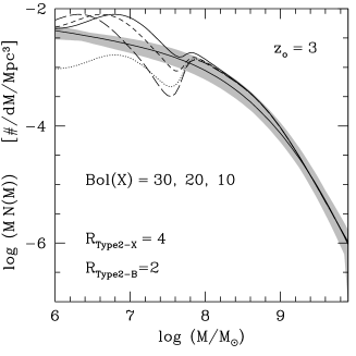
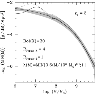
Figure 3.: (a) BHMF from AGN activity computed with ${\rm R}_{2-1,X}$=4 for $L/L_{\rm X}=$ 30 (solid line), 20 (short-dashed line), 10 (long-dashed line). The dotted line represent the model with ${\rm R}_{2-1,X}$=0. (b) The dotted and solid lines represent models with $L/L_{\rm X}=30$, $L/\mbox{$\nu_{\rm B}$}L_{\mbox{$\nu_{\rm B}$}}=15$ and ${\rm R}_{2-1,X}$=4. In the model represented by the dotted line all AGNs are emitting at their Eddington luminosity, while with the solid line AGNs are emitting at a fraction of their Eddington luminosity which depends on $M$ as specified in the figure. For this model ${\rm R}_{2-1,B}$=1.

3. The local BH mass function

To estimate the local BH mass function we follow the method by Salucci et al. (1999). The BHMF is derived from the Galaxy LF through the following steps: (1) we consider the LF of galaxies in the B band divided by morphological type (Folkes et al. 1999); (2) for each morphological type we derive the LF of bulges applying the bulge/disk ratio by Simien & de Vaucouleurs (1985); (3) we obtain the mass function of bulges using the mass-to-light ratio by Fukugita, Hogan, & Peebles (1998); (4) we convolve the bulge mass function with the probability distribution of the ratio $\mbox{$M_{\rm BH}$}/\mbox{$M_{\rm Bulge}$}$ to obtain the BH mass function. An important assumption in the last point is that the observed scatter in the $M_{\rm BH}$- $M_{\rm Bulge}$ relation is real and not due to observational uncertainties. We then assume a gaussian probability distribution $P(\log{\mbox{$x$}})$ ($\mbox{$x$}=\mbox{$M_{\rm BH}$}/\mbox{$M_{\rm Bulge}$}$) with $<\log\mbox{$x$}>=-2.93$ and $\sigma_{\mbox{$x$}}=0.45$ as derived by Merritt & Ferrarese (2001). The BHMF is presented in Fig. 1b and the ”grey” region represent an error estimate on the BH mass function obtained by varying the parameters used in each of the above steps. The BHMF has $\mbox{ $\rho_{\rm BH}$ }=(5\pm 2)\mbox{$\times 10^{5}$}\mbox{${\rm M}_{\odot}$}\mbox{${\rm\,Mpc}$}\mbox{${}^{-3}$}$ and this value is in agreement with $\mbox{ $\rho_{\rm BH}$ }=(3\div 6)\mbox{$\times 10^{5}$}\mbox{${\rm M}_{\odot}$}\mbox{${\rm\,Mpc}$}\mbox{${}^{-3}$}$ obtained by Fabian & Iwasawa (1999) and Salucci et al. (1999) from the hard XRB.

4. Model Results

Model results are shown in Fig. 2a. The solid line in the grey area is the BH mass function derived from the galaxy mass function as indicated in the previous section. The solid line is the BH mass function expected from type 1 AGNs only with a starting redshift of $\mbox{$z_{\circ}$}=3$. The starting redshift at which we make the assumption of $\delta(M,\mbox{$t_{\circ}$})=1$ (or alternatively the redshift at which we select the active BHs whose evolution we will follow) is not important for the final results. Indeed the dotted line representing the BHMF obtained assuming $z_{\circ}$=5 and $\delta=0.1$, is not significantly different from the one with $z_{\circ}$=3 and $\delta=1$. The only constraint is that $\mbox{$z_{\circ}$}>z_{\rm max}$, the redshift of maximum AGN activity. From Fig. 2a it is clear that Optical QSOs (high $L$ AGNs) produce black holes with masses $\mbox{$M_{\rm BH}$}>\mbox{$10^{8}$}\mbox{${\rm M}_{\odot}$}$ while X-ray AGNs (low $L$ AGNs) produce the lower mass ones. Moreover, comparing the BHMF obtained from AGN activity at $z=0$ with the one at $z_{\circ}$ it can be clearly seen that BH masses are produced during the AGN activity: this is the main reason why the results are little sensitive to the initial conditions. The model presented in the figure has ${\rm R}_{2-1}$=0, i.e. it considers only unobscured AGNs. Thus it is not unexpected to derive a low $\rho_{\rm BH}$ =1.8$\times 10^{5}$${\rm M}_{\odot}$${\rm\,Mpc}$^-3. Let’s first consider the high $L$ AGNs. It is not yet clear if type 2 quasars exist or not or what is their ratio ${\rm R}_{2-1}$ relative to type 1 objects. The comparison between the ”observed” local BHMF with the one deduced from AGN activity can yield a constraint on ${\rm R}_{2-1}$. From Fig. 2b, $1<\mbox{${\rm R}_{2-1}$}<2$ is required to match the local BHMF in absolute level (the slope is nicely reproduced). Correspondingly $\mbox{ $\rho_{\rm BH}$ }=3.2\div 4.6\mbox{$\times 10^{5}$}\mbox{$M_{\rm BH}$}\mbox{${\rm\,Mpc}$}\mbox{${}^{-3}$}$. Let’s now focus on the low $L$ AGNs. The existence of low $L$ type 2 AGNs is well know and the local ratio is ${\rm R}_{2-1}$=4 (e.g. Maiolino & Rieke 1995). As shown in Fig. 3, with that ratio the local BHMF at low masses ($\mbox{$M_{\rm BH}$}<\mbox{$10^{8}$}\mbox{${\rm M}_{\odot}$}$) is overproduced. A change in the bolometric correction does not improve the situation because the BHMF is just shifted along the M axis. A possible solution to this problem is that low luminosity AGNs are not emitting at the Eddington Luminosity (Fig. 3a), a possibility also considered in other works (e.g. Salucci et al. 1999 and references therein), and indeed, apart for some ”wiggles”, the BHMF is now well reproduced. One must keep in mind that this might also mean that there are some problems with the AGN luminosity functions at low luminosities or that the $M_{\rm BH}$-$M_{\rm Bulge}$ relation is different at low masses.

5. Summary and Conclusions

We have used the continuity equation to follow the evolution of the BH mass function in the assumption that mass accretion onto a BH is the powering mechanism of AGN activity. AGNs accrete at a fraction of their Eddington luminosity and at a starting redshift $z_{\circ}$ all BHs were active. By comparing the expected BHMF with the one derived from local galaxy luminosity functions we can make the following conclusions. (1) The majority of the mass of a local BH was produced during AGN activity. (2) Quasar activity was responsible for the growth of BHs with $M>\mbox{$10^{8}$}\mbox{${\rm M}_{\odot}$}$. (3) The final results are not sensitive to the value of the redshift $z_{\circ}$ at which all BH were active. (4) The ratio between type 2 and type 1 quasars is $\mbox{${\rm R}_{2-1}$}\simeq 1-2$, i.e. $\simeq 30\%-50\%$ of $\rho_{\rm BH}$  is made by type 2 QSOs. (5) The required ${\rm R}_{2-1,B}$ can be reduced if we assume that $L<L_{Eddington}$ or $\varepsilon<0.1$. In any case it is clear that (a) ${\rm R}_{2-1,B}$ is much lower than the $4-10$ value required to fit the XRB and (b) no small efficiencies are required to explain the local BHMF. (6) $\mbox{${\rm R}_{2-1,X}$}>0$ gives a problem at low masses overpredicting the number of relic BHs. This could indicate that either $L<L_{Eddington}$ at low luminosities or that there might be uncertainties on the BHMF and/or the AGN LF at low M and L. (7) No merging of BHs is required by our model.

The main conclusion of this work is that with ”reasonable” assumptions, compatible with current knowledge, mass accretion onto massive BH during AGN activity can explain the local BH mass function both in shape and normalization. There is not much room for a large ($R>>1$) population of high luminosity obscured AGNs (i.e. type 2 quasars).

References

Boyle, B.J., et al. 2000, MNRAS, 317, 1014

Chokshi, A., & Turner, E.L. 1992, MNRAS, 259, 421

Elvis, M., et al. 1994, ApJS, 95, 1

Fabian, A.C., & Iwasawa, K. 1999, MNRAS, 303, L34

Ferrarese, L., & Merritt, D. 2000, ApJ, 539, L9

Folkes, S., et al. 1999, MNRAS, 308, 459

Fukugita, M., Hogan, C.J., & Peebles, P.J.E. 1998, ApJ, 503, 518

Gilli, R., Salvati, M., & Hasinger, G. 2001, A&A, 366, 407

Macchetto, F., et al. 1997, ApJ, 489, 579

Maiolino, R., & Rieke, G.H. 1995, ApJ, 454, 95

Maiolino, R., Salvati, M., Marconi, A., & Antonucci, R. 2001, A&A, 375, 25

Marconi, A., et al. 2001, ApJ, 549, 915

Merritt, D., & Ferrarese, L. 2001, MNRAS, 320, L30

Miyaji, T., Hasinger, G., & Schmidt, M. 2000, 353, 25

Richstone, D. et al. 1998, Nature, 395, 14

Salucci, P., et al. 1999, MNRAS, 307, 637

Simien, F., & de Vaucouleurs, G. 1985, ApJ, 302, 564

Small, T.A., & Blandford, R.D. 1982, MNRAS, 259, 725

Soltan, A. 1982, MNRAS, 200, 115