On the properties of massive Population III stars and metal-free stellar populations

see below

Abstract

We present realistic models for massive Population III stars and stellar populations based on non-LTE model atmospheres, recent stellar evolution tracks and up-to-date evolutionary synthesis models, with the aim to study their spectral properties, including their dependence on age, star formation history, and IMF.

A comparison of plane parallel non-LTE model atmospheres and comoving frame calculations shows that even in the presence of some putative weak mass loss, the ionising spectra of metal-free populations differ little or negligibly from those obtained using plane parallel non-LTE models. As already discussed by Tumlinson & Shull (2000), the main salient property of Pop III stars is their increased ionising flux, especially in the He⁺ continuum ($>$ 54 eV).

The main result obtained for individual Pop III stars is the following: Due to their redward evolution off the zero age main sequence (ZAMS) the spectral hardness measured by the He⁺/H ionising flux is decreased by a factor $\sim$ 2 when averaged over their lifetime. If such stars would suffer strong mass loss, their spectral appearance could, however, remain similar to that of their ZAMS position.

The main results regarding integrated stellar populations are:

• For young bursts and the case of a constant SFR, nebular continuous emission — neglected in previous studies — dominates the spectrum redward of Lyman-$\alpha$ if the escape fraction of ionising photons out of the considered region is small or negligible. In consequence predicted emission line equivalent widths are considerably smaller than found in earlier studies, whereas the detection of the continuum is eased. Nebular line and continuous emission strongly affect the broad band photometric properties of Pop III objects.

• Due to the redward stellar evolution and short lifetimes of the most massive stars, the hardness of the ionising spectrum decreases rapidly, leading to the disappearance of the characteristic He ii recombination lines after $\sim$ 3 Myr in instantaneous bursts.

• He ii $\lambda$1640, H$\alpha$ (and other) line luminosities usable as indicators of the star formation rate are given for the case of a constant SFR. For obvious reasons such indicators depend strongly on the IMF.

• Due to an increased photon production and reduced metal yields, the relative efficiency of ionising photon energy to heavy element rest mass production, $\eta$, of metal-poor and metal-free populations is increased by factors of $\sim$ 4 to 18 with respect to solar metallicity and for “standard” IMFs.

• The lowest values of $\eta\sim$ 1.6 – 2.2 % are obtained for IMFs exclusively populated with high mass stars (M_low $\ga$ 50 M_⊙). If correct, the yields dominated by pair creation SNae then predict large overabundances of O/C and Si/C compared to solar abundance ratios.

Detailed results are given in tabular form and as fit formulae for easy implementation in other calculations. The predicted spectra will be used to study the detectability of Pop III galaxies and to derive optimal search strategies for such objects.

1 Introduction

Important advances have been made in recent years on the modeling of the first stars and galaxies forming out of pristine matter — so called Population III (Pop III) objects — in the early Universe (see e.g. the proceedings of Weiss et al. 2000 and Umemura & Susa 2001). Among the questions addressed (see also the reviews of Loeb & Barkana 2001 and Barkana & Loeb 2001) are the star formation process and the initial mass function (IMF) of the first stars (Tegmark et al. 1997, Abel et al. 1998, 2000, Bromm et al. 1999, Nakamura & Umemura 1999, 2001, Omukai & Palla 2001), their effect of energy injection and supernovae (SN) (MacLow & Ferrara 1999, Ciardi et al. 2000), their role on cosmic reionisation (Haiman & Loeb 1997, Gnedin & Ostriker 1997, Tumlinson & Shull 2000, Cojazzi et al. 2000, Ciardi et al. 2001), metal enrichment of the IGM and other signatures of early chemical evolution (Ferrara et al. 2000, Abia et al. 2001), and dust formation (Todini & Ferrara 2000).

Extensive sets of recent stellar evolution and nucleosynthesis calculations for zero metallicity stars covering a wide range of stellar masses have also become available recently (Marigo et al. 2000, Feijóo 1999, Desjacques 2000, Woosley & Weaver 1995, Heger et al. 2000, 2001, Umeda et al. 2000).

Tumlinson & Shull (2000, hereafter TS00) have recently pointed out the exceptionally strong He⁺ ionising flux of massive ($M\ga$ 40 M_⊙) Pop III stars, which must be a natural consequence of their compactness, i.e. high effective temperatures, and non-LTE effects in their atmospheres increasing the flux in the ionising continua. As a consequence strong He ii recombination lines such as He ii $\lambda$1640 or He ii $\lambda$4686 are expected; together with AGN a rather unique feature of metal-free stellar populations, as discussed by TS00 and Tumlinson et al. (2001, hereafter TGS01). Instead of assuming a “standard” Population I like Salpeter IMF and “normal” stellar masses up to 100 M_⊙ as TS00, Bromm et al. (2001) have considered stars with masses larger than 300 M_⊙, which may form according to some recent hydrodynamical models (Abel et al. 1998, Bromm et al. 1999, Nakamura & Umemura 2001). An even stronger ionising flux and stronger H and He ii emission lines was found.

Some strong simplifying assumptions are, however, made in the calculations of TS00, TGS01, and Bromm et al. (2001).

• All stars are assumed to be on the zero age main sequence, i.e. stellar evolution proceeding generally to cooler temperatures is neglected .

• Bromm et al. (2001) take the hardness of the stellar spectrum of the hottest (1000 M_⊙) star as representative for all stars with masses down to 300 M_⊙. This leads in particular to an overestimate of the He ii recombination line luminosities.

• None of the studies include nebular continuous emission, which cannot be neglected for metal-poor objects with such strong ionising fluxes. This process increases significantly the total continuum flux at wavelengths redward of Lyman-$\alpha$ and leads in turn to reduced emission line equivalent widths.

• A single, fixed, IMF is considered only by TS00 and TGS01. In view of the uncertainties on this quantity it appears useful to explore a wider range of IMFs.

The models presented here relax all the above assumptions and allow the exploration of a wide parameter space in terms of stellar tracks (including also alternate tracks with strong mass loss), IMF, and star formation history (instantaneous bursts or constant star formation rate (SFR)). For this aim we provide in particular the main results in tabulated form and as fit formulae.

First we examine the influence of several poorly constrained physical processes (mass loss, non coherent electron scattering etc.) on the predicted stellar fluxes of Pop III stars using non-LTE atmosphere models. Combined with metal-free stellar tracks these predictions are then introduced to our evolutionary synthesis code (Schaerer & Vacca 1998) updated to calculate the nebular properties (H and He emission lines and nebular continuum) for metal-free gas. In this manner we examine the properties of both individual Pop III stars and integrated stellar populations.

Calculations of the relative photon to metal production of stellar populations (e.g. Madau & Shull 1996) have proven useful for a variety of studies ranging from estimates of the stellar contribution to the UV background radiation (Madau & Shull 1996), over studies of metals in the IGM, to SN rates in the early Universe and their detectability (Miralda-Escudé & Rees 1997). To improve on such calculations based on solar metallicity models we also calculate the heavy element production from metal-poor and metal-free populations including contributions from type II SN and possible pair creation SN from very massive stars (cf. Ober et al. 1983, Heger et al. 2000).

It is the hope that our models should in particular help to examine more precisely the properties of the first luminous objects in the Universe in preparation of their first direct observation (cf. TGS01, Oh et al. 2001a, Schaerer & Pelló 2001, Pelló & Schaerer 2001).

The paper is structured as follows: The main model ingredients are summarised in Sect. 2. In Sect. 3 we discuss the properties of individual Pop III stars. The properties of integrated stellar populations, their spectra, photon fluxes, metal production etc. are presented in Sect. 4. Our main results are summarised in Sect. 5.

2 Model ingredients

2.1 Atmosphere models

As well known (e.g. Mihalas 1978) strong departures from local thermodynamic equilibrium (LTE) occur in the atmospheres of hot stars. In addition, for the most massive stars it is of interest to examine the possible effect of mass loss on their emergent spectra. Albeit presumably small, mass loss — due to radiation pressure or pulsational instabilities (Kudritzki 2000, Baraffe et al. 2000) — potentially affects the spectral energy distribution (SED), especially in the ionising continua, as known for Pop I stars (Gabler et al. 1989, Schaerer & de Koter 1997). For stars with negligible ionising fluxes, the remainder of the SED of interest here (rest-frame UV and optical) is well described by plane parallel LTE atmospheres.

To account for these cases we use the following model atmospheres:

• For stars with $T_{\mathrm{eff}}$ $\geq$ 20000 K we constructed an extensive grid of pure H and He plane parallel model atmospheres using the non-LTE code TLUSTY code of Hubeny & Lanz (1995). As far as it is possible to construct hydrostatic structures, we calculated a model grid with various $\log g$ values (typically $\Delta\log g=0.5$) to cover the domain corresponding to the evolutionary tracks (see below). The primordial He abundance of Izotov & Thuan (1998, mass fraction $Y=0.244$) was adopted. The influence of the exact H/He abundance on the spectra is small.

• To explore the possible importance of mass loss on the ionising spectra of massive Pop III stars, we use the CMFGEN code of Hillier & Miller (1998), which calculates the radiation transfer in the co-moving frame and solves for non-LTE equilibrium in radiative equilibrium. The input atmospheric structure including photosphere and wind is calculated with the ISA-WIND code of de Koter et al. (1996). Models were calculated for stellar parameters corresponding to the zero age main sequence (ZAMS) of 25, 60, and 500 M_⊙ stars (parameters given in Sect. 3.2) and an evolved 60 M_⊙ model at 52 kK, and wind parameters $v_{\infty}\sim$ 2000 km s^-1 and $\dot{M}=$ 10^-9 to 10^-6 M_⊙ yr^-1 (10^-8 to 10^-5 for the 500 M_⊙ model). The same H/He abundances as above are adopted.

  For stars with strong mass loss (as also explored below) we have used the pure Helium Wolf-Rayet (WR) atmosphere models of Schmutz et al. (1992). The two parameters, core temperature and wind density, required to couple these models to the stellar evolution models are calculated as in Schaerer & Vacca (1998).

• The plane parallel LTE models of Kurucz (1991) with a very metal-poor composition ([Fe/H] $=-5.$) are adopted for stars with $T_{\mathrm{eff}}$ $<$ 20000 K. The models with such a low metal content are equivalent to pure H and He LTE models (Cojazzi et al. 2000, Chavez et al. 2001).

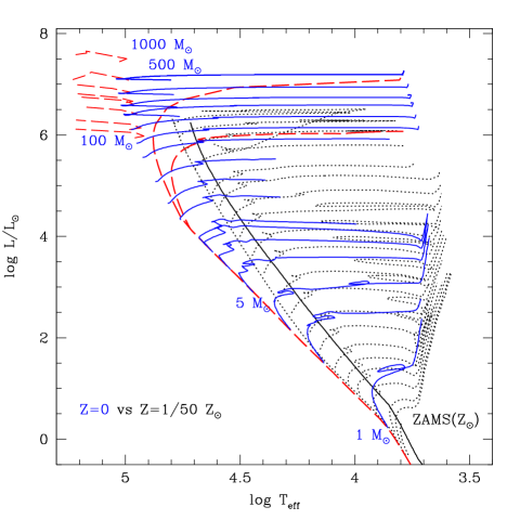
Figure 1: HR–diagram for metal free ($Z=0$, solid and long-dashed lines) and low metallicity ($Z=1/50Z_{\odot}$, dotted) stars. Isochrones of 2 and 4 Myr for $Z=0$ tracks without mass loss are also plotted (long-dashed). The short dashed high mass tracks evolving blueward of the ZAMS are computed assuming strong mass loss. The position of the ZAMS at solar metallicity (Schaller et al. 1992) is shown by the solid line. Pop III tracks and isochrones from Marigo et al. (2001, no mass loss) and Klapp (1983), and El Eid et al. (1983, strong mass loss). $Z=0.0004$ tracks for 0.8 to 150 M_⊙ from Lejeune & Schaerer (2001). Note the important shift of the ZAMS to high $T_{\mathrm{eff}}$ from low metallicity to $Z=0$, as well as the rapid redward evolution of the massive stars

2.2 Stellar tracks

To explore two extreme evolutionary scenarios for massive stars we have constructed two different sets of zero metallicity stellar evolution tracks: 1) no mass loss, 2) strong mass loss (see Fig. 1).

For tracks with no or negligible mass loss (1) we use recent tracks from 1 to 500 M_⊙ calculated with the Geneva stellar evolution code (Feijóo 1999, Desjacques 2000). These tracks, including only the core H-burning phase and assuming small mass loss, have been compared with the tracks of Marigo et al. (2001) up to 100 M_⊙ and additional models up to 500 M_⊙ by Marigo (2000, private communication). Good agreement is found regarding the zero age main sequences (ZAMS), H-burning lifetimes, and the overall appearance of the tracks. The differences due to mass loss in the Geneva models are minor for the purpose of the present work. Furthermore, as the He-burning lifetime is $\la$ 10 % of the main sequence phase and is spent at cooler temperatures (cf. Marigo et al. 2001), neglecting this phase has no consequences for our predictions. This has also been verified by comparisons of integrated stellar populations adopting alternatively the isochrones provided by Marigo et al. (2001).

The “strong mass loss” set (2) consists of a combination of the following stellar tracks for the mass range from 80 to 1000 M_⊙. Tracks of Klapp (1983) for initial masses of 1000 and 500 M_⊙ computed with values of $N=50$ and 100 respectively for the mass loss parameter. For 300, 220, 200, 150, 100, and 80 M_⊙ we adopt the tracks of El Eid et al. (1983). The remaining models (1 to 60 M_⊙) are from the “no mass loss” set. The main difference between the “strong” and “no mass loss” sets is the rapid blueward evolution of the stars in the former case, due to strong increase of the He abundance on the surface of these stars leading to a hot WR-like phase (see Fig. 1). While the use of updated input physics (e.g. nuclear reaction rates) could lead to somewhat different results if recomputed with more modern codes, the predicted tracks depend essentially only on the adopted mass loss (see also Chiosi & Maeder 1986), and remain thus completely valid.

In Figure 1 the two set of tracks are compared to the low metallicity ($Z=1/50$ Z_⊙, dotted lines) models of Lejeune & Schaerer (2000) and the position of a solar metallicity ZAMS (Schaller et al. 1992). This illustrates the well known fact that – due to the lack of CNO elements – the ZAMS of massive Pop III stars is much hotter that their solar or low metallicity counterparts (cf. Ezer & Cameron 1971, El Eid et al. 1983, Tumlison & Shull 2000). In particular this implies that at $Z=0$ stars with $M\ga$ 5 M_⊙ have unusually high temperatures and in turn non-negligible ionising fluxes (cf. Sect. 3) corresponding to normal O-type stars ($T_{\mathrm{eff}}$ $\ga$ 30 kK).

2.3 Evolutionary synthesis models

To calculate the properties of integrated zero metallicity stellar populations we have included the stellar atmosphere models and evolutionary tracks in the evolutionary synthesis code of Schaerer & Vacca (1998). The following changes have been made to adapt the calculations to metal-free populations.

2.3.1 Nebular emission

The potentially strongest H and He recombination lines in the rest-frame UV from Lyman-$\alpha$ longward to H$\alpha$ in the optical spectrum are calculated, namely Lyman-$\alpha$, He ii $\lambda$1640, He ii $\lambda$3203, He i $\lambda$4026, He i $\lambda$4471, He ii $\lambda$4686, H$\beta$, He i $\lambda$5016, He i $\lambda$5876, and H$\alpha$. We assume Case B recombination for an electron temperature of $T_{e}=30000$ K appropriate of metal-free gas and a low electron density ($n_{e}=100$ cm^-3). The emissivities and recombination coefficients of Storey & Hummer (1995) are used in general. For He i $\lambda$4471 we take the data from Osterbrock (1989) for $T_{e}=20000$ K. Lyman-$\alpha$ emission is computed assuming a fraction of 0.68 of photons converted to Lyman-$\alpha$ (Spitzer 1978). For these assumptions the line luminosities (in units of erg s^-1) are thus expressed as

$$L_{l}\,\,[{\rm erg\,s^{-1}}]=c_{l}\,\,(1-f_{\rm esc})\,\,Q_{i}\,\,\,[{\rm s^{-1}}],$$ (1)

where $c_{l}$ are the coefficients given in Table 1, $f_{\rm esc}$ is the photon escape fraction out of the idealised region considered here (we assume $f_{\rm esc}=0$ in our calculations, cf. Sect. 4), and $Q_{i}$ is the ionising photon flux (in units of s^-1) corresponding to the appropriate recombination line. The line emissivities depend only relatively weakly on the assumed conditions. Adopting, e.g. a temperature of $T_{e}=10000$ K leads to an increase of the He ii line luminosities by $\sim$ 10 – 30 %, whereas changes of $\la$ 10 % are found for the H lines ($c_{\rm 1640}=6.40\times 10{-12}$, $c_{{\rm H}\alpha}=1.37\times 10^{-12}$). This lower value of $T_{e}$ is adopted for calculations at non-zero metallicities as in Schaerer & Vacca (1998)

Table 1: Line emission coefficients $c_{l}$ for Case B, $T_{e}=30000$ K, $n_{e}=100$ cm^-3

Line	$c_{l}$ [erg]	appropriate ionising flux $Q_{i}$
Lyman-$\alpha$	$1.04\times 10^{-11}$	$Q({\rm H})$
He ii $\lambda$1640	$5.67\times 10^{-12}$	$Q({\rm He^{+}})$
He ii $\lambda$3203	$3.32\times 10^{-13}$	$Q({\rm He^{+}})$
He i $\lambda$4026	$9.25\times 10^{-13}$	$Q({\rm He^{0}})$
He i $\lambda$4471	$1.90\times 10^{-13}$	$Q({\rm He^{0}})$
He ii $\lambda$4686	$7.13\times 10^{-13}$	$Q({\rm He^{+}})$
H$\beta$	$4.47\times 10^{-13}$	$Q({\rm H})$
He i $\lambda$5016	$1.31\times 10^{-13}$	$Q({\rm He^{0}})$
He i $\lambda$5876	$4.90\times 10^{-13}$	$Q({\rm He^{0}})$
H$\alpha$	$1.21\times 10^{-12}$	$Q({\rm H})$

As we will be studying objects with strong ionising fluxes, nebular continuous emission must also be included. The monochromatic luminosity of the gas is given by

$$L_{\lambda}=\frac{c}{\lambda^{2}}\frac{\gamma_{\rm total}}{\alpha_{B}}(1-f_{\rm esc})Q({\rm H})$$ (2)

(e.g. Osterbrock 1989), where $\alpha_{B}$ is the case B recombination coefficient for hydrogen. The continuous emission coefficient $\gamma_{\rm total}$, including free-free and free-bound emission by H, neutral He and singly ionised He, as well as the two-photon continuum of hydrogen is given by

$$\gamma_{\rm total}=\gamma_{\rm HI}+\gamma_{\rm 2q}+\gamma_{\rm HeI}\frac{n({\rm He}^{+})}{n({\rm H}^{+})}+\gamma_{\rm HeII}\frac{n({\rm He}^{++})}{n({\rm H}^{+})}.$$ (3)

The emission coefficients $\gamma_{i}$ (in units of erg cm³ s^-1 Hz^-1) are taken from the tables of Aller (1984) and Ferland (1980) for wavelength below/above 1 $\mu$m respectively for an electron temperature of 20000 K . The primordial H/He abundance ratio of Izotov & Thuan (1998) is adopted. As a non-negligible He ii ionising flux is obtained in the calculations under certain conditions (cf. below), we also allow for possible continuous emission from the region with doubly ionised He. The relative contribution of the He⁺⁺ and the He⁺ regions is to first order easily calculated from the relative size of the respective Stroemgren spheres and is given by $(n({\rm He}^{++})/n({\rm H}^{+}))/(n({\rm He}^{+})/n({\rm H}^{+}))\sim 2.\times Q({\rm He^{+}})/Q({\rm H})$. As expected, the resulting contribution from the He⁺ region is small, even in the case of the hardest spectra considered here. However, as shown later, the total nebular continuous emission is not negligible for Population III objects even in the rest-UV range.

2.3.2 Initial mass function

The question of the masses and mass distribution of metal-free stars has been studied since the 1960’s (see the volume of Weiss et al. 2000 for recent results).

While the outcome from various hydrodynamical models and other studies still differ, there seems to be an overall consensus that stars with unusually large masses (up to $\sim$ 10³ M_⊙) may form, possibly even preferentially (e.g. Abel et al. 1998, Bromm et al. 1999, 2001, Nakamura & Umemura 2001). Uehara et al. (1996) and Nakamura & Umemura (1999, 2001) also find that the formation of stars with masses down to $\sim$ 1 M_⊙ is not excluded (cf. also Abel et al. 2001). The differences may be of various origins (adopted numerical scheme and resolution, treatment of radiation transfer and optically thick regions etc.).

In view of our ignorance on this issue we adopt a variety of different upper and lower mass limits of the IMF assumed to be a powerlaw, with the aim of assessing their impact on the properties of integrated stellar populations. The main cases modeled here are summarised below in Table 2. Except if mentioned otherwise, the IMF slope is taken as the Salpeter value ($\alpha=$ 2.35) between the lower and upper mass cut-off values M_low and M_up respectively. The consideration of stars even more massive than 1000 M_⊙ (or no mass loss models with $>$ 500 M_⊙) is limited by the availability of evolutionary tracks for such objects. The tabular data given below allows the calculation of integrated populations with arbitrary IMFs for ZAMS populations and the case of a constant SFR .

Table 2: Summary of main model input parameters. All models assume a Salpeter slope for the IMF

Model ID	tracks	Mlow	Mup	symbol in Figs. 6, 7, 8
A	No mass loss	1	100	dotted
B	No mass loss	1	500	solid
C	No mass loss	50	500	long dashed
D	Strong mass loss	1	500	dash – dotted
E	Strong mass loss	50	1000	long dash – dotted
Solar metallicity tracks:
ZS	High mass loss	1	100
$Z=1/50$ Z⊙ tracks:
ZL	Mass loss	1	150

3 Properties of individual stars

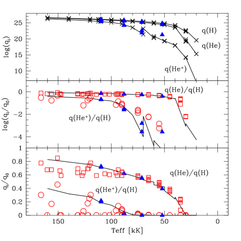
Figure 2: Ionising photon flux (top panel) and hardness of the ionising spectrum (middle and bottom panel) as a function of effective temperature for various atmosphere models. Solid lines connect plane parallel TLUSTY Pop III composition models of various $T_{\mathrm{eff}}$ and $\log g$. Triangles show calculations from the spherically expanding CMFGEN models for Pop III stars. For comparison the pure H and He WR models of Schmutz et al. (1992) are also shown (open squares and circles). Discussion in text

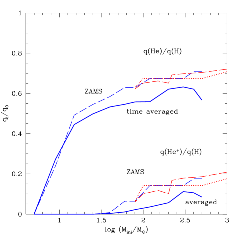
Figure 3: Hardness of the ionising spectrum expressed by $q({\rm He^{0}})/q({\rm H})$ and $q({\rm He^{+}})/q({\rm H})$ as a function of the initial stellar mass. Dashed lines show the hardness of all ZAMS models. The thick lines (dashed: no mass loss, dotted: high mass loss tracks) show the average spectral hardness when stellar evolution effects are taken into account. Note in particular the importance of stellar evolution leading to a decrease of the hardness of the He ii ionising spectrum by approximately a factor of 2

Table 3: Properties of Pop III ZAMS stars

$M_{\rm ini}$	$\log L/L_{\odot}$	$\log T_{\rm eff}$	$Q({\rm H})$	$Q({\rm He^{0}})$	$Q({\rm He^{+}})$	$Q({\rm LW})$	$Q({\rm He^{0}})/Q({\rm H})$	$Q({\rm He^{+}})/Q({\rm H})$
1000.	7.444	5.026	1.607E+51	1.137E+51	2.829E+50	1.727E+51	0.708E+00	0.176E+00
500.	7.106	5.029	7.380E+50	5.223E+50	1.299E+50	7.933E+50	0.708E+00	0.176E+00
400.	6.984	5.028	5.573E+50	3.944E+50	9.808E+49	5.990E+50	0.708E+00	0.176E+00
300.	6.819	5.007	4.029E+50	2.717E+50	5.740E+49	4.373E+50	0.674E+00	0.142E+00
200.	6.574	4.999	2.292E+50	1.546E+50	3.265E+49	2.487E+50	0.674E+00	0.142E+00
120.	6.243	4.981	1.069E+50	7.213E+49	1.524E+49	1.161E+50	0.674E+00	0.142E+00
80.	5.947	4.970	5.938E+49	3.737E+49	3.826E+48	6.565E+49	0.629E+00	0.644E-01
60.	5.715	4.943	3.481E+49	2.190E+49	2.243E+48	3.848E+49	0.629E+00	0.644E-01
40.	5.420	4.900	1.873E+49	1.093E+49	1.442E+47	2.123E+49	0.584E+00	0.770E-02
25.	4.890	4.850	5.446E+48	2.966E+48	5.063E+44	6.419E+48	0.545E+00	0.930E-04
15.	4.324	4.759	1.398E+48	6.878E+47	2.037E+43	1.760E+48	0.492E+00	0.146E-04
9.	3.709	4.622	1.794E+47	4.303E+46	1.301E+41	3.785E+47	0.240E+00	0.725E-06
5.	2.870	4.440	1.097E+45	8.629E+41	7.605E+36	3.760E+46	0.787E-03	0.693E-08

Table 4: Time averaged properties calculated from Pop III tracks with no mass loss

$M_{\rm ini}$	lifetime	$\bar{Q}({\rm H})$	$\bar{Q}({\rm He^{0}})$	$\bar{Q}({\rm He^{+}})$	$\bar{Q}({\rm H}_{2})$	$\bar{Q}({\rm He^{0}})/\bar{Q}({\rm H})$	$\bar{Q}({\rm He^{+}})/\bar{Q}({\rm H})$
1000.	not available
500.00	1.899E+06	6.802E+50	3.858E+50	5.793E+49	7.811E+50	0.567E+00	0.852E-01
400.00	1.974E+06	5.247E+50	3.260E+50	5.567E+49	5.865E+50	0.621E+00	0.106E+00
300.00	2.047E+06	3.754E+50	2.372E+50	4.190E+49	4.182E+50	0.632E+00	0.112E+00
200.00	2.204E+06	2.624E+50	1.628E+50	1.487E+49	2.918E+50	0.621E+00	0.567E-01
120.00	2.521E+06	1.391E+50	7.772E+49	5.009E+48	1.608E+50	0.559E+00	0.360E-01
80.00	3.012E+06	7.730E+49	4.317E+49	1.741E+48	8.889E+49	0.558E+00	0.225E-01
60.00	3.464E+06	4.795E+49	2.617E+49	5.136E+47	5.570E+49	0.546E+00	0.107E-01
40.00	3.864E+06	2.469E+49	1.316E+49	8.798E+46	2.903E+49	0.533E+00	0.356E-02
25.00	6.459E+06	7.583E+48	3.779E+48	3.643E+44	9.387E+48	0.498E+00	0.480E-04
15.00	1.040E+07	1.861E+48	8.289E+47	1.527E+43	2.526E+48	0.445E+00	0.820E-05
9.00	2.022E+07	2.807E+47	7.662E+46	3.550E+41	5.576E+47	0.273E+00	0.126E-05
5.00	6.190E+07	1.848E+45	1.461E+42	1.270E+37	6.281E+46	0.791E-03	0.687E-08

Table 5: Time averaged properties calculated from Pop III tracks with strong mass loss

$M_{\rm ini}$	lifetime	$\bar{Q}({\rm H})$	$\bar{Q}({\rm He^{0}})$	$\bar{Q}({\rm He^{+}})$	$\bar{Q}({\rm H}_{2})$	$\bar{Q}({\rm He^{0}})/\bar{Q}({\rm H})$	$\bar{Q}({\rm He^{+}})/\bar{Q}({\rm H})$
1000.	2.430E+06	1.863E+51	1.342E+51	3.896E+50	2.013E+51	0.721E+00	0.209E+00
500.	2.450E+06	7.719E+50	5.431E+50	1.433E+50	8.345E+50	0.704E+00	0.186E+00
300.	2.152E+06	4.299E+50	3.002E+50	7.679E+49	4.766E+50	0.698E+00	0.179E+00
220.	2.624E+06	2.835E+50	1.961E+50	4.755E+49	3.138E+50	0.692E+00	0.168E+00
200.	2.628E+06	2.745E+50	1.788E+50	2.766E+49	3.028E+50	0.651E+00	0.101E+00
150.	2.947E+06	1.747E+50	1.156E+50	2.066E+49	1.917E+50	0.662E+00	0.118E+00
100.	3.392E+06	9.398E+49	6.118E+49	9.434E+48	1.036E+50	0.651E+00	0.100E+00
80.	3.722E+06	6.673E+49	4.155E+49	4.095E+48	7.466E+49	0.623E+00	0.614E-01

Table 6: Least square fits to the time averaged properties for Pop III stars, metal-poor objects ($Z=1/50$ Z_⊙) and solar metallicity stars for comparison. The time averaged quantities $\log y(M)=a_{0}+a_{1}x+a_{2}x^{2}+a_{3}x^{3}$ (col. 1) are fitted as a function of the initial mass ($x=\log(M/M_{\odot})$) as 2nd or 3rd order polynomials over the mass interval given in col. 2. For masses lower than the range considered the corresponding photon flux $\bar{Q}$ is negligible. $\bar{Q}$ values are in units of photon $s^{-1}$, stellar lifetimes $t_{\star}$ in yr.

Quantity $y$	mass range	$a_{0}$	$a_{1}$	$a_{2}$	$a_{3}$
$Z=0$ tracks with no mass loss:
$\bar{Q}({\rm H})$	9 – 500 M⊙	43.61	4.90	-0.83
$\bar{Q}({\rm H})$	5 – 9 M⊙	39.29	8.55
$\bar{Q}({\rm He^{0}})$	9 – 500 M⊙	42.51	5.69	-1.01
$\bar{Q}({\rm He^{0}})$	5 – 9 M⊙	29.24	18.49
$\bar{Q}({\rm He^{+}})$	5 – 500 M⊙	26.71	18.14	-3.58
$\bar{Q}({\rm H}_{2})$	5 – 500 M⊙	44.03	4.59	-0.77
$t_{\star}$	5 – 500 M⊙	9.785	-3.759	1.413	-0.186
$Z=0$ tracks with strong mass loss:
$\bar{Q}({\rm H})$	80 – 1000 M⊙	46.21	2.29	-0.20
$\bar{Q}({\rm He^{0}})$	80 – 1000 M⊙	45.71	2.51	-0.24
$\bar{Q}({\rm He^{+}})$	80 – 1000 M⊙	41.73	4.86	-0.64
$\bar{Q}({\rm H}_{2})$	80 – 1000 M⊙	46.25	2.30	-0.21
$t_{\star}$	80 – 1000 M⊙	8.795	-1.797	0.332
Solar metallicity tracks:
$\bar{Q}({\rm H})$	7 – 120 M⊙	27.89	27.75	-11.87	1.73
$\bar{Q}({\rm He^{0}})$	7 – 120 M⊙	1.31	64.60	-28.85	4.38
$\bar{Q}({\rm H}_{2})$	15 – 120 M⊙	41.90	7.10	-1.57
$t_{\star}$	7 – 120 M⊙	9.986	-3.497	0.894
$Z=1/50$ Z⊙ tracks:
$\bar{Q}({\rm H})$	7 – 150 M⊙	27.80	30.68	-14.80	2.50
$\bar{Q}({\rm He^{0}})$	20 – 150 M⊙	16.05	48.87	-24.70	4.29
$\bar{Q}({\rm He^{+}})$	20 – 150 M⊙	34.65	8.99	-1.40
$\bar{Q}({\rm H}_{2})$	12 – 150 M⊙	43.06	5.67	-1.08
$t_{\star}$	7 – 150 M⊙	9.59	-2.79	0.63

We now discuss the properties of the ionising spectra and their dependence on assumptions of model atmospheres. The ZAMS properties of individual stars as well as their average properties taken over their lifetime (i.e. including the effect of stellar evolution) are presented next.

3.1 Ionising and H₂ dissociating spectra

The ionising photon fluxes $q_{i}$ and the hardness of the spectrum (described by $q({\rm He^{0}})/q({\rm H})$ and $q({\rm He^{+}})/q({\rm H})$) predicted by various atmosphere models as a function of $T_{\mathrm{eff}}$ are shown in Fig. 2. The ionising photon flux per surface area $q_{i}$, given in units of photons s^-1 cm^-2, is related to the stellar ionising photon flux $Q_{i}$ (in photons s^-1) used later by

$$Q_{i}=4\pi R_{\star}^{2}q_{i}=4\pi R_{\star}^{2}\int_{\nu_{i}}^{\infty}\frac{F_{\nu}}{h\nu}d\nu,$$ (4)

where $R_{\star}$ is the stellar radius, $F_{\nu}$ the spectral flux distribution (in erg cm^-2 s^-1 Hz^-1), and $\nu_{i}$ the frequency of the appropriate ionisation potential. The photon flux $Q({\rm LW})$ in the Lyman-Werner band (11.2 to 13.6 eV) capable to dissociate H₂ is also calculated.

The solid lines in Fig. 2 give the predictions obtained from the plane parallel non-LTE TLUSTY models. As already discussed by Tumlinson & Shull (2000, TS00), this shows in particular the high fraction of photons emitted with energies capable to ionise He i and He ii for stars with $T_{\mathrm{eff}}$ $\ga$ 40 kK and $\ga$ 80 kK respectively.

As the stellar tracks with strong mass loss evolve from the ZAMS (at $\sim$ 100 kK for $M\ga 100M_{\odot}$) blueward, we have also extended the temperature range to the hottest temperatures for which atmosphere models with winds are available (Schmutz et al. 1992, shown as open symbols in Fig. 2). As best shown in the bottom panel, the ratios $q({\rm He^{0}})/q({\rm H})$ and $q({\rm He^{+}})/q({\rm H})$ continue to increase with $T_{\mathrm{eff}}$, as the maximum of the flux distribution has not yet shifted above 54 eV. However, it is important to remember that in the case of atmospheres with winds, the ionising flux also depends on the wind density as illustrated by the dispersion of the Schmutz et al. models for given $T_{\mathrm{eff}}$. For example, for sufficiently dense winds the He ii ionising flux can be completed suppressed (cf. Schmutz et al. 1992). However, for the wind densities obtained in the present models, this situation is not encountered (cf. below).

The ionising properties of ZAMS models for masses between 5 and 1000 M_⊙ are given in Table 3.

The following differences are obtained between various atmosphere models for $T_{\mathrm{eff}}$ between 50 and 100 kK. The plane parallel TLUSTY models show some variation of $q({\rm He^{+}})$ at 70 kK with gravity, with low $\log g$ leading to higher $q({\rm He^{+}})$. As expected, for very hot stars the CMFGEN photosphere-wind models (filled triangles in Fig. 2) show little deviation from the plane parallel models, since the He ii continuum is formed in progressively deeper layers of the atmosphere (e.g. Husfeld et al. 1984, Clegg & Middlemass 1987). The two models at $T_{\mathrm{eff}}$ $\sim$ 70 kK (corresponding to a ZAMS mass of 25 M_⊙) show an increase of $q({\rm He^{+}})$ of up to $\sim$ 1 dex with respect to the TLUSTY model of same $\log g$, due to a depopulation of the He ii groundstate induced by the stellar wind (Gabler et al. 1989). Towards lower $T_{\mathrm{eff}}$ differences between static and spherically expanding atmospheres becomes progressively more important for $q({\rm He^{+}})$. However, in the integrated populations considered later, the emission of He ii ionising photons will be dominated by the hottest objects. We are therefore likely left with the situations where either possible wind effects have no significant impact on the total $q({\rm He^{+}})/q({\rm H})$ hardness, or $q({\rm He^{+}})/q({\rm H})$ is too small to have observable consequences. In conclusion, it appears safe to rely only on non-LTE plane parallel atmospheres to properly describe the ionising fluxes of metal-free stellar populations.

Can other effects, not included in the present model atmosphere grids, affect the ionising spectra ? The effect of non-coherent electron scattering could be important for $T_{\mathrm{eff}}$ $\ga$ 40 kK (Rybicki & Hummer 1994). Test calculations with the CMFGEN code of Hillier & Miller (1998) for some of the above CMFGEN models indicate negligible changes on the ionising photon fluxes. Compton scattering, instead of the commonly implemented Thomson scattering, should not affect the ionising fluxes of normal Pop III stars, as differences appear only above $T_{\mathrm{eff}}$ $\ga$ 150 kK (Hubeny et al. 2001). X-rays, originating from stellar wind instabilities or interactions with magnetic fields, can potentially increase the high energy (He⁺) ionising flux in stars with weak winds (MacFarlane et al. 1994). For Pop III stars such a hypothesis remains highly speculative. The adopted model atmospheres should thus well describe the spectra of the objects considered here.

3.1.1 Comparisons with other Pop III calculations

As expected, our calculations for individual stars of a given $T_{\mathrm{eff}}$ agree quite well with those of TS00 based also on the TLUSTY model atmospheres. As briefly mentioned above, small differences are found with their ZAMS positions calculated with simplified stellar models. For integrated populations the use of a proper ZAMS leads to somewhat softer spectra (cf. Sect. 4.1).

As pointed out by Bromm et al. (2001) the spectral properties of stars with $M\ga$ 300 M_⊙ are essentially independent of stellar mass, when normalised to unit stellar mass. The degree to which this holds can be verified from Table 3. If correct, it would imply that the total spectrum of such a population would be independent of the IMF and only depend on its total mass. Our results for the 1000 M_⊙ ZAMS star are in rather good agreement with the ionising fluxes of Bromm et al. (2001, their Table 1) . However, as already apparent from their Fig. 3 the deviations from this approximate behaviour are not negligible for the He⁺ ionising flux. In consequence we find e.g. $Q({\rm H})$ reduced by 12 % and He ii recombination line strengths reduced by a factor 2 for a population with a Salpeter IMF from 300 to 1000 M_⊙! Larger difference are obviously obtained for IMFs with M_low $<$ 300 M_⊙. Further differences (due to the inclusion of nebular continuous emission) with Bromm et al. (2001) are discussed in Sect. 4.

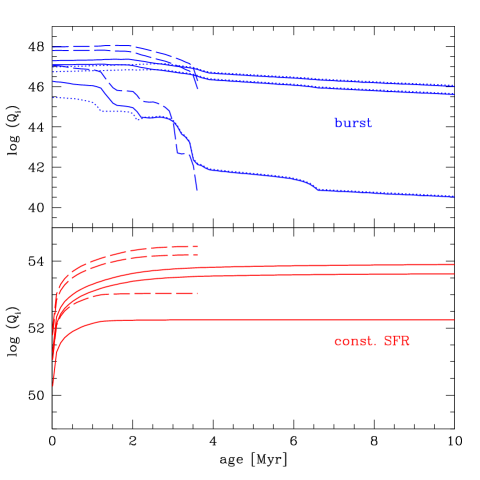
Figure 4: Ionising photon fluxes $Q({\rm H})$, $Q({\rm He^{0}})$ and $Q({\rm He^{+}})$ as a function of time for instantaneous burst models (upper panel) or constant star formation (lower panel). For each group of 3 lines (using the same symbols) $Q({\rm H})$, $Q({\rm He^{0}})$ and $Q({\rm He^{+}})$ are given from top to bottom. Different IMFs are illustrated by the dotted (model ID A), solid (model B) and long-dashed lines (model C) respectively (cf. Table 2). The units are photon s^-1 M_⊙^-1 for the burst and photon s^-1 normalised per unit SFR (in M_⊙ yr^-1) for constant SF. Note in particular the rapid decrease of the He ii ionising flux $\sim$ 3–4 Myr after the burst

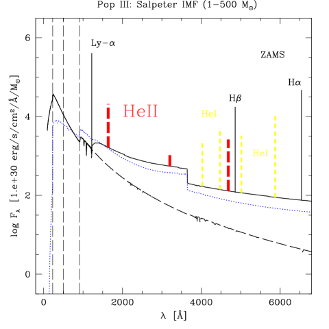
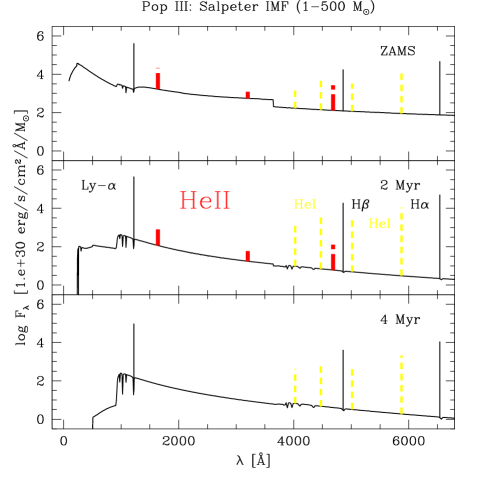
Figure 5: Spectral energy distribution (SED) including H and He recombination lines for model B (solid line, see Table 1 for line identifications). Left panel: ZAMS population. The pure stellar continuum (neglecting nebular emission) is shown by the dashed line. For comparison the SED of the $Z=1/50Z_{\odot}$ population (model ZL: Salpeter IMF from 1 – 150 M_⊙) is shown by the dotted line. The vertical dashed lines indicate the ionisation potentials of H, He⁰, and He⁺. Note the presence of the unique He ii features (shown as thick dashed lines) and the importance of nebular continuous emission. Right panel: temporal evolution of the spectrum for 0, 2 and 4 Myr showing the rapid change of the emission line spectrum, characterised by the disappearance of the He ii lines

3.2 Time averaged ionising properties

As clear from Fig. 1, massive stars evolve rapidly toward cooler temperatures during their (short) lifetime in the absence of strong mass loss. It is thus evident that especially the He ii ionising flux will strongly decrease with age. To quantify this effect we have calculated the lifetime averaged ionising flux $\bar{Q}_{i}$ along the evolutionary tracks, defined by

$$\bar{Q}_{i}(M)=\frac{\int_{0}^{t_{\star}(M)}Q_{i}(t,M)dt}{t_{\star}(M)},$$ (5)

where $t_{\star}$ is the stellar lifetime. The results calculated for both sets of tracks (no mass loss, strong mass loss) are given in Tables 4 and 5 respectively. For convenience we also provide simple fits (linear or quadratic) of these values as a function of the initial mass $M$ in Table 6. Together with $t_{\star}$ the average ionising flux $\bar{Q}_{i}$ defined in this manner in particular allows one to calculate the correct values of the ionising flux, recombination line luminosities etc. for integrated populations at equilibrium, i.e. for the asymptotic value obtained for a constant star formation rate.

The time averaged hardness as a function of mass is compared to the ZAMS value in Fig. 3. For tracks without mass loss, $\bar{Q}({\rm He^{+}})/\bar{Q}({\rm H})$ is found to be a factor of two or more below the ZAMS value. Smaller differences are obtained for obvious reasons for $\bar{Q}({\rm He^{0}})/\bar{Q}({\rm H})$. Only in the case of very strong mass loss, the equilibrium value of the hardness of the ionising spectrum is found to be essentially identical as the ZAMS value.

For Pop I stars the effect of time dependent and time averaged ionising fluxes and the spectral hardness based on recent atmosphere models have been studied earlier in various contexts (analysis of O star populations from integrated spectra, studies of the diffuse ionised gas; see e.g. Schaerer 1996, 1998). For comparison sake the resulting fits for solar metallicity and 1/50 Z_⊙ are also given in Table 6.

4 Population III “galaxies”

4.1 Time evolution of integrated spectra

The temporal evolution of the integrated ionising photon flux of an instantaneous burst and the case of constant star formation is plotted in Fig. 4 for different IMFs. Most notable is the rapid decrease of the He ii ionising flux in a burst, due to the evolution of the most massive stars off the hot ZAMS and due to their short lifetime.

Our values compare as follows with other calculations of $Q({\rm H})$ available in the literature: when scaled to the same lower mass cut-off of the IMF ($M_{\rm low}=0.024$ M_⊙), our ZAMS model for IMF A (Table 2) agrees with $Q({\rm H})$ (age $\sim$ 0) of Cojazzi et al. (2000). The same holds for $Q({\rm H})$ of Ciardi et al. (2000), when adopting their IMF (Salpeter from 1 to 40 M_⊙). A good agreement is found with $Q({\rm H})$ of TS00 (ZAMS population with a Salpeter IMF from 0.1 to 100 M_⊙), whereas the slightly cooler ZAMS (cf. Sect. 3.1.1) implies a somewhat softer spectrum ($Q({\rm He^{+}})$/$Q({\rm H})$ $\sim$ 0.03 instead of 0.05). Differences with Bromm et al. (2001) have already been discussed above (Sect. 3.1.1).

Spectral energy distributions of integrated zero metallicity stellar populations are shown in Fig. 5 for the case of a Salpeter IMF from 1 to 500 M_⊙ and instantaneous bursts of ages 0 (ZAMS), 2, and 4 Myr. Overplotted on the continuum (including stellar $+$ nebular emission: solid lines) are the strongest emission lines for illustration purpose. In the left panel we show for comparison the spectrum of a burst at low metallicity (1/50 Z_⊙, Salpeter IMF from 1 – 150 M_⊙; dotted line). The striking differences, most importantly in the ionising flux above the He ii edge ($>$ 54 eV), have already been discussed by TS00. The comparison of the total spectrum (solid line) with the pure stellar emission (dashed) illustrates the importance of nebular continuous emission neglected in earlier studies (TS00, Bromm et al. 2001), which dominates the ZAMS spectrum at $\lambda\ga$ 1400 Å. The nebular contribution, whose emission is proportional to $Q({\rm H})$ (Eq. 2), depends rather strongly on the age, IMF, and star formation history. For the parameter space explored here (cf. Table 2), we find that nebular continuous emission is not negligible for bursts with ages $\la$ 2 Myr and for constant star formation models.

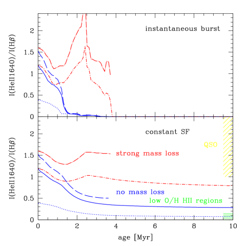
Figure 6: Temporal evolution of the relative He ii $\lambda$1640/H$\beta$ line intensity for various models. Upper panel: instantanous burst models with different IMFs and for no mass loss tracks (dotted, dashed, solid) and high mass loss (dash-dotted, long dash – dotted; see symbols in Table 2). Lower panel: same as above for constant star formation models. The shaded ranges on the right indicate He ii $\lambda$1640/H$\beta$ intensities of quasars and maximum values expected for metal-poor H ii regions. For the IMFs considered here $I(1640)/I({\rm H}\beta)$ can reach the high values typical of quasars for very young bursts or in the (extreme) case of high mass loss.

The spectra in Fig. 5 show in addition to the H and He i recombination lines the presence of the strong He ii $\lambda\lambda$ 1640, 3203, and 4686 recombination lines, which — due to the exceptional hardness of the ionising spectrum — represent a unique feature of Pop III starbursts compared to metal enriched populations (cf. TGS01, Oh et al. 2001a, Bromm et al. 2001). Another effect highlighted by this Figure is the rapid temporal evolution of the recombination line spectrum. Indeed, already $\ga$ 3 Myr after the burst, the high excitation lines are absent, for the reasons discussed before. In the case of constant star formation, the emission line spectrum at equilibrium is similar to a burst of $\sim$ 1.3 Myr (cf. Fig. 6).

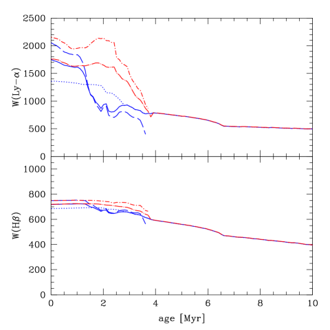
Figure 7: Temporal evolution of Lyman-$\alpha$ (top) and H$\beta$ (bottom) for instantaneous burst models. Note that very large maximum equivalent widths are obtained. As the IMF and track variations considered here concern only the most massive stars ($M\ga$ 50 – 100 M_⊙) the predictions are only affected at young ages ($\la$ 4 Myr)

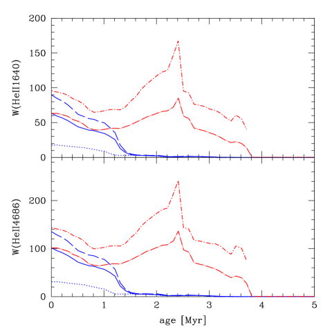
Figure 8: Same as 7 for the He ii $\lambda$1640 (top) and He ii $\lambda$4686 (bottom) recombination lines. Note that large maximum equivalent widths.

Figure 6 shows the temporal evolution of the line intensity of He ii $\lambda$1640 with respect to H$\beta$ for different IMFs, instantaneous bursts (upper panel) or constant star formation (lower panel), and the two sets of stellar tracks (see model designations in Table 2). As the lifetime of the stars affected by the IMF variations considered here is $\sim$ 2 – 4 Myr, no changes are seen at ages $\ga$ 4 Myr. The following points are worthwhile noticing:

• already for a “normal” IMF with M_up = 100 M_⊙ the maximum He ii $\lambda$1640 intensity is exceptionally large for pure stellar photoionisation compared to metal-poor stellar populations (cf. TS00);

• extending the IMF up to 500 – 1000 M_⊙ leads to $I(1640)/I({\rm H}\beta)$ up to $\sim$ 1.5 – 2;

• in the unlikely case of high mass loss the He ii $\lambda$1640 intensity is maintained for up to $\sim$ 4 Myr;

• for models without mass loss, the equilibrium values of $I(1640)/I({\rm H}\beta)$ are of the order of $\sim$ 0.1 – 0.6 for the IMF range considered here. For comparison, $I(1640)/I({\rm H}\beta)\sim$ 1.0 – 3.2 for a power law spectrum $L_{\nu}\propto\nu^{-\alpha}$ and typical values $\alpha\sim$ 1 – 1.8 for quasars (Elvis et al. 1994, Zheng et al. 1997), and the largest intensities in (rare) metal-poor H ii regions are $I(1640)/I({\rm H}\beta)\la$ 0.15, as expected from their measured He ii $\lambda$4686 intensity.

The equivalent widths for the strongest H and He ii lines and their dependence on the IMF and stellar tracks are shown in Figs. 7 and 8. Maximum equivalent widths of $\sim$ 700 and 3200 Å are predicted for the optical lines of H$\beta$ and H$\alpha$ (not shown) respectively. W(Lyman-$\alpha$) reaches values up to $\sim$ 2100 Å at the ZAMS, but is potentially affected or destroyed by radiation transfer or other effects (cf. Tenorio-Tagle et al. 1999). The maximum equivalent width of the He ii $\lambda\lambda$ 1640 and 4686 recombination lines on the ZAMS is predicted to be $\sim$ 100 and 150 Å respectively.

What variations are typically obtained for different IMF slopes ? Varying $\alpha$ between 1. and 3. one finds the following changes for bursts at age 0 Myr with respect to the Salpeter slope: for models A and B $I(1640)/I({\rm H}\beta)$ (and the other He ii intensities) varies between $\sim$ – 60 % and + 50 %, $W({\rm Ly-}\alpha)$ changes by not more than $\sim$ 20 %, and $W($He ii $\lambda$1640$)$ varies between $\sim$ – 50 % and + 60 %. For obvious reasons, populations most biased towards massive stars (i.e. large values of M_low) are the least sensitive to the exact IMF slope (cf. Bromm et al. 2001). E.g., the above quantities vary by $\la$ 20 % for model C.

Much larger Lyman-$\alpha$ and He ii $\lambda$1640 equivalent widths ($\sim$ 3100 and 1100 Å respectively) have been predicted for a ZAMS population of exclusively massive stars by Bromm et al. (2001). This overestimate is due to two effects acting in the same direction: their simplified use of the spectrum of a 1000 M_⊙ star with the hardest spectrum as representative for the entire population, and most importantly the neglect of nebular continuous emission, which — for the case of a Salpeter IMF from 300 to 1000 M_⊙ — contributes $\sim$ 75 % of the total light at $\lambda$ 1640 and thus strongly reduces the He ii $\lambda$1640 equivalent width (cf. above). Accounting for these effects yields W(Lyman-$\alpha$) $\sim$ 2000 and W(1640) $\sim$ 120 Å for their IMF.

Our calculation of the nebular continuous emission assumes density bounded objects, i.e. negligible escape of Lyman continuum photons out of the “Pop III galaxies” ($f_{\rm esc}\ll 1$). If this is not the case, one likely has a situation where nevertheless all He ii ionising photons are absorbed — i.e. $L($He ii $\lambda$1640$)$ remains identical — while some H ionising photons escape thereby reducing the continuum emission (proportional to $Q({\rm H})$ (Eq. 2). Although the escape fraction of ionising photons in distant galaxies or the first building blocks thereof remains badly known, there are theoretical and observational indications for rather low escape fractions, of the order of $\sim$ 10 % (see e.g. Leitherer et al. 1995, Dove et al. 2000, Steidel et al. 2001, Hui et al.2001). For such moderate an escape fraction, nebular continuous emission remains thus dominant when strong emission lines are expected, leading to He ii equivalent widths not much larger than predicted here. Estimates for small Pop III halos suggest, however, large escape fractions (Oh et al. 2001b). In short, the caveat regarding the uncertainty on $f_{\rm esc}$, which affects both emission line luminosities and nebular continuum emission, must be kept in mind. A more detailed treatment including geometrical effects, radiation transfer etc. (cf. Ciardi et al. 2001) are beyond the scope of our estimates.

Regarding the equivalent widths, we conclude that in any case the maximum values of $W($Lyman-$\alpha$$)$ and $W($He ii $\lambda$1640$)$ of metal-free populations are $\sim$ 3–4 and $\sim$ 80 times larger than the values predicted for very metal-poor stellar populations ($Z=1/50$ Z_⊙) with a “normal” IMF including stars up $\sim$ 100 M_⊙. When measured in the rest-frame, these will further be amplified by a factor $(1+z)$, where $z$ is the redshift of the source.

4.2 Star formation indicators

In the case of constant star formation, the ionising properties tend rapidly (typically over $\sim$ 5 – 10 Myr depending on the IMF) to their equilibrium value, which is then proportional to the star formation rate (SFR). In particular, recombination line luminosities $L_{l}$ are then simply given by

$$L_{l}=c_{l}\,(1-f_{\rm esc})\,Q_{i}\left(\frac{\rm SFR}{M_{\odot}{\rm yr}^{-1}}\right)=f_{l}\left(\frac{\rm SFR}{M_{\odot}{\rm yr}^{-1}}\right).$$ (6)

The predicted values $f_{l}$ (in erg s^-1) for He ii $\lambda$1640 and H$\alpha$ for the IMFs considered here are given in Table 7 for the case of a negligible escape fraction of ionising photons ($f_{\rm esc}=0$). For other lines, or to compute the $Q_{i}$ not listed explicitly, the corresponding value can easily be derived using Eq. 1 and the emission coefficients in Table 1. Also listed are the He i ionising production and the photon flux in the Lyman Werner band of H₂ for a star formation rate of 1 M_⊙ yr^-1. For comparison with SFR indicators used for “normal” galaxies we also indicate the mass conversion factor $c_{M}$ expressing the relative masses between our model IMF and a “standard” Salpeter IMF with M_low $=$ 0.1 and M_up $=$ 100 M_⊙ used frequently throughout the literature, i.e. $c_{M}=\int_{0.1}^{100}M\Phi(M)dm/\int_{M_{\rm low}}^{M_{\rm up}}M\Phi(M)dm$.

Table 7: Line luminosities, supernova rates, and photon and metal production for constant star formation models normalised to SFR $=$ 1 M_⊙ yr^-1

ID	$c_{M}$	$f_{{\rm H}\alpha}$	$f_{1640}$	$Q({\rm He^{0}})$	$Q({\rm LW})$	$\bar{E_{Q}}$	SNR	$M_{\rm ej}$	$M_{\rm ej}({\rm C})$	$M_{\rm ej}({\rm O})$	$M_{\rm ej}({\rm Si})$	$\eta$
		[erg s-1]		[(ph s-1)/(M⊙ yr-1)]		[eV]	[M⊙-1]	[M⊙/(M⊙ yr-1)]
A	2.55	7.88e+41	1.91e+40	3.15e+53	3.17e+53	26.70	0.019	0.0076	0.0013	0.0030	0.0005	0.065
B	2.30	1.03e+42	9.98e+40	4.34e+53	3.29e+53	27.86	0.016	0.030	0.0023	0.014	0.0045	0.022
C	14.5	3.32e+42	8.38e+41	1.54e+54	4.52e+53	29.69	0.0016	0.14	0.0065	0.067	0.025	0.016
D	2.30	1.14e+42	3.12e+41	5.26e+53	3.36e+53	30.55	0.016
E	12.35	4.10e+42	2.33e+42	2.21e+54	3.65e+53	35.15	0.0013
Solar metallicity tracks:
ZS	2.55	3.16e+41	5.12e+39	5.56e+52	3.60e+53	20.84	0.019	0.038⋆				0.0036⋆
$Z=1/50$ Z⊙ tracks:
ZL	2.47	6.92e+41	1.70e+39	1.55e+53	5.31e+53	21.95	0.019	0.023	0.0025	0.014	0.0014	0.014
⋆ Including stellar wind mass loss, SN Ibc, and SNII

Compared to the “standard” H$\alpha$ SFR indicator for solar metallicity objects (cf. Kennicutt 1998, Schaerer 1999) $L({\rm H}\alpha)$ is $\sim$ 2.4 times larger for a Pop III object with the same IMF, given the increased $Q({\rm H})$ production (cf. TS00 and above). Obviously, for IMFs more weighted towards high mass stars, the SFR derived from H$\alpha$ (or other H recombination lines) is even more reduced compared to using the standard Pop I SFR indicator. If detected, He ii $\lambda$1640 can also be used as a star formation indicator as already pointed out by TGS01. Their corresponding value is $f_{1640}=8.4\,10^{40}\times f_{\rm evol}$, with $f_{\rm evol}\sim 0.4$ (2.) accounting in an approximate way for stellar evolution effects without (with) mass loss. Including the full sets of evolutionary tracks we find $f_{1640}=1.91\,10^{40}$, for the 1–100 M_⊙ IMF, i.e. less He ii emission than TGS01. Varying the IMF slope $\alpha$ between 1. and 3. leads to changes of $f_{{\rm H}\alpha}$ ($f_{1640}$) by $\sim\pm$ 0.5 (0.9) dex for models A and B, and to minor changes ($\la$ 0.1 dex) for model C. With the fits given in Table 6 the line luminosities can easily be computed for arbitrary IMFs.

In passing we note that the He⁺ ionising flux per unit SFR used by Oh et al. (2001a) to estimate the expected number of sources with detectable He ii recombination lines has been overestimated: for a constant SFR and a Salpeter IMF up to 100 M_⊙ the hardness $Q({\rm He^{+}})$/$Q({\rm H})$ $\sim$ 0.005 is a factor 10 lower than their $Q$ value adopted. However, the Lyman continuum production is increased over the value they adopted, leading thus to a net reduction of their flux $J_{\rm 1640}^{\rm stars}$ by a factor 1.9 (4.8) for a Salpeter IMF with M_low = 1 (0.1) and M_up=100 M_⊙ (cf. Tables 7 and 1). Further issues regarding the photometric properties and the detectability of Pop III sources will be discussed in Pelló & Schaerer (2001).

4.3 Photon and heavy element production

Various other properties related to the photon and heavy element production are given in Table 7 for the case of constant star formation normalised to SFR $=$ 1 M_⊙ yr^-1. Columns 5 and 6 give $Q({\rm He^{0}})$, the He⁰ ionising flux, and the photon flux in the Lyman-Werner bands $Q({\rm LW})$ respectively, both in units of (photon s^-1)/(M_⊙ yr^-1). The average energy $\bar{E_{Q}}$ (in eV) of the Lyman continuum photons is in col. 7.

To estimate the metal production of Pop III objects we have used the SN yields of Woosley & Weaver (1995) for progenitor stars between 8 and 40 M_⊙ and the results of Heger et al. (2000) and Heger & Woosley (2001) for very massive objects of pair creation SN originating from stars in the mass range $\sim$ 130 to 260 M_⊙ (cf. also Ober et al. 1993). As the pair creation SN models of Heger and collaborators are calculated starting with pure helium cores, we have adopted the relation $M_{\alpha}\sim 0.5\,M_{\rm ini}$ from Ober et al. (1983) to calculate the initial mass $M_{\rm ini}$. We neglect the contribution from longer lived intermediate mass stars (1 $\la M/M_{\odot}\la$ 8). Non-rotating stars more massive than $\sim$ 260 M_⊙ are expected to collapse directly to a black hole producing no metals (cf. Rackavy et al. 1967, Bond et al. 1984).

The SN rate SNR including “normal” SN and pair creation SN is given in col. 8 of Table 7 (in units of SN per solar mass of stars formed). The total mass of metals $M_{\rm ej}$ produced including all elements heavier than He is given in col. 9. Columns 10, 11, and 12 indicate the contribution of C, O and Si. The ejected masses are given in units solar mass per unit SFR. Note that the models C and E with a lower mass cut-off M_low $=$ 50 M_⊙ of the IMF represent cases with solely pair creation SN (no SN type II), models A (plus the cases ZS and ZL with non-zero metallicity) include only SNII, and models B and D include both SN types. Finally the dimensionless “conversion efficiency” of ionising photons to rest mass (cf. Madau & Shull 1996)

$$\eta\equiv\frac{\int_{0}^{\infty}\int_{\nu_{H}}^{\infty}L_{\nu}d\nu dt}{M_{\rm ej}\,c^{2}}=\frac{Q({\rm H})*\bar{E_{Q}}}{M_{\rm ej}\,c^{2}},$$ (7)

with the spectral luminosity $L_{\nu}$, is given in col. 13. It is useful to remind that, since both the metal and photon production is dominated by massive stars, $\eta$ is independent of the IMF at masses $M\la$ 5–8 M_⊙, and depends little on the exact shape of the IMF.

The SNR per unit mass depends little on the upper mass cut-off, as most of the mass resides in low mass stars. For cases C and E with M_low = 50 M_⊙ the SNR is reduced, since pair creation SN from stars of a limited mass range ($\sim$ 130 – 260 M_⊙) are the only explosive events.

As evident from the yields of Woosley & Weaver (1995) and shown in Table 7, Population III stars convert – for “standard” IMFs – less of their initial mass into metals than stars of non-zero metallicity. However, for IMFs favouring more strongly massive stars, allowing in particular for pair creation SN ejecting up to half of their initial mass, the metal production per unit stellar mass can be similar to or larger than for solar metallicity.

The photon conversion efficiency of rest mass to ionising continuum, $\eta$, of metal-poor and metal-free populations is increased by factors of $\sim$ 3 - 18 compared to solar metallicity. In great part this is due to increased ionising photon production. The underlying changes of all quantities on which $\eta$ depends are listed in Table 7. The increase of $\eta$ from Z_⊙ to 1/50 Z_⊙ indicates already a substantially larger photon to heavy element production which must have occurred in the early Universe.

In passing we note that our value of $\eta\sim 0.36\%$ (or 0.5 % neglecting stellar mass loss and SNIbc) is larger than the value of 0.2 % given by Madau & Shull (1996), which, given the quoted assumptions appears to be erroneous. This can be easily seen by noting the good agreement between our photon production calculation and other calculations in the literature (e.g. the H$\alpha$ SFR calibration of Kennicutt 1998, Glazebrook et al. 1999). In addition one can easily estimate the metal production from noting that $M_{\rm ej}(M)=fM_{\rm ini}$, with typically $f\sim 0.1$ (Woosley & Weaver 1995) and integrating over the IMF, which confirms our calculations.

Finally the predicted ejecta of carbon, oxygen, and silicon show some interesting variations with the IMF. From the “standard” IMF (A) to an IMF producing exclusively very massive stars (model C), the oxygen/carbon ratio (O/C) $\sim$ 0.8 (O/C)_⊙ increases by a factor $\sim$ 4, while increases from Si/C $\sim$ 1.8 (Si/C)_⊙ by a factor of $\sim$ 10! It is interesting to compare these values with current measurements of abundance ratios in the Lyman-$\alpha$ forest, which indicate an overabundance of Si/C $\sim$ 2 – 3 (Si/C)_⊙ (Songaila & Cowie, 1996, Giroux & Shull 1997), but possibly up to $\sim$ 10 times solar, depending on the adopted ionising UV background radiation field (Savaglio et al. 1997, Giroux & Shull 1997). If the ejecta from Pop III objects are responsible for the bulk of metals in the Lyman-$\alpha$ forest, it would appear that IMFs strongly favouring massive stars seem to be excluded by studies finding a modest Si/C overabundance. The use of more detailed chemical evolution models including also intermediate mass stars (cf. Abia et al. 2001) and additional studies on abundances in the Ly$\alpha$ forest should hopefully provide stronger constraints on early nucleosynthesis and the IMF of Pop III stars.

5 Summary and discussion

The main aim of present study was to construct realistic models for massive Population III stars and stellar populations to study their spectral properties, including their dependence on age, star formation history, and most importantly on the IMF, which remains very uncertain for such objects.

We have calculated extensive sets of non-LTE model atmospheres appropriate for metal-free stars with the TLUSTY code (Hubeny & Lanz 1995) for plane parallel atmospheres. The comparison with non-LTE models including stellar winds, constructed with the comoving frame code CMFGEN of Hillier & Miller (1998), shows that even in the presence of some putative (weak) mass loss, the ionising spectra of Pop III stars differ negligibly from those of plane parallel models, in stark contrast with Pop I stars (Gabler et al. 1989, Schaerer & de Koter 1997). As already discussed by Tumlinson & Shull (2000), the main salient property of Pop III stars is their increased ionising flux, especially in the He⁺ continuum ($>$ 54 eV).

The model atmospheres have been introduced together with recent metal free stellar evolution tracks from the Geneva and Padova groups (Feijóo 1999, Desjacques 2000, Marigo et al. 2000) and older Pop III tracks assuming strong mass loss (Klapp 1983, El Eid et al. 1983) in the evolutionary synthesis code of Schaerer & Vacca (1998) to study the temporal evolution of individual Pop III stars and stellar populations.

The main results obtained for individual Pop III stars are the following (Sect. 3):

• Due to their redward evolution off the zero age main sequence (ZAMS) the spectral hardness measured by the He⁺/H ionising flux is decreased by a factor $\sim$ 2 when averaged over their lifetime. If such stars would suffer strong mass loss, their spectral appearance could, however, remain similar to that of their ZAMS position.

• The ionising photon fluxes of H, He⁰, He⁺, and the flux in the Lyman-Werner band dissociating H₂ have been tabulated and detailed fit formulae are given for stars from 5 to 1000 M_⊙. These can in particular be used to calculate with arbitrary IMFs the properties of ZAMS populations or cases of constant SFR. For comparison the same quantities are also given for solar metallicity and 1/50 Z_⊙.

The integrated spectral properties including line emission from H, He i, He ii recombination lines (treated e.g. by TS00, Bromm et al. 2001) and nebular continuous emission — neglected in all earlier studies — have been calculated for instantaneous bursts and constant formation rates. Various assumptions on the mass cut-offs of the IMF including a “standard” IMF from 1 to 100 M_⊙ or IMFs forming exclusively very massive stars have been considered (see Table 2).

The main results regarding integrated stellar populations are as follows (Sect. 4):

• For young bursts and the case of a constant SFR, nebular continuous emission dominates the spectrum or is at least important to properly predict it redward of Lyman-$\alpha$ if the escape fraction $f_{\rm esc}$ of ionising photons out of the observed region is small or negligible. In consequence predicted emission line equivalent widths are considerably smaller than found in earlier studies, whereas the detection of the continuum is eased. Maximum equivalent widths of W(Ly$\alpha$) $\sim$ 1700 and W(He ii $\lambda$1640) $\sim$ 120 Å are predicted for a Salpeter IMF with M_up $\sim$ 500 – 1000 M_⊙. Nebular line and continuous emission strongly affect the broad band photometric properties of Pop III objects and (see Schaerer & Pelló 2001, Pelló & Schaerer 2001). Detailed treatment models including geometrical effects, radiation transfer etc. (cf. e.g. Ciardi et al. 2001) will be useful to constrain $f_{\rm esc}$ more precisely.

• Due to the redward stellar evolution and short lifetimes of the most massive stars, the hardness of the ionising spectrum decreased rapidly, leading to the disappearance of the characteristic He ii recombination lines after $\sim$ 3 Myr in instantaneous bursts.

• He ii $\lambda$1640, H$\alpha$ (and other) line luminosities usable as indicators of the star formation rate are given for the case of a constant SFR (Table 7)). For obvious reasons such indicators depend strongly on the IMF.

• Accounting for SNII and pair creation supernovae we have also calculated supernova rates, the metal production, and the conversion efficiency of ionising photons to rest mass, $\eta$ (Table 7). For a “standard” IMF with M_up $=$ 100 M_⊙ the increased photon production and the reduced metal yields of Pop III stars lead to an increase of $\eta$ by a factor of 5 to 18 when compared to low (1/50 Z_⊙) or solar metallicity. In the presence of very massive stars ($M\sim$ 130 – 260 M_⊙) leading to pair creation SN, somewhat lower values of $\eta\sim$ 1.6 to 2.2 % are obtained. In any case metal-poor and metal-free populations are much more efficient producers of ionising photons “per baryon” (per unit heavy element rest mass energy) than at solar metallicity, where $\eta\sim$ 0.36 %.

• Finally the ejected masses of C, O, and Si of Pop III objects have been calculated. The O/C abundance and even more so Si/C increase to highly supersolar values if very massive stars leading to pair creation SN form. How far measurements of such abundance ratios, e.g. in the Lyman-$\alpha$ forest, can be used to constrain the IMF of the first stellar objects, remains currently unclear, as also discussed by Abia et al. (2001).

The present model set should also be useful to explore the feasibility of future direct observations of Pop III “galaxies” and to optimise search strategies for such objects. We have started undertaking such studies (Schaerer & Pelló 2001, Pelló & Schaerer 2001).

Tumlinson et al. (2001) speculate that some emission line objects found in deep Lyman-$\alpha$ surveys could actually be He ii $\lambda$1640 emitters such as the metal-free galaxies discussed here. Recently Oh et al. (2001a) have estimated the number of Pop III sources and mini quasars emitting strong He ii lines. Although still speculative, their calculations predict sufficient sources for successful detections with deep, large field observations foreseeable with the Next Generation Space Telescope or future instruments on ground-based 10m class telescopes. Pilot studies now also start to address the question of dust formation and obscuration in the early Universe (Todini & Ferrara 2001), which remain a concern for observations. In any case the upcoming decade should bring a great wealth of new information on the early Universe, and possibly already the first in situ detection of the long sought Population III objects.

- (1) Abia, C., Dominguez, I., Straniero, O., Limongi, M., Chieffi, A., Isern, J., 2001, ApJ, 557, 126
- (2) Abel, T., Anninos, P.A., Norman, M.L., Zhang, Y., 1998, ApJ, 508, 518
- (3) Abel, T., Bryan, G.L., Norman, M.L., 2000, ApJ, 540, 39
- (4) Abel, T., Bryan, G.L., Norman, M.L., 2001, Science, submitted
- (5) Baraffe, I., Heger, A., Woosley, S.E., 2001, ApJ, 552, 464
- (6) Barkana, R., Loeb, A., 2001, Physics Reports, 349, 125 (cf. astro-ph/0010468)
- (7) Bond, J.R., Arnett, W.D., Carr, B.J., 1984, ApJ, 280, 825
- (8) Bromm, V., Coppi, P.S., Larson, R.B., 1999, ApJ, 527, L5
- (9) Bromm, V., Coppi, P.S., Larson, R.B., 2001, ApJ, in press (astro-ph/0102503)
- (10) Bromm, V. , Kudritzki, R.P., Loeb, A., 2001, ApJ, 552, 464
- (11) Cerviño, M., Knödlseder, J., Schaerer, D., von Ballmoos, P., Meynet, G., 2000, A&A, 363, 970
- (12) Chavez, M., et al., 2001, in “The link between Stars and Cosmology”, Eds. Chavez et al., Kluwer, in press
- (13) Chiosi, C., Maeder, A., 1986, ARAA, 24, 329
- (14) Ciardi, B., Ferrara, A., Governato, F., Jenkins, A., 2000, MNRAS, 314, 611
- (15) Ciardi, B., Ferrara, A., Marri, S., Raimondo, G., MNRAS, 2001, 324, 381
- (16) Clegg, R.E.S., Middlemass, D., 1987, MNRAS, 228, 759
- (17) Cojazzi, P., Bressan, A., Lucchin, F., Pantano, O., Chavez, M., 2000, MNRAS, 315, L51
- (18) de Koter, A., Lamers, H.J.G.L.M., Schmutz, W., 1996, A&A, 306, 501
- (19) Desjacques, V., 2000, Diploma thesis, Geneva Observatory
- (20) Dove, J.B., Shull, M.J., Ferrara, A., 2000, ApJ, 531, 846
- (21) El Eid, M.F., Fricke, K.J., Ober, W.W., 1983, A&A, 119, 54
- (22) Elvis, M., et al., 1994, ApJS, 95, 1
- (23) Ezer, D., Cameron, A.G.W., 1971, Ap&SS, 14, 399
- (24) Feijóo, J.M., 1999, Diploma thesis, Geneva Observatory
- (25) Ferrara, A., Pettini, M., Shchekinov, Y., 2000, MNRAS, 319, 539
- (26) Gabler, R., Gabler, A., Kudritzki, R.P., Puls, J., Pauldrach, A., 1989, A&A226, 162
- Glazebrook et al. (1999) Glazebrook, K., Blake, C., Economou, F., Lilly, S., Colless, M., 1999, MNRAS, 306, 843
- (28) Gnedin, N.Y., Ostriker, J.P., 1997, ApJ, 486, 581
- (29) Giroux, M.L., Shull, J.M., 1997, AJ, 113, 1505
- (30) Haiman, Z., Loeb, A., 1997, ApJ, 476, 458
- (31) Heger, A., Baraffe, I., Fryer, C.L., Woosley, S.E., 2000, in “Nuclei in the Cosmos 2000”, Nucl. Phys. A, in press (astro-ph/0010206)
- (32) Heger, A., Woosley, S.E., 2001, ApJ, submitted (astro-ph/0107037)
- (33) Hillier, D.J., Miller, D.L., 1998, ApJ, 496, 407
- (34) Hubeny, I., Blaes, O., Krolik, J., Agol, E., 2001, ApJ, 559, 680
- (35) Hubeny, I., Lanz, T., 1995, ApJ, 439, 875
- (36) Hui, L., Haiman, Z., Zaldarriaga, M., Alexander, T., 2001, ApJ, submitted (astro-ph/0104442)
- (37) Husfeld, D., Kudritzki, R.P., Simon, K.P., Clegg, R.E.S., 1984, A&A, 134, 139
- (38) Izotov, Y.I., Thuan, T.X., 1998, ApJ, 500, 188
- (39) Yoshii, Y., Saio, H., 1986, ApJ, 301, 587
- (40) Kennicutt, R.C., 1998, ARA&A, 36, 189
- (41) Klapp, J., 1983, ApSS, 93, 313
- (42) Kudritzki, R.P., 2000, in “The First Stars”, Proceedings of the MPA/ESO Workshop, Garching, Germany 4-6 August 1999, (Springer Verlag, Heidelberg), p. 127
- (43) Kurucz, R.L., 1991, in “Stellar Atmospheres: Beyond Classical Models”, NATO ASI Series C, Vol. 341, Eds. L. Crivellari, I. Hubeny, D.G. Hummer, p. 441
- (44) Leitherer, C., Ferguson, H.C., Heckman, T.M., Lowenthal, J., 1995, ApJ, 454, L19
- (45) Lejeune, T., Schaerer, D., A&A, 366, 538
- (46) Loeb, A., Barkana, R., 2001, ARAA, 39, 19
- (47) MacFarlane, J.J., Cohen, D.H., Wang, P., 1994, ApJ, 437, 351
- (48) MacLow, M.M., Ferrara, A., 1999, ApJ, 513, 142
- (49) Madau, P., Shull, J.M., 1996, ApJ, 457, 551
- (50) Marigo, P., Girardi, L., Chiosi, C., Wood, R., 2001, A&A, 371, 152
- (51) Mihalas, D., 1978, “Stellar Atmospheres”, W.H. Freeman and Co., San Francisco
- (52) Miralda-Escudé, J., Rees, M.J., 1997, ApJ, 478, L57
- (53) Nakamura, F., Umemura, M., 1999, ApJ, 515, 239
- (54) Nakamura, F., Umemura, M., 2001, ApJ, 548, 19
- (55) Ober, W.W., El Eid, M.F., Fricke, K.J., 1983, A&A, 119, 61
- (56) Oh, S.P., Haiman, Z., Rees, M.J., 2001, ApJ, 553, 73
- (57) Oh, S.P., Nollet, K.M., Madau, P., Wasserburg, G.J., 2001b, ApJ, submitted (astro-ph/0109400)
- (58) Omukai, K., Palla, F., 2001, ApJL, in press (astro-ph/0109381)
- (59) Osterbrock, D.E., 1989, “Astrophysics of Gaseous Nebulae and Active Galactic Nuclei”, Univ. Science Books, Mill Valley, CA, USA
- (60) Pelló, R., Schaerer, D., 2001, in preparation
- (61) Rackavy, G., Shaviv, G., Zinamon, Z., 1967, ApJ, 150, 131
- (62) Rybicki, G.B., Hummer, D.G., 1994, A&A, 290, 553
- (63) Savaglio, S., Cristiani, S., D’Odorico, S., Fontana, A., Giallongo, E., Molaro, P., 1997, A&A, 318, 347
- (64) Schaller, G., Schaerer, D., Meynet, G., Maeder, A., 1992, A&AS, 96, 269
- (65) Schaerer, D., 1996, ApJ, 467, L17
- (66) Schaerer, D., 1998, in “Boulder-Munich II: Properties of hot, luminous stars”, Ed. I.D. Howarth, ASP Conf. Series, 131, 310 (astro-ph/9709225)
- (67) Schaerer, D., 1999, in “Building the Galaxies: from the Primordial Universe to the Present”, XIXth Moriond astrophysics meeting, F. Hammer et al. (eds.), Editions Frontieres (Gif-sur-Yvette), p. 389 (astro-ph/9906014)
- (68) Schaerer, D., de Koter, A. 1997, A&A, 322, 598
- (69) Schaerer, D., Pelló, R., 2001, in “Scientific Drivers for ESO Future VLT/VLTI Instrumentation”, Eds. J. Bergeron, G. Monnet, Springer Verlag, Heidelberg, in press (astro-ph/0107274)
- (70) Schaerer, D., Vacca, W.D., 1998, ApJ, 497, 618
- (71) Schmutz, W., Leitherer, C., Gruenwald, R., 1992, PASP, 104, 1164
- (72) Songaila, A., Cowie, L.L., 1996, AJ, 112, 335
- (73) Spitzer, L., 1978, “Physical Processes in the Interstellar Medium”, Wiley, New York
- (74) Steidel, C.C., Pettini, M., Adelberger, K.L., 2001, ApJ, 546, 665
- (75) Storey, P.J., Hummer, D.G., 1995, MNRAS, 272, 41
- Tegmark et al. (1997) Tegmark, M., Silk, J., Rees, M.J., Blanchard, A., Abel, T., Palla, F., 1997, ApJ, 474, 1
- Tenorio-Tagle et al. (1999) Tenorio-Tagle, G., Silich, S. A., Kunth, D., Terlevich, E., Terlevich, R., 1999, MNRAS, 309, 332
- (78) Todini, P., Ferrara, A., 2001, MNRAS, 325, 726
- (79) Tumlinson, J., Shull, J.M., 2000, ApJ, 528, L65 (TS00)
- (80) Tumlinson, J., Giroux, M.L., Shull, J.M., 2001, ApJ, 550, L1 (TGS01)
- (81) Uehara, H., Susa, H., Nishi, R., Yamada, M., Nakamura, T., 1996, ApJ, 473, L95
- (82) Umeda, H., Nomoto, K., Nakamura, T., 2000, in “The First Stars”, Weiss, A., Abel, T., Hill, V., Eds., Springer Verlag, Heidelberg, p. 150
- (83) Umemura, M., Susa, H. Eds., 2001, “The physics of galaxy formation”, ASP Conf. Series, Vol. 222
- (84) Weiss, A., Abel, T., Hill, V., Eds., 2000, “The First Stars”, Proceedings of the MPA/ESO Workshop 1999, Garching, Germany, Springer Verlag, Heidelberg
- (85) Woosley, S.E., Weaver, T.A., 1995, ApJS, 101, 181
- (86) Zheng, W., Kriss, G.A., Telfer, R.C., Crimes, J.P., Davidsen, A.F., 1997, ApJ, 475, 469