Evolution of the Radio Remnant of SN 1987A: 1990 – 2001

Abstract

The development of the radio remnant of SN 1987A has been followed using the Australia Telescope Compact Array since its first detection in 1990 August. The remnant has been observed at four frequencies, 1.4, 2.4, 4.8 and 8.6 GHz, at intervals of 4 – 6 weeks since the first detection. These data are combined with the 843 MHz data set of Ball et al. (2001) obtained at Molonglo Observatory to study the spectral and temporal variations of the emission. These observations show that the remnant continues to increase in brightness, with a larger rate of increase at recent times. They also show that the radio spectrum is becoming flatter, with the spectral index changing from $-0.97$ to $-0.88$ over the 11 years. In addition, at roughly yearly intervals since 1992, the remnant has been imaged at 9 GHz using super-resolution techniques to obtain an effective synthesised beamwidth of about 0$.\!\!^{\prime\prime}$5. The imaging observations confirm the shell-morphology of the radio remnant and show that it continues to expand at $\sim 3000$ km ${\rm s}^{-1}$. The bright regions of radio emission seen on the limb of the shell do not appear to be related to the optical hotspots which have subsequently appeared in surrounding circumstellar material.

¹ Australia Telescope National Facility, CSIRO, PO Box 76, Epping NSW 1710
Dick.Manchester@csiro.au
² Center for Space Research, Massachusetts Institute of Technology, Cambridge MA 02139, USA
³ School of Physics, University of Sydney, NSW 2006
⁴ Boston University, Boston MA 02215, USA

Keywords: circumstellar matter — radio continuum: ISM — supernovae: individual (SN 1987A) — supernova remnants

1 Introduction

As the closest observed supernova in nearly 400 years, SN 1987A in the Large Magellanic Cloud offers unique opportunities for detailed study of the evolution of a supernova and the birth of a supernova remnant. In the 14 years since the explosion was detected, it has been extensively studied in all wavelength bands from radio to gamma-ray using both ground- and space-based observatories. These observations have revealed a complex evolution of both the supernova itself and the supernova remnant which is developing as the ejecta and their associated shocks interact with the circumstellar material.

Perhaps the most dramatic of these observations are the optical observations which show the beautiful triple-ringed structure surrounding and illuminated by the supernova (Burrows et al. 1995). The inner ring is believed to represent an equatorial density enhancement in the circumstellar gas at the interface between a dense wind emitted from an earlier red-giant phase of the supernova progenitor star, Sk$-69^{\circ}$202, and a faster wind emitted by this star in more recent times (Crotts, Kunkel & Heathcote 1995; Plait et al. 1995). In the past few years, there has been increasing evidence for interaction of the expanding ejecta or the associated shocks with the equatorial ring, with small regions of enhanced H$\alpha$ emission, or ‘hotspots’ appearing just inside the ring. The first of these was detected by Pun et al. (1997), but studies of ground-based and Hubble Space Telescope (HST) data by Lawrence et al. (2000) show that this spot was detectable as far back as March 1995 (day 2933 since the supernova). Lawrence et al. also present evidence for up to eight additional regions of enhanced emission from about day 4300 (December 1998). The most prominent are the original spot at position angle $29^{\circ}$ and a group of spots just south of east between position angles of $90^{\circ}$ and $140^{\circ}$.

At radio wavelengths, the initial outburst was very short-lived (Turtle et al. 1987) compared to other radio supernovae (e.g. Weiler et al. 1998). This prompt outburst is attributed to shock acceleration of synchrotron-emitting electrons in the stellar wind close to the star at the time of the explosion (Storey & Manchester 1987; Chevalier & Fransson 1987). After about three years, in mid-1990, radio emission was again detected from the supernova, with the Molonglo Observatory Synthesis Telescope (MOST) at 843 MHz (Ball et al. 1995) and with the Australia Telescope Compact Array (ATCA) at 1.4, 2.4, 4.8 and 8.6 GHz (Staveley-Smith et al. 1992; Gaensler et al. 1997). This emission has increased more-or-less monotonically since its first detection. The spectral index over the observed frequency range has remained close to $-0.9$, indicating optically thin synchrotron emission. X-ray emission was observed to turn on at about the same time as the second phase of radio emission and also has increased in intensity since then (Gorenstein, Hughes & Tucker 1994; Hasinger, Aschenbach & Trümper 1996). Recent observations with the Chandra X-ray Observatory have resolved the X-ray emission into an approximately circular shell (Burrows et al. 2000). This second phase of increasing emission is attributed to the interaction of shocks driven by the ejecta with circumstellar material and is distinct from the interaction with a radially decreasing stellar wind which characterises radio supernovae. It therefore signifies the birth of the remnant of SN 1987A – the first observation of the birth of a supernova remnant. We use the name SNR 1987A for the remnant.

By late-1992, SNR 1987A was sufficiently strong to image at 9 GHz using the ATCA (Staveley-Smith et al. 1993a). This image, which exploited super-resolution to resolve the source, showed that the remnant was roughly circular with a diameter of about 0$.\!\!^{\prime\prime}$8, fitting inside the optical equatorial ring (Reynolds et al. 1995), and with bright lobes to the east and west, suggesting an annular structure with an axis similar to that of the optical emission. The eastern lobe was about 20% brighter than the western lobe. To follow the evolution of this structure, the remnant has been imaged at roughly yearly intervals since 1992.

Despite the increasing brightness, the size of SNR 1987A is increasing only slowly. Gaensler et al. (1997) fitted a model consisting of a thin spherical shell to the $uv$-plane data and showed that, between 1992 and 1995, the average expansion velocity of the remnant was only $2800\pm 400$ km s^-1. In contrast, the average expansion speed between 1987 and 1991 was about 35,000 km s^-1 (Jauncey et al. 1988). Comparison of four images obtained between 1992 and 1995 showed that the brightness of the lobes increased relative to that of the spherical shell and that the asymmetry between the east and west lobes increased markedly over this period (Gaensler et al. 1997). By 1995, the peak brightness of the eastern lobe was 1.8 times that of the western lobe.

The only other young supernova which has been imaged with high resolution at radio wavelengths is SN 1993J in M81. Frequent observations using Very Long Baseline Interferometry (VLBI) techniques (e.g. van Dyk et al. 1994, Marcaide et al. 1997, Bartel et al. 2000) have shown that the radio emission is in the form of an expanding shell, the outline of which is nearly circular, but rather lumpy. Unlike SNR 1987A, SN 1993J remains in the radio supernova stage with decreasing flux density, making further imaging difficult. Recent observations of SN 1980K (Montes et al. 1998) and SN 1979C (Montes et al. 2000) have shown variations in the rate of decline of flux density or, in the case of SN 1979C, possibly small increases, indicating variations in the density of the circumstellar medium, but, like SN 1993J, these objects are best considered to be still in their radio supernova stage.

The slow expansion velocity of SNR 1987A suggests that the expanding shock and the leading ejecta have encountered a significant density enhancement, greatly reducing their velocity (Chevalier 1992; Duffy, Ball & Kirk 1995; Chevalier & Dwarkadas 1995). These models assume spherical symmetry and hence do not account for the increasing asymmetry of the source. Furthermore, they do not predict the continuing increase in brightness of the remnant as observed by Ball et al. (1995) and discussed further below. An alternative explanation for the slow apparent expansion velocity is that the shock excites slowly moving clumps of circumstellar material and then moves on. Ball & Kirk (1992) modelled the emission observed up to day 1800 by shock heating of two clumps and obtained a good fit to the data up to that time.

As discussed by Gaensler et al. (1997), it is not easy to account for the observed asymmetry of SNR 1987A. Models involving the annular structure of the circumstellar material (e.g. Chevalier & Dwarkadas 1995) have difficulty accounting for the degree of enhancement in the lobes and the east-west asymmetry. Similar difficulties are encountered in trying to explain the optical hotspots. Lawrence et al. (2000) conclude that “fingers or jets” in the distribution of ejecta from the supernova is the most plausible explanation.

In a recent publication, Ball et al. (2001) have analysed the 843 MHz flux densities observed with MOST to 2000 May (day 4820). They find a transition from a declining rate of increase observed from about mid-1991 (day $\sim 1600$) to early-1995 (day $\sim 2900$), to a larger and constant rate of increase, $62.7\pm 0.5\;\mu$Jy day^-1, since then. This change in slope occurred at about the same time as the appearance of the first optical hotspot (Lawrence et al. 2000), suggesting a possible connection.

In this paper, we extend the ATCA observational data base from 1995 to February 2001 (day 5100) and discuss these results in conjunction with those of Ball et al. (2001). The evolution of the radio flux densities is discussed in Section 2. The sequence of images is extended to late-2000 and discussed in relation to recent optical and X-ray imaging in Section 3. Future prospects are canvassed in Section 4.

2 Evolution of Radio Flux Densities and Spectral Index

Flux density monitoring observations of SNR 1987A are made using the ATCA at 4 – 6 week intervals using one of the 6-km array configurations. Observations are made simultaneously at two frequencies, either 1380 and 2496 MHz (2368 MHz before mid-1997) or 4790 and 8640 MHz. A 128-MHz bandwidth is observed at all frequencies. The two frequency pairs are observed alternately, with 20 min on SNR 1987A and 3 min on phase calibrators before and after the SNR observation, with a total observation time typically of 12 hours. All observations are made with a J2000 pointing and phase centre of R.A. $05^{\rm h}\;35^{\rm m}\;27\hbox{$.\!\!^{\rm s}$}90$, Dec. $-69^{\circ}\;16^{\prime}\;21\hbox{$.\!\!^{\prime\prime}$}6$, approximately $10^{\prime\prime}$ south of the SN 1987A position (Reynolds et al. 1995). The phase calibrators are PKS B0530–727, PKS B0407–658 and (at 4790/8640 MHz) PKS B0454-810. Flux calibration is relative to PKS B1934-638, assumed to have flux densities of 14.95, 11.14, 5.83 and 2.84 Jy at the four frequencies, respectively.

Data are first checked for obvious interference or telescope problems, flagged if necessary and then are processed using miriad scripts to ensure consistency. Visibility data are calibrated in both phase and amplitude and images formed using baselines longer than 3 k$\lambda$. These images are cleaned and sources above a threshold identified. A table of source positions and integrated and peak flux densities is output for each frequency. At least at the two higher frequencies, SNR 1987A is resolved and so integrated flux densities are quoted. An unresolved source, J0536-6919, is present on all images with an observed flux density ranging between 80 mJy at 1.4 GHz and 6 mJy at 8.6 GHz and serves as a check on the system calibration. Its J2000 position determined from the 4.8 GHz observations since day 4000 is R.A. $05^{\rm h}\;36^{\rm m}\;04\hbox{$.\!\!^{\rm s}$}789\pm 0\hbox{$.\!\!^{\rm s}$}005$, Dec. $-69^{\circ}\;18^{\prime}\;44\hbox{$.\!\!^{\prime\prime}$}81\pm 0\hbox{$.\!\!^{\prime\prime}$}02$. At 8.6 GHz it lies at about 1.5 primary beam radii from the pointing centre, so it’s flux density measurements at this frequency are not very reliable. Measured flux densities for SNR 1987A are given in Appendix 1.

Figure 1 shows the measured flux densities of SNR 1987A at the four ATCA frequencies. Estimated uncertainties represent a combination of random noise and scale errors resulting from errors in the calibration. Except at 8.6 GHz, the scale errors are estimated from the scatter in the measured flux densities of J0536-6918 since day 4000. At 8.6 GHz, J0536-6918 is outside the half-power radius of the primary beam, and scale errors are taken to be 1.25 times the 4790 MHz scale errors. At the lower frequencies and at later times, the errors in the flux density estimations are dominated by the scale errors. Since, except at 8.6 GHz, the flux density of J0536-6918 is comparable to that of SNR 1987A and since there is no evidence for systematic changes in the flux density of J0536-6918, these scale errors can be reduced by dividing the flux densities by the normalised flux density of J0536-6918 from the same observation. Flux densities from day 3000 scaled in this way for 1.4, 2.4 and 4.8 GHz are shown in Figure 2.

Figure 1: Flux densities of SNR 1987A from 1990 August to 2001 February observed with the Australia Telescope Compact Array.

Figure 2: Flux densities of SNR 1987A at 1.4, 2.4 and 4.8 GHz from 1995 May to 2001 February, scaled by the flux density of J0536-6918 obtained from the same image. This scaling removes most of the effects of mis-calibration.

These plots show that the continued increase in flux density observed at 843 MHz by Ball et al. (2001) is also observed at higher frequencies. The increase in slope observed at about day 2900 in the MOST data is also seen in the ATCA data (Fig. 1). Ball et al. (2001) stated that the MOST data after day 3000 were well fitted by a linear trend. However, we believe that there is significant evidence for an long-term increase in slope after day 3000 in both the MOST data set and the ATCA data sets, i.e., the rate of increase in flux density is increasing. Evidence for this is shown in Fig. 3 which shows residual flux densities after fitting a second-order polynomial to the MOST and scaled ATCA flux densities from day 3000 and subtracting the linear component. These plots all show a systematic trend with the residual flux densities being, on average, negative at central times and positive at both early and late times. Fig. 3 also shows the second-order term of the fit which in all cases is positive and of about 3-$\sigma$ significance. These data sets are essentially independent so there can be little doubt about the significance of the effect.

Figure 3: Residual flux densities of SNR 1987A from 1990 August to 2001 February after fitting a second-order polynomial to the data and subtracting the constant and linear terms. The upper panel shows data from the MOST (Ball et al., 2001) and the lower three panels show ATCA data scaled by the J0536-6918 flux density. In each case the second-order term is shown by a dashed line.

To further quantify this effect, straight lines were fitted to the ATCA data sets from day 3000, both for the unscaled data and for the data (except at 8.6 GHz) scaled by the flux density of J0536-6918. Results of this fitting are given in Table 1. The second and third columns give the gradient and $x$-intercept of the lines fitted to all data between day 3000 and day 5100 (cf. Fig. 3). The point of interest here is that there is a systematic increase of the date of intercept with frequency. Especially for the higher frequencies, the intercept is well after the date of first detection of the SNR. This shows that the higher frequencies have a higher relative rate of flux density increase and that the present rate of increase is much higher than that at early times. Note that this effect is seen in both the scaled and unscaled data, so it is not an artifact of the scaling procedure.

As a further check, the data sets were split into two halves, from day 3000 to day 4050 and from day 4050 to day 5100, and straight lines fitted to both halves. Results are tabulated in columns 4 – 7 of Table 1. The values of reduced $\chi^{2}$ for the combined fit were computed by treating the two lines as a single model describing the complete data set from day 3000 onward. These show that, independently at all frequencies, the change in gradient is significant at about the 2-$\sigma$ level, and that this gradient increase is present in the MOST data and in both the scaled and the unscaled ATCA data.

Table 1: Flux density gradients since day 3000

Frequency	Gradient	Intercept	Grad. ($<4050$)	Grad. ($>4050$)	Grad. change	Red. $\chi^{2}$
(GHz)	($\mu$Jy/day)	(day)	($\mu$Jy/day)	($\mu$Jy/day)	($\mu$Jy/day)
Unscaled
0.843	$63.1\pm 0.6$	$1640\pm 20$	$61.4\pm 1.0$	$66.9\pm 2.1$	$5.5\pm 2.3$	0.5
1.4	$40.9\pm 0.8$	$1750\pm 50$	$37.7\pm 1.7$	$46.6\pm 2.4$	$8.8\pm 2.9$	0.7
2.4	$25.2\pm 0.5$	$1780\pm 50$	$20.7\pm 1.2$	$28.0\pm 1.6$	$7.3\pm 1.9$	0.7
4.8	$15.2\pm 0.4$	$2010\pm 55$	$14.2\pm 0.6$	$17.5\pm 1.2$	$3.2\pm 1.4$	1.3
8.6	$10.6\pm 0.4$	$2160\pm 65$	$10.3\pm 0.8$	$13.3\pm 1.7$	$3.0\pm 1.9$	0.8
Scaled by J0536-6918
1.4	$41.2\pm 0.7$	$1770\pm 45$	$39.8\pm 2.0$	$46.3\pm 2.0$	$6.4\pm 2.8$	1.3
2.4	$26.0\pm 0.5$	$1840\pm 45$	$22.8\pm 1.5$	$27.8\pm 1.4$	$5.0\pm 2.0$	0.4
4.8	$15.3\pm 0.3$	$2020\pm 45$	$13.9\pm 0.8$	$15.5\pm 1.0$	$2.5\pm 1.3$	1.0

Apparently significant short-term variations are seen, especially at 4.8 GHz, with a timescales of order 100 days. The clearest example is near the end of the 4.8 GHz data set and is best seen in Figure 3. This fluctuation is not obvious at lower frequencies, but could be masked by the low signal-to-noise ratio. If real, these short-term fluctuations imply significant interactions on a scale of 0.03 pc (0$.\!\!^{\prime\prime}$1) or less, and furthermore, many such interactions.

Figure 4 shows MOST flux densities from Ball et al. (2001) and from the ATCA at 1.4, 2.4, 4.8 and 8.6 GHz at five epochs spread through the data set. Values of the spectral index $\alpha$, where $S=\nu^{\alpha}$ and $\nu$ is the frequency, found by linear regression, are given on each plot. Quoted errors are 1$\sigma$.

To test for systematic curvature in the spectrum, the spectral indices were calculated using the three lowest frequencies, $\alpha_{1}$ and separately using the three highest frequencies, $\alpha_{2}$. If there is systematic curvature in the spectrum, then the difference $\alpha_{1}-\alpha_{2}$ should be significant, and roughly constant. In fact, the difference is typically small and of either sign, showing that there is no systematic curvature. The mean difference $\alpha_{1}-\alpha_{2}$ across the entire data set is $-0.035$ compared to the rms fluctuation of $0.187$.

The observation that the relative flux density gradient is both greater and increasing more rapidly at the higher frequencies (Table 1) implies a systematic change in the spectral index. Figure 5 shows the computed spectral indices from 843 MHz to 8.4 GHz as a function of time. Because of the uneven and non-simultaneous sampling at the different frequencies, spline curves were fitted to all data sets except that at 1.4 GHz. Spectral indices were then computed by interpolating values at 843 MHz, 2.4, 4.8 and 8.6 GHz to times when the 1.4 GHz flux density was measured, and fitting power-law spectra to flux densities. The interpolation was unreliable near the start of the data set for 2.4 and 8.6 GHz because of sparse data, so only three points were fitted there.

Apart from a few high points between days 1200 and 1400 near the start of the data set (which have large error bars), there is a more-or-less steady increase in spectral index, corresponding to a flattening of the radio spectrum, throughout the whole data set. It is possible that the variation consists of step changes, with the most obvious step times being around day 3000 and day 4700. At early times, the mean spectral index was about $-0.97$, but in the last year (2000) it was $-0.88$.

Figure 4: The radio spectrum of SNR 1987A at five different epochs

Figure 5: Spectral indices of the radio emission from SNR 1987A as a function of time obtained by combining the MOST 843 MHz data of Ball et al. (2001) with ATCA data at 1.4, 2.4, 4.8 and 8.6 GHz.

The radio spectra are remarkably close to power law and show no sign of either positive curvature, as would be expected if either free-free absorption or synchrotron self-absorption were important, or negative curvature as is predicted by diffusive shock acceleration theories (e.g. Reynolds & Ellison 1992). The radio spectral index of about $-0.9$ is considerably steeper than the canonical $-0.5$ expected for synchrotron emission from relativistic electrons accelerated in strong shocks, for which the spectral index $\alpha=(1-s)/2$ and the electron energy index $s=(r+2)/(r-2)$, where $r$ is the compression ratio in the shock (Jones & Ellison 1991). For high Mach-number shocks in a monatomic non-relativistic gas, $r=4.0$, giving $s=2.0$ and $\alpha=-0.5$.

A steeper radio spectrum implies a steeper electron energy distribution and a smaller compression ratio in the shock; $s\sim 2.8$ and $r\sim 2.7$ for $\alpha=-0.9$. Monte-Carlo modelling of non-linear diffusive shock acceleration, including the dynamical effects of the accelerated particles (e.g. Baring et al. 1999), suggest that young and hence fast shocks have a larger compression ratio than older shocks, resulting in a flatter synchrotron spectrum. Duffy, Ball & Kirk (1995) included the effect of accelerated ions on the shock structure and were able to model the observed spectrum with the shock expanding into a terminated stellar wind structure. However, this model predicts a declining brightness and a steepening spectrum for the radio emission, both of which are contrary to observation.

The observed spectral index is also steeper than those for typical supernova remnants; no SNR in the Green (2000) catalogue has a spectral index definitely steeper than $-0.8$ and the mean spectral index for shell-type remnants is $-0.51$. It is interesting to speculate that the current flattening of the spectrum represents an evolution toward the typical index of $-0.5$. At the current rate, it will only take about 50 years to reach $-0.5$.

The clump interaction model of Ball & Kirk (1992) predicts a declining flux density at later times. However, this model was based on only two clumps. The model could be extended to invoke interaction with an increasing number of clumps, maybe tens or hundreds at the present time. A more accurate description would involve a statistical hierarchy of effective clump sizes. This could account for both the gradient increase and the short-term fluctuations in the observed flux density. Both radio and optical evidence (e.g. Spyromilio, Stathakis & Meurer 1993, van Dyk et al. 1994, Spyromilio 1994) point to a clumpy circumstellar medium around other supernovae.

3 9 GHz Imaging Observations of SNR 1987A

3.1 Resolved Radio Images of SNR 1987A

In previous papers we have shown that the ATCA’s diffraction-limited resolution at 9 GHz of 0$.\!\!^{\prime\prime}$9 is sufficient to resolve the radio emission from SNR 1987A (Staveley-Smith et al. 1993b) and that super-resolution techniques can be used to improve the resolution to $\sim 0\hbox{$.\!\!^{\prime\prime}$}5$. At this resolution, the radio emission forms a limb-brightened shell, with brightness enhancements on the eastern and western sides (Staveley-Smith et al. 1993a; Briggs 1994; Gaensler et al. 1997).

We have continued to make regular observations of SNR 1987A at 9 GHz; observing parameters for all imaging observations are given in Table 2. We have analysed these data in the same manner as described by Gaensler et al. (1997), forming an image at each epoch and deconvolving the resulting image using a maximum entropy algorithm. From 1996 onwards, the source has been of sufficient signal-to-noise that phase self-calibration can be successfully applied to the data, resulting in a significant improvement in the accuracy of the complex gains for each antenna.

Table 2: 9 GHz ATCA observations of SNR 1987A used for imaging. The radius listed is that obtained by fitting a thin spherical shell to each $u-v$ data-set (see text).

Mean Epoch	Observing	Day	Array	Frequencies	Time on	Radius
	Date	Number		(MHz)	Source (hr)	(′′)
1992.9	1992 Oct 21	2068	6C	8640,8900	15	0.66(2)
	1993 Jan 04	2142	6A	8640,8900	13	0.66(2)
	1993 Jan 05	2143	6A	8640,8900	5	0.62(2)
1993.6	1993 Jun 24	2314	6C	8640,8900	9	0.62(1)
	1993 Jul 01	2321	6C	8640,8900	10	0.68(1)
	1993 Oct 15	2426	6A	8640,9024	18	0.69(1)
1994.4	1994 Feb 16	2550	6B	8640,9024	9	0.69(2)
	1994 Jun 27	2683	6C	8640,9024	21	0.659(7)
	1994 Jul 01	2687	6A	8640,9024	10	0.659(9)
1995.7	1995 Jul 24	3074	6C	8640,9024	7	0.687(8)
	1995 Aug 29	3111	6D	8896,9152	7	0.69(2)
	1995 Nov 06	3178	6A	8640,9024	9	0.685(6)
1996.7	1996 Jul 21	3437	6C	8640,9024	14	0.688(4)
	1996 Sep 08	3486	6B	8640,9024	13	0.684(4)
	1996 Oct 05	3512	6A	8896,9152	8	0.692(6)
1998.0	1997 Nov 11	3914	6C	8512,8896	19	0.715(5)
	1998 Feb 18	4013	6A	8896,9152	15	0.733(5)
	1998 Feb 21	4016	6B	9024,8512	7	0.735(4)
1998.9	1998 Sep 13	4220	6A	8896,9152	12	0.721(3)
	1998 Oct 31	4268	6D	9024,8512	11	0.729(5)
	1999 Feb 12	4372	6C	8512,8896	10	0.737(3)
1999.7	1999 Sep 05	4578	6D	9152,8768	11	0.754(4)
	1999 Sep 12	4585	6A	8512,8896	14	0.736(4)
2000.8	2000 Sep 28	4966	6A	8512,8896	10	0.756(2)
	2000 Nov 12	5011	6C	8512,8896	11	0.764(3)

The resulting series of images are shown in Figures 6 and 7 under the conditions of diffraction-limited resolution and super-resolution, respectively. In these figures and Figure 9, the R.A. and Dec. offsets are with respect to J2000 R.A. $05^{\rm h}\;35^{\rm m}\;28\hbox{$.\!\!^{\rm s}$}00$, Dec. $-69^{\circ}\;16^{\prime}\;11\hbox{$.\!\!^{\prime\prime}$}1$ The diffraction-limited images indicate that the source is clearly extended, primarily in the east-west direction, and continues to brighten. In the super-resolved sequence of images, it can be seen that the shell-like morphology reported by Staveley-Smith et al. (1993a) and by Gaensler et al. (1997) is maintained throughout, with two bright regions on the east and west sides of the rim.

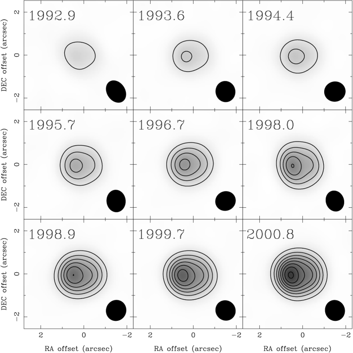
Figure 6: Diffraction-limited 9 GHz images of SNR 1987A at the nine epochs listed in Table 2. The false-colour range in each panel is –0.1 to $+$16.0 mJy beam^-1, while contours are at levels of 1.5, 3.0, 4.5, $\ldots$, 13.5 mJy beam^-1. The FWHM dimensions of the diffraction-limited synthesised beam for each epoch is shown at the lower-right of each panel.

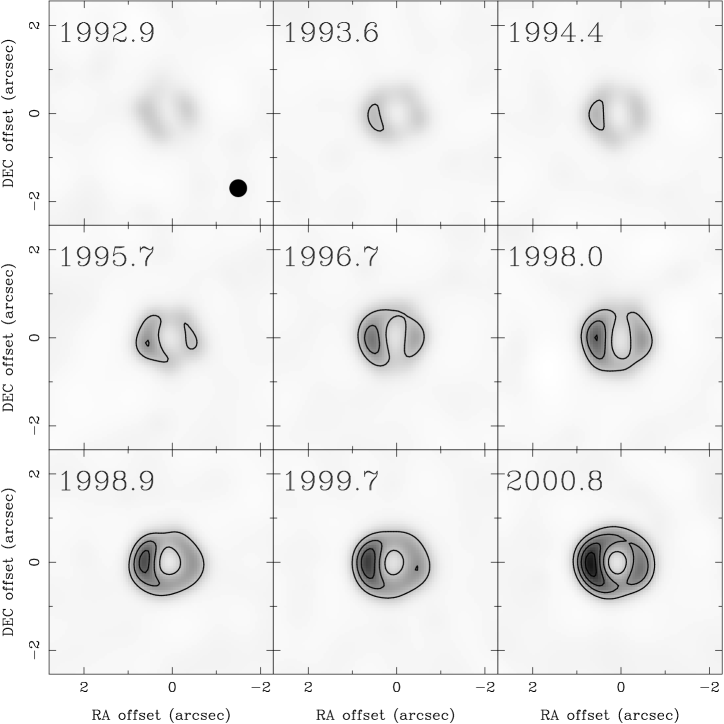
Figure 7: Super-resolved 9 GHz images of SNR 1987A at the nine epochs listed in Table 2. The false-colour range in each panel is –0.1 to $+$5.0 mJy beam^-1, while contours are at levels of 0.4, 0.8, 1.2, $\ldots$, 2.8 mJy beam^-1. The FWHM dimensions of the super-resolved synthesised beam is shown at the lower-right of the first panel.

3.2 Model Fits to the Radio Morphology

Gaensler et al. (1997) showed that the size of SNR 1987A could be quantified at each epoch by approximating the morphology of SNR 1987A by a thin spherical shell of arbitrary position, flux and radius. The best-fit parameters are found by computing the Fourier-transform of this shell, subtracting this transform from the $u-v$ data, and then adjusting the properties of the model until the corresponding $\chi^{2}$ parameter is minimised (see also Staveley-Smith et al. 1993b). Using such an approach, Gaensler et al. (1997) were able to show that the radius of the supernova remnant increased from 0$.\!\!^{\prime\prime}$65 at epoch 1992.9 to 0$.\!\!^{\prime\prime}$68 at epoch 1995.7, corresponding to a (surprisingly low) mean expansion velocity of $2800\pm 400$ km ${\rm s}^{-1}$ (assuming a distance to the supernova of 50 kpc).

Here we extend and expand on these attempts to quantify the changes in the radio remnant. We first fit a spherical shell to all subsequent data-sets. The resulting radii are listed in Table 2, where the uncertainty in the last quoted digit is given in parentheses. A fit to these radii gives a linear expansion rate of $3500\pm 100$ km ${\rm s}^{-1}$. The mean radius at each observing epoch is listed in Table 3 and plotted in Figure 8.

Figure 8: Inferred radius of the radio remnant SNR 1987A as a function of time. The filled points represent radii determined by fitting a thin spherical shell to the data, while open points correspond to a model involving a shell plus two point sources. The solid lines indicate the respective best-fit linear increases, while the dashed lines are extrapolations between the epoch of the supernova explosion and the time when radio emission re-appeared.

The signal-to-noise of the data presented by Gaensler et al. (1997) was too low to justify more complex fits to the data. However, we are now in a position to compare a thin spherical shell to other models. We first note that other simple spherically-symmetric models, such as face-on rings and gaussians, produce significant residuals, and are clearly inconsistent with the data. In Figure 9 we show three possible fits to the data from epoch 1998.0. In each case, we have generated an input model (shown in the first column). We have then simulated an observation of the sky-distribution corresponding to this model as follows: we Fourier-transform the model, then multiply this transform by the transfer function of the ATCA observations from this epoch to produce a set of $u-v$ tracks identical to those of the real data. We then image these visibilities in the same way as for the real data, and similarly deconvolve and super-resolve the image, to give the result shown in the second column. We also subtract the $u-v$ data corresponding to the model from the observed data, and then image the resulting visibilities to produce the residual image shown in the third column.

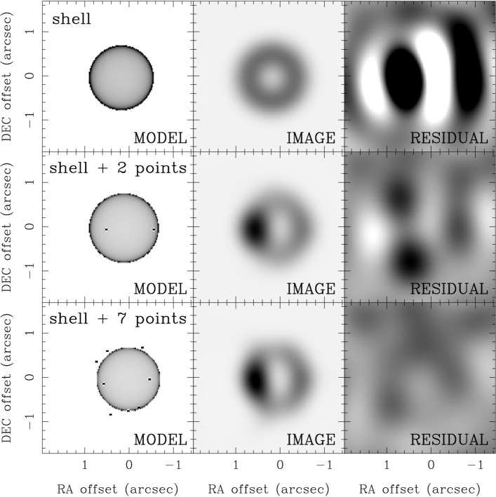
Figure 9: Models of the radio emission from SNR 1987A. Each row represents a different attempt to model the radio emission from epoch 1998.0: a thin spherical shell; a thin shell plus two hotspots; a thin shell plus seven hotspots. The first column shows the input image for each model, using a false-colour range of 0 to 0.01 mJy beam^-1; the second column shows the results of a simulated super-resolved observation of the input image, using a grayscale range of –0.16 to +3.05 mJy beam^-1; the third column shows an image of the residuals remaining once the model has been subtracted from the original data, using a false-colour range –0.2 to +0.3 mJy beam^-1. In the third model, the east point source within the shell has a flux density of 3.5 mJy; the other six have flux densities in the range 0.3 to 0.8 mJy.

In the first row of Figure 9, we show the results of fitting a thin spherical shell to the 1998.0 data (cf. Gaensler et al. 1997) — the corresponding best-fit flux and radius are 18.4 mJy and 0$.\!\!^{\prime\prime}$73. The resulting image successfully approximates the limb-brightened morphology seen in Figure 7, but lacks the enhancements in brightness seen on either side of the shell. The residual image, while having small amplitudes in an absolute sense, shows clear and systematic differences between this simple model and the data (maximum fractional residual of $\sim$20%).

Given that the main difference between a thin shell model and the data seems to be the presence of the bright lobes on either side, we next generate a model involving a thin shell (of arbitrary flux, position and radius), and two point-sources of emission (each of arbitrary flux and position). For the 1998.0 data set, the best-fit parameters for this model are a shell of flux 15.0 mJy and radius 0$.\!\!^{\prime\prime}$79, and point-sources of fluxes 3.1 and 0.4 mJy, one projected near the edge of, but inside, the eastern half of the shell, and the other similarly positioned on the western half. Note that the radius of the shell in this fit is 8% larger than that obtained by fitting to a shell alone. The resulting model, image and residual are all shown in the second row of Figure 9. The image corresponding to the model now reasonably approximates the morphology seen in the real data, and the residuals are greatly reduced (maximum fractional residual of $\sim$5%) when compared to the case of a shell alone.

We can further improve the fit between the model and the data by increasing the number of point sources in the model. In the bottom row of Figure 9, we show a fit to the 1998.0 data involving a spherical shell plus seven point sources. The large number of free parameters (25 in this case) makes finding an absolute minimum in $\chi^{2}$ very difficult — thus the “best fit” we have shown was found by trial-and-error. The shell has flux density 11.4 mJy and radius 0$.\!\!^{\prime\prime}$72 (2% smaller than in the case of a shell alone); the point sources range in flux density between 0.3 and 3.5 mJy, and are distributed around the perimeter of the shell. The model image and residual image both indicate a very good match between the model and the data (maximum fractional residual $\sim$2%). We emphasise, though, that we make no claims to uniqueness for this solution.

Table 3: Parameters from model fits to the 9 GHz images

Mean	Total Flux	Fit to shell alone		Fit to shell $+$ 2 points
Epoch	Density	$S_{\rm shell}$	$r_{\rm shell}$	$S_{\rm shell}$	$r_{\rm shell}$	$S_{\rm 1}$	$\delta{\rm RA}_{1}$	$\delta{\rm Dec}_{1}$	$S_{\rm 2}$	$\delta{\rm RA}_{2}$	$\delta{\rm Dec}_{2}$
	(mJy)	(mJy)	(′′)	(mJy)	(′′)	(mJy)	(′′)	(′′)	(mJy)	(′′)	(′′)
1992.9	5.6(2)	5.2	0.668(9)	$\ldots$	$\ldots$	$\ldots$	$\ldots$	$\ldots$	$\ldots$	$\ldots$	$\ldots$
1993.6	6.9(2)	6.6	0.659(6)	5.1	0.73(2)	1.2	0.26(3)	-0.05(2)	0.4	-0.73(9)	0.06(5)
1994.4	7.5(1)	7.8	0.671(4)	6.2	0.75(2)	1.3	0.27(2)	-0.03(1)	0.4	-0.69(7)	0.06(4)
1995.7	11.8(1)	11.0	0.684(4)	8.6	0.71(2)	1.9	0.35(3)	-0.03(1)	0.5	-0.76(8)	0.04(5)
1996.7	15.5(1)	15.1	0.688(2)	12.4	0.764(7)	2.5	0.32(1)	0.03(1)	0.4	-0.69(6)	0.15(3)
1998.0	18.3(1)	18.4	0.731(2)	15.0	0.786(8)	3.1	0.34(1)	-0.02(1)	0.4	-0.75(7)	-0.02(5)
1998.9	21.7(1)	21.5	0.730(2)	17.2	0.778(6)	3.4	0.40(1)	-0.02(1)	1.0	-0.81(3)	-0.04(2)
1999.7	24.7(1)	24.4	0.742(2)	19.7	0.796(6)	3.9	0.41(1)	-0.02(1)	1.0	-0.81(3)	-0.05(2)
2000.8	30.8(1)	30.8	0.761(2)	24.9	0.804(4)	4.8	0.46(1)	-0.01(1)	1.3	-0.82(2)	-0.03(2)

Given the difficulty in finding a multiple-component fit to the data by trial-and-error, and the non-uniqueness of this solution, we do not here present multi-parameter fits to other epochs such as those shown in the third row of Figure 9. However, it seems clear that a shell alone is no longer the best simple model of the data, and that a shell with two point-sources is a significant improvement. We therefore have fitted all epochs with these two models, with all parameters free to vary in each case. The results of these fits are listed in Table 3 and plotted in Figure 8. Offsets of the two point sources in Table 3 are with respect to the reference position used for Figures 6, 7 & 9. The data from epoch 1992.9 is of low signal-to-noise, and no good fit using this more complex model cound be found.

It can be seen from Table 3 that the radius of the shell in models which include two point-sources is 5–10% larger than that obtained in the shell-only model used by Gaensler et al. (1997). It is also clear that the point sources are moving outward with the expansion of the shell, the eastern one apparently at a larger relative rate than the shell. As for the shell model, we can fit these larger radii by a linear increase, to obtain an expansion speed of $2300\pm 300$ km ${\rm s}^{-1}$, about 35% slower than in the case for the shell alone. However, we note that if multi-parameter fits like those in the third row of Figure 9 are carried out for other epochs, the resulting radii are $\sim$5% smaller than for the fits to a shell alone, and the resulting inferred expansion speed is $\sim 3700$ km ${\rm s}^{-1}$. While we have not carried out the corresponding analysis here, we note that Staveley-Smith et al. (1993a) fitted the radio emission from SNR 1987A with a thick spherical shell of outer-to-inner radius ratio 1.25. This results in a shell diameter about 10% greater than for the thin-shell fit, consistent with the range of possible radii considered here.

We therefore conclude that the radius of the remnant as determined from fitting to the $u-v$ data is uncertain by $\sim$10%, and that the resulting expansion velocity is uncertain by $\sim$30%. The main conclusions from earlier results — that the radio emission is originating from a region within the equatorial ring, and that the material producing this emission was initially moving rapidly but now has a very low rate of expansion — are unchanged, even when the assumption of spherical symmetry is relaxed.

3.3 Comparison With Other Wavelengths and Discussion

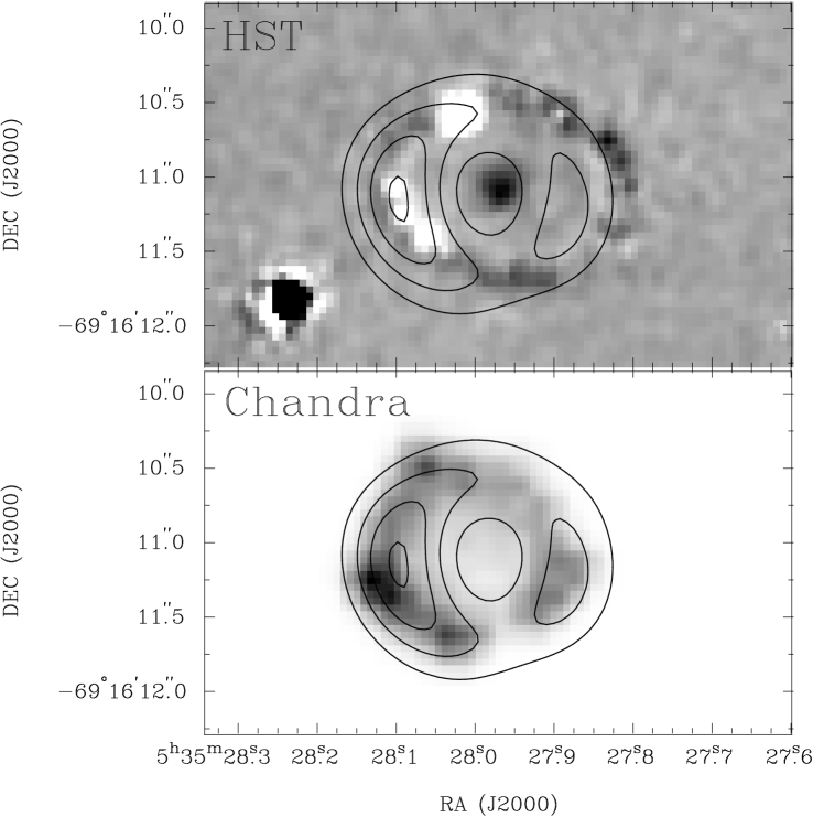
Figure 10: Multi-wavelength comparisons of SNR 1987A. The upper panel overlays HST and ATCA observations of SNR 1987A: the false-colour image represents the difference of HST WFPC2 images in the F6565N filter, obtained by subtracting an image taken in 1998 February from a similar image taken in 1999 April (Lawrence et al. 2000), while the contours correspond to the super-resolved 2000.8-epoch ATCA image, using contour levels of 1.1, 2.2, 3.3 and 4.4 mJy beam^-1. The lower panel overlays Chandra and ATCA observations — the false-colour represents a super-resolved Chandra ACIS-S image covering the energy range 0.3–8 keV at epoch 1999.8 (Burrows et al. 2000), while the contours indicate radio data as in the upper panel.

In Figure 10 we compare our 9 GHz ATCA data to recent observations with HST and with Chandra. In the upper panel, the super-resolved ATCA image from epoch 2000.8 is compared to the difference-image of optical emission around the supernova produced by Lawrence et al. (2000). The HST image has been registered on the radio frame with an accuracy of better than $0\hbox{$.\!\!^{\prime\prime}$}1$ using the position of the central star from Reynolds et al. (1995). It shows both the fading equatorial ring, and and at least seven hotspots on this ring, all brightening as the supernova shock begins to interact with dense circumstellar material. It can be seen from this optical/radio comparison that the conclusions made by Gaensler et al. (1997) are maintained: the bright radio lobes align with the major axis of the optical ring, with the brighter eastern lobe clearly more distant from the central star than the fainter western lobe. Within the uncertainties, the eastern radio lobe is coincident with some of the optical hotspots (but not the brighest one), just inside the optical ring. In the west, the optical emission lies outside the radio lobe, close to the lowest radio contour in Figure 10. In fact, there is a good correspondence of the radio emission with optical emission within the optical ring (not visible in Figure 10) corresponding to the reverse-shock, as reported by Garnavich, Kirshner & Challis (1999). Just as in the radio data, two optical lobes are seen, one to the east and one to the west of the supernova site. Also similar to the case in the radio, the eastern optical lobe is brighter than and further from the supernova than the western lobe.

The lower panel of Figure 10 compares radio emission with a super-resolved image obtained by Chandra at epoch 1999.8 (Burrows et al. 2000). The X-ray and radio emission from the supernova remnant both take the form of limb-brightened shells; the images were aligned by placing the estimated centre of the X-ray remnant on the Reynolds et al. (1995) position (D. Burrows, private communication) and hence is less accurate than the optical–radio alignment. While there is a good correspondence between the brightest regions in each waveband, the X-ray maxima appear to lie outside the radio maxima. This is perhaps surprising since theoretical models (e.g. Borkowski, Blondin & McCray 1997) suggest that the radio emission is generated just inside the outer shock whereas the X-ray emission is generated by a reverse shock compressing and heating the denser ejecta as it propagates inwards. It is worth noting, however, that X-ray emission lying outside the radio emission and interpreted as coming from the outer shock has been detected in the SNR 1E 0102.2$-$7219 by Gaetz et al. (2000).

The two-lobed radio morphology seen for SNR 1987A was apparent at least as early as 1992 (Figure 7; Staveley-Smith et al 1993a), while optical hotspots did not begin to appear on the eastern side of the optical ring until 1995 and on the western side until 1998 (Lawrence et al. 2000). Furthermore, the earliest-appearing and brightest optical hotspot does not coincide in position angle with either of the two main radio lobes, nor with the brightest X-ray emission seen by Chandra (Figure 10; Burrows et al. 2000). We therefore argue that the more rapid rate in the increase of radio emission beginning around day 3000, as reported by Ball et al. (2001) and confirmed in Section 2 above, is not related to the appearance of optical hotspots seen at around the same time. While Ball et al. (2001) have pointed out that the various optical hotspots turned on at about the right time for them to have been produced by the arrival of the radio-producing shock(s) in these regions, it seems clear that this had little effect on the radio morphology of the remnant. The best explanation for deviations from spherical symmetry in the radio morphology of SNR 1987A still seems to be that they result simply from regions of enhanced emission in the equatorial plane of the progenitor system, where circumstellar gas is expected to be both densest and closest to the progenitor star (cf. Gaensler et al. 1997). The fact that at both radio and optical wavelengths the eastern lobe is both brighter and more distant from the explosion site than the western lobe may represent an asymmetry in the distribution of ejecta.

It is notable that the emission underlying the radio hotspots is well described by a spherical shell and that, in all of the models, the flux density of the shell dominates the total flux density. This is surprising given the strong equatorial enhancement evident in the optical data and implied for the circumstellar gas. One might expect eventually to see a faster expansion of the radio remnant in the polar directions (Blondin, Lundqvist & Chevalier 1996), but there is currently no evidence for this. Part of the radio emission from the lobes may be attributed to an equatorial enhancement but, since such an enhancement would be symmetric, it cannot account for all of the emission seen from the brighter eastern lobe. It is worth noting that the shell of SN 1993J also appears to be quite spherical (Marcaide et al. 1997, Bartel et al. 2000).

4 Future Prospects

Results at all wavelengths suggest that there is an increasing interaction between the expanding ejecta and the circumstellar material. Hotspots around or just inside the emission-line ring are certainly becoming more numerous and prominent in the optical band. Neither the radio imaging nor the X-ray imaging has sufficient resolution to separately identify hot spots. However, the modelling of the radio $u-v$ data and the possible short-term fluctuations in the rise of the high-frequency radio flux densities suggest that compact radio hotspots do exist. The overall morphology and the time-evolution of the radio emission suggest that there is no detailed correspondence of the radio hotspots with the hotspots seen in the optical data and, in fact, that the radio hotspots are much more numerous and widespread.

We have shown that the rate of increase of the radio emission from SNR 1987A has slowly increased over the past few years. It is possible that the rate of increase of the radio (and other) emission will dramatically increase when significant amounts of ejecta begin to interact with the dense circumstellar gas of the inner ring. Extrapolation of the radii and expansion speeds resulting model fits to the radio data suggest that this will happen in $2004\pm 2$. The ATCA is presently being upgraded for observations in the 12 mm and 3 mm bands, with an expected commissioning date of mid-2002. While the radio remnant is unlikely to be detectable at 3 mm, we expect 12 mm observations to provide increased resolution. Extrapolating the present flux density increase and the currently observed power-law spectrum, we expect a flux density at 20 GHz in mid-2002 of about 17 mJy. The diffraction limited half-power beamwidth at 20 GHz will be about 0$.\!\!^{\prime\prime}$4, somewhat less than the present super-resolved beamwidth at 9 GHz. Even in 2002, it is likely that super-resolution will be able to be applied to the 20 GHz data, giving a resolution of about 0$.\!\!^{\prime\prime}$2, and this will certainly be true at later epochs if the flux density continues to rise. We hope and expect that this will reveal further detail in the radio images, allowing interesting comparisons with images obtained at other wavelengths and giving further insight into the physics of the radio emission process.

References

Ball, L., Campbell-Wilson, D., Crawford, D. F., & Turtle, A. J. 1995, ApJ, 453, 864

Ball, L., Crawford, D. F., Hunstead, R. W., Klamer, I., & McIntyre, V. J. 2001, ApJ, 549, 599

Ball, L. & Kirk, J. G. 1992, ApJ Lett., 396, L39

Baring, M. G., Ellison, D. C., Reynolds, S. P., Grenier, I. A., & Goret, P. 1999, ApJ, 513, 311

Bartel, N. et al. 2000, Science, 287, 112

Blondin, J. M., Lundqvist, P. & Chevalier, R. A., 1996, ApJ, 472, 257

Borkowski, K. J., Blondin, J. M. & McCray, R. 1997, ApJ, 476, L31

Briggs, D. S. 1994, in The Restoration of HST Images and Spectra II, ed. R. J. Hanisch & R. L. White, (Baltimore: Space Telescope Science Institute), 250

Burrows, C. J. et al. 1995, ApJ, 452, 680

Burrows, D. N. et al. 2000, ApJ, 543, L149

Chevalier, R. A. 1992, Nature, 355, 617

Chevalier, R. A. & Dwarkadas, V. V. 1995, ApJ, 452, L45

Chevalier, R. A. & Fransson, C. 1987, Nature, 328, 44

Crotts, A. P. S., Kunkel, W. E., & Heathcote, S. R. 1995, ApJ, 438, 724

Duffy, P., Ball, L., & Kirk, J. G. 1995, ApJ, 447, 364

Gaensler, B. M., Manchester, R. N., Staveley-Smith, L., Tzioumis, A. K., Reynolds, J. E., & Kesteven, M. J. 1997, ApJ, 479, 845

Gaetz, T. J., Butt, Y. M., Edgar, R. J., Eriksen, K. A., Plucinsky, P. P., Schlegel, E. M. & Smith, R. K. 2000, ApJ, 534, L47

Garnavich, P., Kirshner, R., & Challis, P. 1999. IAU Circ. 7102

Gorenstein, P., Hughes, J. P., & Tucker, W. H. 1994, ApJ, 420, L25

Green, D. A. 2000, A Catalogue of Galactic Supernova Remnants, (Cambridge: Mullard Radio Astronomy Observatory, Cavendish Laboratory). http://www.mrao.cam.ac.uk/surveys/snrs/.

Hasinger, G., Aschenbach, B., & Trümper, J. 1996, A&A, 312, L9

Jauncey, D. L., Kemball, A., Bartel, N., Shapiro, I. I., Whitney, A. R., Rogers, A. E. E., Preston, R. A., & Clark, T. 1988, Nature, 334, 412

Jones, F. C. & Ellison, D. C. 1991, Space Sci. Rev., 58, 259

Lawrence, S. S., Sugerman, B. E., Bouchet, P., Crotts, A. P. S., Uglesich, R., & Heathcote, S. 2000, ApJ, 537, L123

Marcaide, J. E. et al. 1997, ApJ, 486, L31

Montes, M. J., van Dyk, S. D., Weiler, K. W., Sramek, R. A., & Panagia, N. 1998, ApJ, 506, 874

Montes, M. J., Weiler, K. W., Van Dyk, S. D., Panagia, N., Lacey, C. K., Sramek, R. A., & Park, R. 2000, ApJ, 532, 1124

Plait, P. C., Lundqvist, P., Chevalier, R. A., & Kirshner, R. P. 1995, ApJ, 439, 730

Pun, C. S. J., Sonneborn, G., Bowers, C., Gull, T., Heap, S., Kimble, R., Maran, S., & Woodgate, B. 1997. IAU Circ. 6665

Reynolds, J. E. et al. 1995, A&A, 304, 116

Reynolds, S. P. & Ellison, D. C. 1992, ApJ, 399, L75

Spyromilio, J., Stathakis, R. A. & Meurer, G. R. 1993, MNRAS, 263, 530

Spyromilio, J. 1994, MNRAS, 266, 61

Staveley-Smith, L., Manchester, R. N., Kesteven, M. J., Campbell-Wilson, D., Crawford, D. F., Turtle, A. J., Reynolds, J. E., Tzioumis, A. K., Killeen, N. E. B. & Jauncey, D. L. 1992, Nature, 355, 147

Staveley-Smith, L., Briggs, D. S., Rowe, A. C. H., Manchester, R. N., Reynolds, J. E., Tzioumis, A. K., & Kesteven, M. J. 1993a, Nature, 366, 136

Staveley-Smith, L., Manchester, R. N., Kesteven, M. J., Tzioumis, A. K., & Reynolds, J. E. 1993b, PASA, 10, 331.

Storey, M. C. & Manchester, R. N. 1987, Nature, 329, 421

Turtle, A. J. et al. 1987, Nature, 327, 38

van Dyk, S. D., Weiler, K. W., Sramek, R. A., Rupen, M. P., & Panagia, N. 1994, ApJ, 432, L115

Weiler, K. W., van Dyk, S. D., Montes, M. J., Panagia, N., & Sramek, R. A. 1998, ApJ, 500, 51

Appendix

Table 4 gives flux densities measured at the four ATCA frequencies over the day range 2000 - 5100 (MJD 48449 to 51949). These are calibrated relative to the primary flux calibrator, PKS B1934-638, using standard techniques. This table, also including flux density measurements for the nearby unresolved source J0536-6918 and more recent measurements, is available at http://www.atnf.csiro.au/research/pulsar/snr/sn1987a/.

Table 4: ATCA flux density measurements for SNR 1987A

1.4 GHz		2.4 GHz		4.8 GHz		8.6 GHz
Day	Flux Density	Day	Flux Density	Day	Flux Density	Day	Flux Density
Number	(mJy)	Number	(mJy)	Number	(mJy)	Number	(mJy)
1243.9	$0.00\pm 1.20$	1198.9	$0.00\pm 1.00$	1243.6	$0.00\pm 0.25$	1388.1	$1.33\pm 0.26$
1270.7	$2.92\pm 1.20$	1314.5	$3.27\pm 1.00$	1269.7	$0.66\pm 0.25$	1432.2	$1.12\pm 0.26$
1386.4	$4.87\pm 1.21$	1386.0	$3.45\pm 1.01$	1305.5	$1.15\pm 0.25$	1500.5	$1.74\pm 0.26$
1490.0	$7.61\pm 1.22$	1517.9	$6.13\pm 1.02$	1333.7	$1.49\pm 0.26$	1515.0	$2.34\pm 0.28$
1517.9	$8.29\pm 1.23$	1517.7	$6.20\pm 1.02$	1366.3	$1.53\pm 0.26$	1583.8	$2.62\pm 0.28$
1517.7	$9.55\pm 1.23$	1595.8	$5.55\pm 1.01$	1385.2	$1.96\pm 0.26$	1593.8	$2.21\pm 0.27$
1595.8	$10.15\pm 1.24$	1636.7	$8.71\pm 1.03$	1401.4	$2.17\pm 0.26$	1662.5	$2.92\pm 0.29$
1636.7	$15.52\pm 1.29$	1660.5	$9.15\pm 1.04$	1402.4	$2.15\pm 0.26$	1661.5	$2.50\pm 0.28$
1660.5	$15.52\pm 1.29$	1788.8	$10.67\pm 1.05$	1403.4	$2.25\pm 0.27$	1786.6	$3.92\pm 0.32$
1788.8	$20.59\pm 1.35$	1850.1	$13.07\pm 1.07$	1404.3	$2.12\pm 0.26$	1852.1	$4.37\pm 0.33$
1850.1	$24.80\pm 1.41$	1879.2	$15.03\pm 1.10$	1405.3	$2.13\pm 0.26$	1878.2	$4.14\pm 0.32$
1879.2	$24.04\pm 1.40$	1969.7	$17.95\pm 1.14$	1407.1	$2.06\pm 0.26$	1947.8	$4.70\pm 0.34$
1969.7	$27.51\pm 1.46$	2067.7	$19.00\pm 1.15$	1408.3	$2.57\pm 0.27$	1969.5	$4.93\pm 0.35$
2068.4	$33.15\pm 1.56$	2313.7	$23.25\pm 1.22$	1409.3	$2.53\pm 0.27$	1986.4	$4.64\pm 0.34$
2313.7	$38.87\pm 1.67$	2427.3	$23.37\pm 1.22$	1410.3	$2.66\pm 0.27$	2003.4	$5.09\pm 0.36$
2427.3	$39.96\pm 1.70$	2505.2	$25.91\pm 1.27$	1431.2	$2.29\pm 0.27$	2067.5	$5.48\pm 0.37$
2505.2	$43.23\pm 1.77$	2549.2	$26.56\pm 1.28$	1446.2	$2.63\pm 0.27$	2092.4	$5.92\pm 0.39$
2549.2	$43.83\pm 1.78$	2680.7	$28.40\pm 1.31$	1460.1	$3.03\pm 0.28$	2142.2	$5.43\pm 0.37$
2680.7	$46.20\pm 1.83$	2774.5	$29.92\pm 1.34$	1516.9	$2.83\pm 0.27$	2195.7	$4.20\pm 0.33$
2774.5	$49.26\pm 1.90$	2773.7	$30.40\pm 1.35$	1524.9	$2.74\pm 0.27$	2261.8	$6.04\pm 0.39$
2773.7	$48.60\pm 1.89$	2826.7	$28.40\pm 1.31$	1586.8	$2.97\pm 0.28$	2299.9	$7.14\pm 0.44$
2857.7	$50.90\pm 1.94$	2857.7	$29.30\pm 1.33$	1594.8	$4.50\pm 0.31$	2299.7	$5.80\pm 0.38$
2874.3	$48.40\pm 1.88$	2874.3	$25.20\pm 1.25$	1635.6	$5.31\pm 0.33$	2313.7	$6.92\pm 0.43$
2919.2	$53.77\pm 2.01$	2919.2	$33.11\pm 1.41$	1662.5	$5.02\pm 0.32$	2320.7	$6.90\pm 0.43$
2919.3	$51.38\pm 1.95$	2919.3	$34.20\pm 1.43$	1746.8	$6.04\pm 0.35$	2374.7	$5.38\pm 0.37$
2975.8	$54.97\pm 2.04$	2975.8	$33.55\pm 1.42$	1786.8	$7.44\pm 0.39$	2403.5	$7.14\pm 0.44$
2975.7	$48.40\pm 1.88$	2975.7	$32.50\pm 1.40$	1852.1	$8.16\pm 0.41$	2426.4	$7.68\pm 0.46$
3001.7	$48.80\pm 1.89$	3001.7	$33.11\pm 1.41$	1878.2	$7.06\pm 0.38$	2462.7	$6.50\pm 0.41$
3000.7	$56.20\pm 2.07$	3072.5	$34.60\pm 1.44$	1947.8	$8.27\pm 0.41$	2550.2	$7.47\pm 0.45$
3072.5	$61.70\pm 2.21$	3139.7	$36.60\pm 1.49$	1969.5	$9.11\pm 0.44$	2572.0	$5.93\pm 0.39$
3072.5	$57.20\pm 2.09$	3176.7	$35.90\pm 1.47$	1986.4	$8.44\pm 0.42$	2579.8	$6.92\pm 0.43$
3139.7	$61.00\pm 2.19$	3202.7	$39.20\pm 1.54$	2003.4	$8.72\pm 0.43$	2579.7	$6.50\pm 0.41$
3176.7	$59.10\pm 2.14$	3277.7	$41.60\pm 1.60$	2067.2	$9.42\pm 0.45$	2628.0	$9.00\pm 0.51$

Table 4: – continued

1.4 GHz		2.4 GHz		4.8 GHz		8.6 GHz
Day	Flux Density	Day	Flux Density	Day	Flux Density	Day	Flux Density
Number	(mJy)	Number	(mJy)	Number	(mJy)	Number	(mJy)
3202.7	$64.20\pm 2.27$	3325.7	$41.40\pm 1.59$	2092.4	$9.94\pm 0.47$	2627.7	$7.80\pm 0.46$
3277.7	$66.20\pm 2.32$	3414.8	$44.10\pm 1.66$	2142.5	$8.56\pm 0.42$	2647.7	$6.10\pm 0.39$
3325.7	$67.10\pm 2.34$	3455.7	$44.80\pm 1.68$	2195.7	$9.10\pm 0.44$	2754.8	$6.26\pm 0.40$
3414.8	$71.80\pm 2.47$	3515.4	$45.80\pm 1.70$	2261.8	$10.86\pm 0.50$	2753.7	$5.40\pm 0.37$
3455.7	$71.80\pm 2.47$	3579.2	$48.50\pm 1.77$	2299.9	$11.50\pm 0.52$	2774.5	$9.22\pm 0.52$
3515.4	$73.30\pm 2.51$	3633.1	$48.00\pm 1.75$	2299.7	$11.60\pm 0.53$	2826.7	$9.80\pm 0.55$
3579.2	$77.50\pm 2.62$	3679.0	$49.40\pm 1.79$	2374.7	$10.82\pm 0.50$	2919.2	$9.44\pm 0.53$
3633.1	$79.10\pm 2.66$	3714.0	$50.10\pm 1.81$	2403.5	$12.42\pm 0.56$	2919.3	$11.30\pm 0.62$
3679.0	$79.60\pm 2.67$	3744.7	$48.50\pm 1.77$	2462.7	$12.80\pm 0.57$	2975.8	$9.11\pm 0.52$
3714.0	$79.30\pm 2.66$	3771.6	$49.90\pm 1.80$	2511.0	$11.98\pm 0.54$	2975.7	$8.30\pm 0.48$
3744.7	$84.40\pm 2.80$	3833.6	$50.10\pm 1.81$	2572.0	$13.99\pm 0.61$	3000.7	$6.60\pm 0.41$
3771.6	$81.90\pm 2.73$	3900.3	$52.60\pm 1.87$	2579.8	$13.62\pm 0.60$	3001.7	$9.23\pm 0.52$
3833.6	$84.20\pm 2.80$	3945.4	$52.20\pm 1.86$	2579.7	$13.10\pm 0.58$	3072.5	$10.40\pm 0.58$
3900.3	$86.00\pm 2.85$	3987.1	$52.40\pm 1.86$	2628.0	$13.53\pm 0.60$	3073.6	$11.40\pm 0.62$
3945.4	$88.10\pm 2.90$	4015.1	$55.30\pm 1.94$	2627.7	$14.10\pm 0.62$	3110.6	$10.20\pm 0.57$
3987.1	$93.80\pm 3.06$	4058.5	$58.30\pm 2.01$	2647.7	$12.90\pm 0.57$	3176.7	$9.80\pm 0.55$
4015.1	$89.30\pm 2.94$	4100.8	$58.30\pm 2.01$	2754.8	$14.17\pm 0.62$	3202.7	$12.60\pm 0.68$
4058.5	$87.70\pm 2.89$	4169.5	$61.40\pm 2.10$	2753.7	$13.61\pm 0.60$	3277.7	$12.10\pm 0.65$
4100.8	$96.70\pm 3.14$	4222.5	$59.20\pm 2.04$	2774.5	$14.63\pm 0.64$	3325.7	$11.70\pm 0.64$
4169.5	$99.60\pm 3.22$	4291.4	$64.70\pm 2.18$	2773.7	$14.10\pm 0.62$	3414.8	$11.50\pm 0.63$
4222.5	$97.50\pm 3.16$	4373.1	$62.30\pm 2.12$	2826.7	$14.50\pm 0.63$	3436.7	$15.70\pm 0.82$
4291.4	$104.50\pm 3.36$	4424.0	$67.10\pm 2.25$	2919.2	$16.47\pm 0.70$	3455.7	$14.20\pm 0.75$
4373.1	$108.30\pm 3.46$	4460.9	$68.90\pm 2.30$	2919.3	$16.10\pm 0.69$	3485.5	$16.10\pm 0.84$
4424.0	$107.40\pm 3.44$	4539.8	$75.50\pm 2.48$	2975.8	$15.28\pm 0.66$	3512.4	$16.50\pm 0.86$
4460.9	$113.20\pm 3.60$	4571.7	$69.50\pm 2.31$	2975.7	$16.50\pm 0.71$	3515.4	$14.60\pm 0.77$
4539.8	$112.60\pm 3.58$	4684.9	$75.20\pm 2.47$	3000.7	$15.10\pm 0.65$	3579.2	$15.50\pm 0.81$
4571.7	$116.10\pm 3.68$	4728.9	$74.20\pm 2.44$	3001.7	$16.84\pm 0.72$	3633.1	$14.90\pm 0.79$
4684.9	$121.20\pm 3.83$	4768.1	$77.10\pm 2.52$	3072.5	$17.80\pm 0.75$	3679.0	$16.30\pm 0.85$
4728.9	$121.40\pm 3.83$	4799.9	$77.40\pm 2.53$	3176.7	$16.90\pm 0.72$	3714.0	$15.90\pm 0.83$
4768.1	$131.30\pm 4.12$	4837.9	$83.80\pm 2.71$	3202.7	$20.20\pm 0.85$	3744.7	$16.30\pm 0.85$
4799.9	$124.90\pm 3.93$	4850.8	$77.80\pm 2.54$	3277.7	$21.60\pm 0.90$	3771.6	$17.90\pm 0.93$
4837.9	$126.40\pm 3.98$	4870.7	$77.90\pm 2.54$	3325.7	$20.70\pm 0.86$	3833.6	$17.70\pm 0.92$
4850.8	$128.70\pm 4.04$	4936.5	$81.00\pm 2.63$	3414.8	$21.30\pm 0.89$	3900.3	$17.10\pm 0.89$
4870.7	$127.00\pm 3.99$	4997.3	$83.60\pm 2.70$	3455.7	$23.10\pm 0.96$	3945.4	$17.90\pm 0.93$
4936.5	$133.40\pm 4.18$	5024.8	$83.00\pm 2.68$	3515.4	$24.80\pm 1.02$	3987.1	$18.90\pm 0.98$
4997.3	$136.90\pm 4.28$	5050.1	$86.20\pm 2.77$	3579.2	$25.40\pm 1.05$	4015.1	$19.40\pm 1.00$
5024.8	$135.00\pm 4.22$	5093.0	$86.60\pm 2.78$	3633.1	$25.10\pm 1.03$	4100.8	$19.60\pm 1.01$
5050.1	$135.90\pm 4.25$			3679.0	$24.50\pm 1.01$	4222.5	$19.10\pm 0.99$
5093.0	$143.40\pm 4.47$			3714.0	$24.50\pm 1.01$	4291.4	$21.00\pm 1.08$
				3744.7	$27.00\pm 1.11$	4373.1	$21.20\pm 1.09$
				3771.6	$27.10\pm 1.11$	4424.0	$24.90\pm 1.27$
				3833.6	$26.50\pm 1.09$	4460.9	$25.50\pm 1.30$

Table 4: – continued

1.4 GHz		2.4 GHz		4.8 GHz		8.6 GHz
Day	Flux Density	Day	Flux Density	Day	Flux Density	Day	Flux Density
Number	(mJy)	Number	(mJy)	Number	(mJy)	Number	(mJy)
				3900.3	$29.20\pm 1.19$	4539.8	$25.00\pm 1.27$
				3945.4	$29.80\pm 1.22$	4571.7	$24.40\pm 1.25$
				3987.1	$31.90\pm 1.30$	4684.9	$26.70\pm 1.36$
				4015.1	$30.20\pm 1.23$	4728.9	$28.10\pm 1.43$
				4100.8	$32.00\pm 1.30$	4768.1	$25.70\pm 1.31$
				4222.5	$32.00\pm 1.30$	4799.9	$24.80\pm 1.26$
				4291.4	$35.30\pm 1.43$	4837.9	$31.50\pm 1.59$
				4424.0	$34.10\pm 1.39$	4850.8	$27.90\pm 1.42$
				4460.9	$38.60\pm 1.56$	4870.7	$29.90\pm 1.52$
				4539.8	$37.60\pm 1.52$	4936.5	$30.20\pm 1.53$
				4571.7	$39.60\pm 1.60$	4997.3	$27.50\pm 1.40$
				4684.9	$40.10\pm 1.62$	5024.8	$31.90\pm 1.61$
				4728.9	$43.70\pm 1.77$	5050.1	$31.90\pm 1.61$
				4768.1	$42.70\pm 1.73$	5093.0	$36.00\pm 1.82$
				4799.9	$39.70\pm 1.61$
				4837.9	$43.60\pm 1.76$
				4850.8	$45.50\pm 1.84$
				4870.7	$47.20\pm 1.90$
				4936.5	$48.10\pm 1.94$
				4997.3	$43.50\pm 1.76$
				5024.8	$47.70\pm 1.92$
				5050.1	$46.40\pm 1.87$
				5093.0	$49.90\pm 2.01$