On the shear instability of fluid interfaces:
Stability analysis

Abstract

We examine the linear stability of fluid interfaces subjected to a shear flow. Our main object is to generalize previous work to arbitrary Atwood number, and to allow for surface tension and weak compressibility. The motivation derives from instances in astrophysical systems where mixing across material interfaces driven by shear flows may significantly affect the dynamical evolution of these systems.

I Introduction

The stability of fluid interfaces in the presence of shear flows has been studied for almost half a century; and was largely motivated by the problem of accounting for observations of surface water waves in the presence of winds. As early as the 1950’s, it was realized that classical Kelvin-Helmholtz instability [3] could not account for the observed water waves (cf. [20, 18]), and efforts were initiated to study the full range of possible unstable modes by which interfaces such as represented by the water/air interface could become unstable. By the early 1960’s, the basic mechanism was understood, largely on the basis of work by Miles [21, 22, 23] and Howard [13]: They discovered that interface waves for which gravity provided the restoring force (e.g., waves that can be identified with so-called deep water waves) can be driven unstable via a resonant interaction with the ambient wind; this work was also one of the first applications in which resonant (or critical) layers played an essential role in both the physics and the mathematics. Work carried out at that time showed that the precise form of the vertical wind shear profile was critical to the nature of the instability; typically, it was assumed that the wind immediately above the water surface could be characterized by a logarithmic profile of the form

$$U(z)=U_{o}+U_{1}\ln(z/\delta+1)~{},$$ (1)

where $U_{o}$ is the velocity jump (if any) at the water/air interface, $z$ is the vertical coordinate (with $z=0$ marking the initial water-air interface), and $\delta$ is the characteristic scale length of the shear flow in the air. The idea was then to demonstrate that surface gravity waves whose phase speed is given by $c=\sqrt{g\lambda A}$ ($g$ the gravitational acceleration, $\lambda$ the perturbation mode wavelength, and $A\equiv(\rho_{2}-\rho_{1})/(\rho_{2}+\rho_{1})$ the Atwood number for a density interface between fluids of density $\rho_{1}$ [upper fluid] and $\rho_{2}$ [lower fluid], with $\rho_{1}<\rho_{2}$) can couple to this wind profile at a height $z$ where $c\sim U(z)$. At the time, it was not possible to construct a self-consistent description of the problem, such that a logarithmic wind profile automatically emerged from the analysis; and much of subsequent work has focused on establishing the nature of this wind shear profile (e.g., [25]). Finally, we note that these studies have since been applied to a number of other contexts, including especially shear flows in atmospheric boundary layers, where they have been extensively expanded, including into the weakly compressible regime [7].

Our own work is originally motivated by an astrophysical problem in which mixing at a material interface between two fluids with different densities is essential to the evolution of the astrophysical problem. Specifically, consider a white dwarf star, whose composition is almost completely dominated by carbon and oxygen. If such a star is in a close binary orbit with a normal main sequence star, then it has been known for some time (e.g., [31]) that accretion of matter from the normal star (largely in the form of hydrogen and helium) can lead to a build-up of an accretion envelope on the white dwarf which is capable of initiating nuclear hydrogen “burning”. This burning process can lead to a nuclear runaway, in which the energy released as a result of these nuclear fusion reaction is sufficient to expel a large fraction of the accreted matter in the form of a shell; such a runway is referred to in the astronomical literature as a “nova”. The key element relevant to our present discussion is then that observations show that approximately 30% by mass of the ejecta are in the form of C+O nuclei: since neither carbon nor oxygen are products of hydrogen burning in the accreted envelope, it must be the case that some sort of mixing process brought large amounts of stellar (i.e., white dwarf) carbon and oxygen into the overlying accreted material before envelope ejection. Furthermore, detailed analysis of the energetics of the runaway process has shown that simple hydrogen burning in the envelope cannot provide enough energy to power the observed nova; thus, additional energy release via “catalytic” nuclear reactions in which C+O play important roles is required in order to match the observations (cf. [32, 33, 34, 35, 30, 29]). Thus, from the perspective of both observed abundances of nova ejecta and consideration of the nova energetics, efficient mixing at the star/envelope interface is called for. Several possible mixing processes have been discussed in the literature, including undershoot driven by thermal convection in the burning envelope and Kelvin-Helmholtz instability; but detailed studies shown all of them to be ineffective in producing the required mixing (e.g.,[16, 15, 17]). In this regard, the current astrophysical situation resembles the problem encountered by oceanographers in the 1950’s, as they tried to explain the observed mixing between the sea water-atmosphere interface. A new instability is needed to account for the observed mixing [20].

Following the previous oceanographic work, we explore the possibility that a critical-layer instability related to the coupling of stellar surface gravity waves to a shear flow in the hydrogen envelope - can account for the enhanced mixing rate. Thus, in this paper we embark on a systematic study of such an instability and apply our results to the specific case of mixing of C/O to H/He envelope of white dwarf stars [28]. We note that similar scenarios can arise in a variety of other astrophysical systems, such as in the boundary layer between an accretion disk and a compact star, where mixing between fluids of different densities – as in the nova problem – is expected to play an important role. However, the earlier non astrophysical work largely focused on the case of very large density differences between the two fluids separated by an interface, and primarily considered the fully incompressible case (the weakly compressible case has been considered by [7]). For the astrophysical case, the density ratios can be of order unity (for the nova case a typical value would be $\rho_{1}/\rho_{2}\sim 1/10$) and the Mach number for the interface between the accretion flow and the white dwarfs surface can range from very subsonic to of order 0.2. The aim of this paper therefore is to extend the shear flow analysis to arbitrary density ratios , shear and compressibility. We provide estimates of the growth rates of unstable surface waves, and determine the regions in the control parameter space that correspond to different instabilities for different physical situations.

This paper is structured as follows: In the next section we define the problem to be solved more precisely; §III describes the linear analysis for the incompressible, two-layer case. §IV and §V describe, respectively, the inclusion of surface tension and extension to compressible flow of low Mach numbers. We discuss and summarize our results in the final section.

II Formulation

The starting point of our formulation is the identification of the appropriate material equations of motion. This issue has been well-discussed in the literature, including the motivating white dwarf case [6]: in general, we can expect the gaseous surface and atmosphere of such stars to be well described by the single fluid equations for an ideal gas. More specifically, the length scales of the physical mixing processes discussed here are all far larger than the Debye length, so that the ionized stellar material can be considered to be neutral; and as long as the stellar magnetic fields are weak (e.g., $\beta\equiv$ gas preassure/magnetic preassure $\gg 1$) we can ignore the Lorentz force. Furthermore, the ratio of the spatial scales of interest to the Kolmogorov scale is large (typically $>10^{4}$) so that we are in the large Reynolds number limit, and viscous effects on the motions of interest will be negligible. As a consequence, the Euler equations will be describing our system.

We consider a two-dimensional flow with $x$ the horizontal direction and $y$ the vertical. The system consists a layer of light fluid (density $\rho_{1}$) on top of a layer of heavy fluid (density $\rho_{2}$). In most of our analysis $\rho_{1}$ and $\rho_{2}$ are constant in each layer, and in the most general scenario both layers can be stratified (densities are functions of $y$). The two layers are separated by an interface given by $y=h(x;t)$, which initially is taken to be flat ($y=h(x;0)=0$). The upper layer ($\rho_{1}$) is moving with velocity $\mbox{\rm U}(y)$ in the $x$ direction parallel to the initial flat interface, while the lower layer ($\rho_{2}$) remains still.

As already mentioned, the instability of such stratified shear flow has been investigated (cf. [20, 13]), albeit under limited physical circumstances. We study this problem in full generality, allowing for a variety of effects (including broad ranges in the values of the Atwood number/gravity and in compressibility) with the motivation that one can establish the role of the relevant instabilities under more general astrophysical circumstances than the restricted case of nova-related mixing which motivated our study.

A The general problem

A wind (shear flow) is assumed to flow only in the layer of light fluid ($\rho_{1}$) and is zero in the heavy fluid ($\rho_{2}$). Within each layer, the governing equations are the continuity equation

$$\partial_{t}\rho+\nabla\cdot(\rho\vec{u})=0,$$ (2)

and the two-dimensional Euler equation

$$\rho\partial_{t}\vec{u}+\rho\vec{u}\cdot\nabla\vec{u}=-\nabla P+\rho\vec{g}.$$ (3)

The equation of state closes the system, which is expressed in dynamical terms:

$$(\partial_{t}+\vec{u}\cdot\nabla)\mbox{\rm P}=\frac{\mbox{\rm D}\mbox{\rm P}}{\mbox{\rm D}t}=\frac{\gamma\mbox{\rm P}}{\rho}\frac{\mbox{\rm D}\rho}{\mbox{\rm D}t},$$ (4)

where $\gamma$ is the polytropic exponent. The background density and pressure are in hydrostatic equilibrium, $\partial_{y}P_{o}=-\rho_{o}g$. The basic state is then defined by a shear flow $(\mbox{\rm U}(y))$ in the upper layer, and hydrostatic pressure $(P_{o})$ and density profiles $(\rho_{o})$. We perturb around this basic state

$$\vec{u}=\mbox{\rm U}(y)\hat{x}+\vec{u^{\prime}},\;\;\;\rho=\rho_{0}(y)+\rho^{\prime},\;\;\;\mbox{\rm P}=\mbox{\rm P}_{0}(y)+\mbox{\rm p}^{\prime},$$ (5)

and study the growth of the perturbations (primed variables). From equation 4, the density and pressure perturbations satisfy the relation

$$\frac{\mbox{\rm D}\mbox{\rm p}^{\prime}}{\mbox{\rm D}t}=c_{s}^{2}\frac{\mbox{\rm D}\rho^{\prime}}{\mbox{\rm D}t}+{w^{\prime}(g\rho_{0}+c_{s}^{2}\rho_{0y}}),$$ (6)

where $w^{\prime}$ is the vertical component of the perturbation velocity, $g$ is the gravitational acceleration, and $c_{s}=\sqrt{\gamma P_{0}/\rho_{0}}$ is the sound speed for the background state. Upon expanding the perturbations in normal modes $e^{ik(x-ct)}$, we obtain the linearized equations in the perturbation quantities (where we have dropped the primes for convenience):

$$\begin{array}[]{lll}ik(\mbox{\rm U}-c)u&+w\partial_{y}U&=-ik\rho_{o}^{-1}p\,,\\ ik(\mbox{\rm U}-c)w&&=-\rho_{o}^{-1}\partial_{y}p-\rho_{o}^{-1}g\rho\,,\\ ik(\mbox{\rm U}-c)\rho&&=-\rho_{o}(iku+\partial_{y}w)-w\partial_{y}\rho_{o}\,,\\ ik(\mbox{\rm U}-c)p&-wg\rho_{o}&=c_{s}^{2}\left(ik(U-c)\rho+w\partial_{y}\rho_{o}\right)\,.\end{array}$$ (7)

The above equations form an eigenvalue problem for the complex number $c$. One immediately sees that the incompressibility condition $\nabla\cdot\vec{u}=0$ can be obtained by taking the limit $c_{s}\to\infty$. Our problem simplifies greatly with this assumption. Therefore we first present our results for the incompressible case, and then examine how compressibility modifies the stability properties.

B The incompressible case

For the incompressible case we define a stream function $\Psi$ such that $u=\partial_{y}\Psi$ and $w=-\partial_{x}\Psi$. The 2-D Euler equation thus reads

$$\partial_{t}\nabla^{2}\Psi-\Psi_{x}\nabla^{2}\Psi_{y}+\Psi_{y}\nabla^{2}\Psi_{x}=0,\quad y\neq h.$$ (8)

The total stream function $\Psi=\Psi_{0}+\psi$ consists of a background stream function $\Psi_{0}=\int_{0}^{y}\mbox{\rm U}(z)dz$ and a perturbation $\psi=\phi(y)e^{ik(x-ct)}$. The linear equation for $\phi$ is the well-studied Rayleigh equation,

$$\phi^{\prime\prime}-\Big{(}k^{2}+\frac{\mbox{\rm U}^{\prime\prime}}{\mbox{\rm U}-c}\Big{)}\phi=0.$$ (9)

The boundary conditions at the interface for the continuity of the normal component of the velocity and pressure are:

$$(\mbox{\rm U}-c)\tilde{h}-\phi^{\pm} = 0,\;\;\;$$ (10)

$$\Delta\big{[}\rho_{i}((\mbox{\rm U}-c)\phi^{\prime}-\mbox{\rm U}^{\prime}\phi)\big{]}+g\tilde{h}(\rho_{1}-\rho_{2}) = 0,$$ (11)

where $\Delta$ indicates the difference across the interface, and $\tilde{h}$ is the amplitude of the perturbed interface, $h=\tilde{h}e^{ik(x-ct)}$.

C The compressible case

For the compressible case, where $c_{s}$ is comparable to the background shear flow and the density stratification is non-negligible on the scales of interests, we start from the full set of equations 7. We obtain the following equations by eliminating $\rho$ and $u$:

$$\begin{array}[]{ll}\rho_{o}(k^{2}U_{G}^{2}+gk_{g}+gk_{s})w&=ikU_{G}(\partial_{y}+k_{g})p\,,\\ ik^{2}(U_{G}^{2}/c_{s}^{2}-1)p&=\rho_{o}k(k_{g}U_{G}+\partial_{y}U_{G}-U_{G}\partial_{y})w\,,\end{array}$$ (12)

where $U_{G}=U-c$ is the Galilean-transformed velocity in the reference frame of the wave, $k_{s}=\rho_{o}^{-1}\partial_{y}\rho_{o}$ is the inverse stratification length scale, and $k_{g}=g/c_{s}^{2}$. We further simplify the equations by applying the transformation [5]

$\displaystyle p=f^{-1}\tilde{p},\;\;\;w=iU_{G}qf,\;\;\;\tilde{\rho}_{o}=\rho_{o}f^{2}\;\;\;\mbox{with}\;\;f=e^{\int_{0}^{y}k_{g}(z)dz}.$

Equations 12 are then rewritten in terms of these new variables as follows:

$$\begin{array}[]{ll}\tilde{\rho}(k^{2}U_{G}^{2}+gk_{g}+gk_{s})q&=k\partial_{y}\tilde{p},\\ k^{2}\left(1-U_{G}^{2}/c_{s}^{2}\right)\tilde{p}&=\tilde{\rho}_{o}kU_{G}^{2}\partial_{y}q,\end{array}$$ (13)

which can be combined to give [7]

$$\partial_{y}\left(\frac{\tilde{\rho}_{o}U_{G}^{2}\partial_{y}q}{1-U_{G}^{2}/c_{s}^{2}}\right)-\tilde{\rho}_{o}\Big{[}k^{2}U_{G}^{2}+g(k_{s}+k_{g})\Big{]}q=0\,.$$ (14)

We re-write the above equation into canonical form. The resulting equation is similar to the Rayleigh equation for the incompressible flow, except for an additional stratification term $-g(k_{s}+k_{g})/\tilde{\mbox{\rm U}}^{2}_{G}\phi$:

$$\partial_{y}^{2}\phi-\left[\kappa^{2}+g\tilde{\rho}_{o}\frac{k_{s}+k_{g}}{\tilde{\mbox{\rm U}}_{G}^{2}}+\frac{\partial_{y}^{2}\tilde{\mbox{\rm U}}_{G}}{\tilde{\mbox{\rm U}}_{G}}\right]\phi=0$$ (15)

where $\kappa^{2}=k^{2}\left(1-U_{G}^{2}/c_{s}^{2}\right)$, $\tilde{\mbox{\rm U}}_{G}=kU_{G}\sqrt{\tilde{\rho}_{o}}/\kappa$ and $\phi=q\tilde{\mbox{\rm U}}_{G}/k=-ik^{-1}\sqrt{\rho_{o}}w\left(1-U_{G}^{2}/c_{s}^{2}\right)^{-1}$. It can be shown that the stratified Rayleigh equation can be recovered by taking the limit of $c_{s}\to\infty$.

$$\partial_{y}^{2}\phi-\left[k^{2}+g\frac{k_{s}}{\mbox{\rm U}_{G}^{2}}+\frac{\partial_{y}^{2}(\mbox{\rm U}_{G}\sqrt{\rho_{o}})}{\mbox{\rm U}_{G}\sqrt{\rho_{o}}}\right]\phi=0$$ (16)

Furthermore, we recover the unstratified Rayleigh equation in the same limit, if $k_{s}+k_{g}=0$ (which corresponds to an adiabatic atmosphere, as we will show later on). Finally, the boundary conditions at the interface are expressed in terms of $\tilde{\mbox{\rm U}}_{G}$ and $\phi$:

$$q=\frac{\phi^{+}}{\mbox{\rm U}_{G}^{+}}=\frac{\phi^{-}}{\mbox{\rm U}_{G}^{-}}=\tilde{h}$$ (17)

using the continuity of $q$ and integrating 14 across the interface we obtain

$$\Delta\Big{[}\tilde{U}_{G}\partial_{y}\phi-(\partial_{y}\tilde{U}_{G})\phi-g\tilde{\rho}\phi/\tilde{\mbox{\rm U}}_{G}\Big{]}=0\,.$$ (18)

D Wind profiles

In general, it is not trivial to determine the wind profile: strictly speaking, the wind profile should be determined as part of the solution of the evolution equation for the wind shear interface. However, it has been customary to simplify the problem by assuming an a priori analytical form for the wind profile, and to use this in order to study the stability properties of the interface; thus, Miles [20] used a logarithmic wind profile from turbulent boundary layer theory to model the wind profile in the air over the ocean. In this example, the turbulence level in the wind is simply defined by the scale height of the wind profile, which in turn simply depends on how “rough” the boundary is.

In our formulation we shall also assume the wind profile to be of simple form, and scale distance with respect to the length scale of the wind boundary layer. In order to explore the sensitivity of our results to the nature of this wind boundary layer, we will examine two different kinds of wind profiles: the first is the logarithmic wind profile $\mbox{\rm U}(y)=U_{0}+U_{1}\ln(ay+1)$, which is derived from turbulent boundary layer theory for the average flow above the sea surface; the second is given by $\mbox{\rm U}(y)=U_{1}\tanh(ay)$, which has the more realistic feature of reaching a constant finite flow speed above the interface.

III Linear analysis: incompressible case

We start with the stability analysis of the incompressible case with constant densities in the two layers. The fluid is described by the Rayleigh equation 9 within each layer; and we ignore surface tension for the time being. We solve the following equation in each layer:

$$\phi_{yy}-\Big{(}{k}^{2}+\frac{U_{yy}}{U-c}\Big{)}\phi=0,\quad\quad\phi|_{y\to\pm\infty}=0,$$ (19)

with boundary condition (at $y=0$)

$$\rho_{2}kc^{2}-\rho_{1}\Big{[}(U-c)^{2}\phi_{y}-(U-c)U_{y}\Big{]}-g(\rho_{2}-\rho_{1})=0,$$ (20)

where we have normalized $\phi$ by setting $\phi|_{y=0}=1$.

We scale lengths by $a^{-1}$, the characteristic length of the wind profile and the velocity by the reference velocity $U_{1}$. The dimensionless equation thus reads

$$\phi_{yy}-\Big{(}{K}^{2}+\frac{V_{yy}}{V-C}\Big{)}\phi=0,\quad\phi|_{y=0}=1,\quad\phi|_{y=\infty}=0;$$ (21)

and the boundary condition at the interface now becomes

$$KC^{2}-r\Big{[}(V_{0}-C)^{2}\phi_{y}-(V_{0}-C)V_{y}\Big{]}-G(1-r)=0.$$ (22)

where $C=c/U_{1}$, $K=k/a$, $G=g/\mbox{\rm U}_{1}^{2}a$, $V_{0}=\mbox{\rm U}(0)/\mbox{\rm U}_{1}$, and $r=\rho_{1}/\rho_{2}$.

For a given wind profile, the system then is characterized by the four parameters $(K,G,V_{0},r)$. Parameter $G$ measures the ratio of potential energy associated with the surface wave to the kinetic energy in the wind. The Richardson number defined in stratified shear flow is not useful in quantifying the stability in our case. However, as will be shown later, we find parameter $G$ to be a good substitute in describing the effect of stratification on the surface wave instability. In the case of accretion flow on the surface of a white dwarf $G\sim 1$, while in the case of oceanic waves driven by winds, $0.1<G<1.0$. Table I lists the values of $G$ for a variety of physical conditions.

The aim of our linear analysis then is to find the value of $C$ in the complex plane as a function of these 4 parameters, and to establish the stability boundaries in the space $(K,G,r,V_{o})$; note that in our convention, $\Im\{C\}>0$ implies instability (where $\Im\{\}$ refers to taking the imaginary part).

A Kelvin-Helmholtz modes and Critical Layer modes

Before solving this problem, some general remarks about the set of equations 21 - 22 are required. We observe that in the inviscid limit, if $C$ is an eigenvalue, then so is $C^{*}$; therefore we will have a stable wave only if $\Im\{C\}=0$. If that is the case, then at the height where $V_{c}\equiv V(y_{cr})=C$ (assuming such a height exists) the Rayleigh equation has a singularity; this location $y=y_{cr}$ is called the critical layer, and is well-discussed in the literature [8, 19]

The existence of such a critical layer is crucial for the presense of instability. One can prove (Appendix A) that our system can be unstable only if $C_{r}\equiv\Re\{C\}\leq V_{max}$. For the case that $V_{o}=0$ there always exists a point in the flow where $C_{r}=V\leq V_{max}$ for all unstable modes. We denote this point as a critical layer even if $C$ is complex i.e., $C_{i}\equiv\Im\{C\}\not=0$; and thus there is no singularity. However, if $V_{o}\neq 0$, such a point might not exist (e.g. if $C_{r}<V_{o}$). In that case the only mechanism that can destabilize the flow would be a Kelvin-Helmholtz instability. These two kinds of instabilities exhibit very different properties, both in terms of the physical mechanisms involved as well as in the mathematical treatment required. Hence we need to distinguish between (i) modes becoming unstable due to the discontinuity of the wind profile (from now on called KH-modes), and (ii) modes becoming unstable due the presense of a critical layer (from now on called CL-modes).

The KH-modes have been studied for over a century; here we summarize the results for a step function wind profile and some of the features can also found for other wind profiles [3]. The dispersion relation is given by

$$\rho_{2}c^{2}+\rho_{1}(c+U)^{2}=(\rho_{2}-\rho_{1})g/k,$$ (23)

where $U$ is the jump in velocity across the interface between $\rho_{1}$ and $\rho_{2}$. The pressure perturbation $\rho_{1}(c+U)^{2}$, providing the driving force for the instability, is always in phase with the wave, and is independent of the wavelength. The restoring force $(\rho_{2}-\rho_{1})g/k$ on the other hand is proportional to the wavelength, and so we have instability when the wavelength is sufficiently small for the pressure to overcome the restoring force. In more physical terms, the flow stream lines above the crests of the perturbed interface wave are compressed, and above the troughs are decompressed. According to Bernoulli’s equation the pressure above the crests is therefore decreased, and is increased above the troughs. The wave thus becomes unstable when these destabilizing pressure forces exceed the stabilizing effects of gravity. The dispersion relation

$$c=\frac{\rho_{1}}{\rho_{1}+\rho_{2}}U\pm\sqrt{\frac{g}{k}\left(\frac{\rho_{2}-\rho_{1}}{\rho_{1}+\rho_{2}}\right)-\frac{\rho_{1}\rho_{2}}{(\rho_{1}+\rho_{2})^{2}}U^{2}},$$ (24)

also shows that the growth rate becomes positive only for wavenumbers $k>g(\rho_{2}^{2}-\rho_{1}^{2})/(U^{2}\rho_{1}\rho_{2})$.

The CL-modes behave very differently. The solutions of 21 near the critical layer for small or zero $C_{i}$ have a singular behavior. The two Frobenius solutions at the point where $y=y_{cr}$ are given by

$$\phi_{a}=z+\left(\frac{\partial_{y}^{2}V}{2\partial_{y}V}\right)_{cr}z^{2}+...\;,$$ (25)

$$\phi_{b}=1+\left(\frac{k^{2}}{2}+\frac{\partial_{y}^{3}V}{2\partial_{y}V}+\frac{(\partial_{y}^{2}V)^{2}}{(\partial_{y}V)^{2}}\right)_{cr}z^{2}+\dots+\left(\frac{\partial_{y}^{2}V}{\partial_{y}V}\right)_{cr}\phi_{a}(z)\ln|z|~{},$$ (26)

where $z=y-y_{cr}$ (subscript $cr$ means “evaluated at the critical point”). The singular behavior appears in the first derivative of $\phi_{b}$. The singularity is removed either because $C_{i}\not=0$, in which case the Frobenius solutions have the same form but $y_{cr}$ is now complex (so $z$ never becomes zero); or because viscosity becomes important in this narrow region, in which case the inner solution can be expressed in terms of generalized Airy functions [8]. In either case, the basic result is that there is a phase change across the critical layer, by which we mean that if $\;\phi=a\phi_{a}+b\phi_{b}\;$ is the solution for the stream function above the critical layer, then the solution below would be $\phi=(a+i\pi b)\phi_{a}+b\phi_{b}$ in the previous formula. Physically this means that the perturbation wave above the critical layer is not in phase with the wave below this layer. Moreover, when we apply the boundary conditions at the interface, since $\partial_{y}\phi|_{0}$ is now in general complex, the solution of equation 22 will give a complex value of $C$. That is, the pressure gradient reaches minimum value not on top of the crests, but rather in front of the crests, where gravity does not act as effectively as a restoring force. In particular, the destabilizing force is now non-zero at the nodes of the boundary displacement field (i.e., where $h=0$), where the gravitational restoring force vanishes, but where the vertical velocity of the interface is maximum; thus, the forcing resembles pushing a pendulum at its point of maximum velocity but minimum displacement. Note that in this case, there is thus no cut-off for CL-modes corresponding to the wavenumber cut-off due to gravity for KH-modes.

Having discussed the physical mechanisms for destabilization, we now turn to the implications for our choices of initial wind profiles. For wind profiles with $V_{o}=0$ one notices that if we assume $\phi_{y}$ to be real and known, then the complex eigenvalue $C$ is obtained by solving equation 22

$\displaystyle C=\frac{r\pm\sqrt{r^{2}+4G(1-r)(K-r\phi_{y})}}{2(K-r\phi_{y})},$

which will have a nonzero imaginary component only if $\phi_{y}$ is positive and $(K-r\phi_{y})<0$. However, the negative real part of $C$ implies that the surface wave would be traveling in the direction opposite to that of the wind — this case can be excluded on physical grounds (a more rigorous proof is given in appendix A where we show that $C_{r}>0$). Thus, the mechanism that gives rise to the unstable KH-modes can be excluded. Thus we conclude that surface waves become unstable in this case only if a critical layer exists. If we use the logarithmic wind profile, we obtain unstable waves for all wavenumbers because $\ln(y+1)$ is an unbounded function, therefore a point $y$ where $C_{r}=V(y)$ exists for every value of $C_{r}$. This however is not true for the tanh wind profile. Because waves with $C_{r}>V_{max}$ are stable and $C_{r}$ (in the absence of surface tension) is a decreasing function of $K$, there must be a lower bound on $K$, $K_{min}$, so that waves with $K<K_{min}$ are stable, and unstable otherwise. The value of $K_{min}$ in general will depend on the exact form of the wind profile. In appendix B we find the exact value of $K_{min}$ for a wind profile of the form $V=1-e^{-y}$,

$$K_{min}=\frac{G(1-r)+r-r\sqrt{(G(1-r)+r)^{2}+(1-r^{2})}}{1-r^{2}}\;\;.$$ (27)

We remark the following about the previous formula. First of all we note that although the previous result holds only for the specific wind profile used, it can provide a general estimate of $K_{min}$. Moreover we note that, unlike the Kelvin-Helmholtz case, in the limit $r\to 0$, $K_{min}$ remains finite and equal to $G$ (however, the growth rate goes to 0 linearly with $r$ i.e., $KC_{i}\sim r$); this confirms that for small density ratios CL-modes dominate. Finally by writing the wind profile in its dimensional form $U=U_{1}(1-e^{-ay})$ and taking the limit $a\to\infty$ (which takes the wind profile to the limiting form of a step-function, $U=U_{1}$ for $y>0$ and $U_{1}=0$ otherwise) we get $k_{min}=g(1-r)/U^{2}$ which is different from the result Kelvin-Helmholtz instability gives. We therefore conclude that different limiting procedures lead to different results.

The situation is more complicated if $V_{o}>0$. No critical layer exists for $C_{r}$ smaller than $V_{o}$. Hence, modes of sufficiently large $K$ become stable (e.g., there is a upper bound on $K$ for the unstable CL-modes). One notes that $C=V_{o}=\sqrt{G(1-r)/K}$ is a solution to equation 22. This solution corresponds to the case where the critical layer is right at the interface. For slower modes than this ($C_{r}<V_{o}$) a critical layer will not exist, and therefore the surface gravity modes will be stable. Thus CL-unstable modes exist only for $K<G(1-r)/V_{o}^{2}$; this result has been confirmed numerically. As $K$ is increased, the discontinuity of the wind profile becomes important and Kelvin-Helmholtz instability rises. The system therefore will be unstable for $K<K_{CL}$ and for $K>K_{KH}$, where $K_{CL}$ is the upper bound of the CL-modes and $K_{KH}$ is the lower bound for the KH-modes. This implies that there is a band of wave numbers $K_{CL}<K<K_{KH}$ that corresponds to stable modes, and separates the two unstable wavenumber domains. However, as we will show later, for some values of the control parameters this stable region disappears, and the two instabilities overlap.

B Small density ratio

We are now ready to present results from the linear analysis for the logarithmic and the tanh wind profiles. The existing literature has primarily covered the case of small $r$, with the other parameters assumed to be of order one. In contrast, we are interested in covering a wider range of the control parameters, and thus provide a complete description of the full dispersion relation $C=C(K)$. We therefore briefly summarize Miles’ results and move on to the general case.

Assuming the mass density ratio $r$ is a small number (which is true for the air over water case) and the other parameters are of order one, Miles [20] expanded the eigenfunction and the wave velocity $C$ with respect to $r$

$$\phi=r\phi_{0}+r^{2}\phi_{1}+r^{3}\phi_{2}+h.o.t.,\;\; C=C_{0}+rC_{1}+r^{2}C_{2}+h.o.t.\;;$$ (28)

one then obtains the zeroth order solution as a linear gravity wave with constant amplitude and phase speed $C_{0}=\sqrt{G/K}$. At first order ${\cal O}(r)$, one finds

$$\partial_{y}^{2}\phi-\left(K^{2}+\frac{\partial_{y}^{2}V}{V_{0}-C_{0}}\right)\phi_{0} = 0,$$ (29)

$$2KC_{0}C_{1}-(V_{0}-C_{0})^{2}\partial_{y}\phi_{0}+(V_{0}-C_{0})+G = 0.$$ (30)

The asymptotic expansion breaks down at the critical point $y=y_{cr}$ since to first order $C_{0}$ is real. Using the phase change of $i\pi$ rule across the critical layer from theory [8], Miles obtains the growth rate of the perturbation at leading order in $r$:

$$\Im(C_{1})=\frac{1}{2K}(V_{0}-C_{0})^{2}\Im\{\partial_{y}\phi_{0}\}=-\pi\frac{(V_{0}-C_{0})^{2}}{2K}\left(\frac{\partial_{y}^{2}V}{\partial_{y}V}\right)_{cr}|\phi_{cr}|^{2},$$ (31)

where the last relation is obtained by multiplying equation 21 with the complex conjugate of $\phi$ and taking the principal value integral, with the contour going below the singularity; the subscript “cr” means evaluated at the critical point.

The first case we examine is when the velocity at the interface is zero. This simplifies things slightly because, as we discussed before, there are no Kelvin-Helmholtz unstable modes in this case. The dispersion relation $\Im(C(K))$ is shown in figure 1a,b for the logarithmic and for the tanh wind profile for various values of G. The only difference between the two wind profiles appears at small wavenumbers: the tanh wind profile (whose asymptotic wind speed is bounded) does not permit waves traveling faster than the wind to become unstable. For this reason there is a cut-off which can be found in our small $r$ approximation to be at $K=G$ for the tanh wind profile.

Next we look at the case where $V_{0}>0$. Now we have both modes present. As discussed before, the CL-modes are stable for wavenumber $K\leq K_{CL}=G(1-r)/V_{o}^{2}$. The KH-modes will appear when $V_{o}K/G$ increases to order $1/r$. If we denote by $K_{KH}$ the minimum value of $K$ that the KH instability is allowed, then for the KH modes in the small $r$ limit $K$ scales as $1/r$, and one can perform a regular perturbation expansion for large $K$, small $r$ (Appendix C) to find:

$$\phi_{y}|_{o}=-K-\frac{1}{2}K^{-1}\frac{\partial_{y}^{2}V}{V_{o}-C}-\frac{1}{4}\Big{[}\frac{\partial_{y}^{3}V_{o}}{V_{o}-C}-\frac{\partial_{y}^{2}V_{o}\partial_{y}V_{o}}{(V_{o}-C)^{2}}\Big{]}K^{-2}+...~{},$$ (32)

$\displaystyle C=\sqrt{r}\sqrt{\frac{G}{rK}-V_{o}^{2}}+rV_{o}+...~{},$

and

$\displaystyle K_{KH}=\frac{G}{Vo^{2}}\frac{1}{r}-(V_{o}V^{\prime}|_{o}+G)+...~{}.$

The above resembles result for a step function wind profile except for small corrections due to the non-constant velocity profile. Thus for small density ratio, the difference between the two modes is as discussed in §III A. We will discuss the two instabilities in more detail in the $r={\cal O}(1)$ case.

C Large density ratio

For large density ratio, we solve the system of equations 21–22 directly. We focus on the instability properties of special interest, such as the maximum growth rate, the wavelength of the fastest growing mode, and the dependence of the the stability boundaries on the parameters of the model. First we present results for cases where the wind has zero velocity at the interface ($V_{o}=0$) in figures 2a-c and 3a-c. We solve equations 21- 22 numerically using a Newton-Ralphson method; the results for both wind profiles logarithmic and tanh are presented together for comparison. The plots sugest that for small enough $r$ the dependence on $r$ is linear (e.g. the $r=0.001$ case is proportional to the $r=0.01$ case by exactly a factor of 10.0). For larger values of $r$ the dependence is stronger than linear, and the smaller $K$ modes seem to become more unstable.

We have repeated these calculations for the case $V_{o}\neq 0$; the results for the $\Im(C)$ are shown in figures 4a-c and 5a-d. In this case we have to distinguish again the two different kinds of instabilities. The distinguishing factor for the Kelvin-Helmholtz instability (most prominent in the discontinuous wind profile) is that the growth rate is positive only for wavenumbers larger than some lower bound. However, the critical-layer instability, which owes its presence to the phase change in the critical layer, has an upper bound in wavenumber for instability. Thus in general there exists a band of wavenumbers for which both modes are stable. The difference between small and large density ratios is that the two instabilities are not necessarily separate, and they do overlap for some parameters. The criterion for a critical layer to exist in this case, $\sqrt{G(1-r)/K}\geq V_{o}$, provides a upper bound on $K$ for unstable CL modes. An exact solution for the upper boundary is not available, but the asymptotic behavior of the second boundary, for large $K$ and for small $V_{o}$ (cf., equation 32) suggests that it takes the form of $K^{-1/2}$; thus, the two stability boundaries are not expected to cross in the large wavenumber limit. However, the two boundaries do meet for small $K$ and large $V_{o}$, as it can be seen in the stability boundary plots 6a-c.

D General features of the CL instability

The main goal of this paper is to establish the relevance of the critical-layer instability under various astrophysical or geophysical conditions. Results from our linear analysis allow us to identify the most unstable modes in different parameter regimes (and thus physical situations). Furthermore, the maximum growth rates give us an estimated time scale of the nonlinear evolution, and the length scale of the fastest growing mode allow us to estimate the thickness of the mixing layer as instability grows; this allows us to provide rough predictions of the physical conditions for which more exact fully-nonlinear calculations should be carried out to establish the mixing zone properties more precisely. With this motivation in mind, we show here how these two quantities behave as functions of the physical parameters $G$, $r$ and $a$.

In figures 7a-b we have plotted the maximum growth rate $\gamma\equiv\Im\{CK\}_{max}$ of the perturbation as a function of the control parameter $G$ for the two wind profiles and for different values of $r$. It is clear in all cases that there is an exponential dependence on $G$ for $G\gtrsim 1$. This might be expected because increasing gravity leads to an increase of the real part of $C$; therefore the imaginary part of $\phi$, that falls exponentially with the distance from the critical layer, will have an exponentially smaller component at the interface. Furthermore, as the density ratio $r$ approaches unity, the dependence on gravity becomes weaker. We plot the slopes of the curves from figures 7 as a function of $r$ in figure 8. The dependence on $r$ is roughly linear (deviations from linearity will not be important since $r$ only takes values in the range $0<r<1$). This allows us to write an empirical scaling law law for the dependence of the growth rate on the control parameters:

$$\gamma_{max}\equiv KC_{i}\simeq\beta re^{-\alpha(1-r)G}$$ (33)

For the logarithmic wind profile we found $\alpha\simeq 2.8$ and $\beta\simeq 0.10$; while for the tanh wind profile we found $\alpha\simeq 2.9$ and $\beta\simeq 0.18$.

In figures 10a,b we have plotted the wavenumber of the most unstable mode (whose growth rate corresponds to equation 33) as a function of $G$. We see that the wavelength of the most unstable mode highly depends on the wind profile length scale. In particular, for fixed density ratio $r$, $\lambda_{max}\sim a^{-1}$; the dependence on gravity or on $r$ is weaker.

IV Surface Tension

For the sake of completeness, we have also examined the case in which surface tension at the density interface is included. We again assume a wind shear profile of the form $\ln(y+1)$ and tanh($y$). The only change in our set of equations to solve is then an additional term in the boundary condition, equation 22. Hence

$$KC^{2}-r\Big{[}(V_{0}-C)^{2}\phi_{y}-(V_{0}-C)V_{y}\Big{]}-G(1-r)-TK^{2}=0,$$ (34)

where $T\equiv\sigma a/(\rho_{2}\mbox{\rm U}_{1}^{2}))$ and $\sigma$ is the surface tension ($\sigma=B^{2}/(2\pi\mu K)$ for the case of the magnetic field [3]). We show the resulting solutions, namely the dispersion relations, in figures 11a-c and 12a-c. As expected tension decreases the growth rate and becomes important only in large wavenumbers.

An important result, which we have not previously seen derived, is that in the small density ratio limit, the real part of $C$ (to zeroth order in $r$) is $C_{0}=\sqrt{G/K+TK}$ which has its minimum value $C_{min}=\sqrt{2}(GT)^{1/4}$ at $K=\sqrt{G/T}$. Thus, for the case of a bounded wind profile (such as the tanh profile) there is a minimum value of $U_{1}$, given by $C_{min}$, so that a critical layer can exist. We remind the reader that a similar minimum velocity bound also exists for the Kelvin-Helmholtz instability, and is given by

$\displaystyle U\geq\sqrt{\frac{2}{r}\sqrt{\frac{g\sigma}{\rho_{2}}}}\approx 650\;\mbox{ cm/sec}~{},$

where we have retained only terms of first order in $r$. For the CL case we have instead

$\displaystyle U\geq\sqrt{2\sqrt{\frac{g\sigma}{\rho_{2}}}}\approx 20\;\mbox{ cm/sec}~{},$

which differs from the previous bound by a factor of $\sqrt{r}$. (The numerical values shown here are derived for the case of air blowing over water.) This illustrates the fact that for low wind conditions, the CL instability dominates the KH instability for driving water surface waves.

V Compressible case

Finally we consider the compressible case. We will consider a compressible fluid in the upper layer with sound speed $c_{s}(y)$ and an incompressible fluid below. The dimensionless equations we have to solve now are:

$$\partial_{y}^{2}\phi-\left[\kappa^{2}+G\frac{\tilde{\rho}}{\rho|_{y=0^{+}}}\frac{K_{s}+K_{g}}{\tilde{V}_{G}^{2}}+\frac{\partial_{y}^{2}\tilde{V}_{G}}{\tilde{V}_{G}}\right]\phi=0$$ (35)

$$KC^{2}-r\Big{[}\tilde{V}_{G}^{2}|_{y=0}\partial_{y}\phi-\tilde{V}_{G}|_{y=0}\partial_{y}\tilde{V}_{G}|_{y=0}\Big{]}-G(1-r)=0$$ (36)

where

$\displaystyle\kappa^{2}=K^{2}\left(1-\frac{V_{G}^{2}}{C_{s}^{2}}\right),\;\;K_{s}=\frac{\partial_{y}\rho}{a\rho},\;\;K_{g}=G/C_{s}^{2},\;\;C_{s}=c_{s}/U_{1}$

and

$\displaystyle\tilde{V}_{G}=\frac{KV_{G}\sqrt{\tilde{\rho}/\rho|_{y=0^{+}}}}{\kappa}\;\;\mbox{with}\;\;r=\rho|_{y=0^{+}}/\rho|_{y=0^{-}}.$

We will assume for simplicity an adiabatic atmosphere,

$$\rho=\rho|_{y=0^{+}}\left(1-(\gamma-1)\frac{\rho_{o}}{\gamma P_{o}}gy\right)^{\frac{1}{1-\gamma}}$$ (37)

$$P=P|_{y=0}\left(\frac{\rho}{\rho_{o}}\right)^{\gamma}.$$ (38)

This assumption, which is commonly used in the atmospherical sciences to simplify the physics involved, has the advantage that $K_{g}+K_{s}=0$, so our equation becomes by one order less singular, and therefore becomes easier to solve.

We will not deal here with supersonic flows since in most astrophysical realms in which interfacial wave generation plays an important role (viz., on white dwarf surfaces) the relevant flows are thought to be subsonic; for this reason we will consider only the tanh wind profile. We shall also deal with small values of $G$, so that the pressure scale height is large and the breakdown of the adiabatic assumption at values of $y\sim K_{s}^{-1}$ will not affect us either.

The dispersion relation for different values of $C_{s}$ and for a tanh wind profile is given in figures 13a,b. Compressibility, as it can be seen from the figures, decreases the growth rate. This is an expected result, since our system has now more degrees of freedom (e.g., now the perturbation stores thermal energy as well). We conclude, however, that the deviation from the incompressible case is not very large, even for relatively strong (but still subsonic) winds.

VI Discussion and Conclusion

In this paper we have explored the linear instability properties of wind shear layers in the presence of gravitational stratification. Our principal aim was to explore the full parameter space of the solutions, defined by the four parameters $K$ (the perturbation wavenumber), $G$ (related to the Richardson number, and measuring the relative energy contributions of the gravitational stratification and the wind), $V_{o}$ (the velocity discontinuity at the density interface), and $r$ (the density ratio).

We have distinguished between the two different kind of modes (Kelvin-Helmholtz modes and Critical Layer modes) existing in our model and constructed stability boundaries for those, as well as the dependence of these boundaries on the given parameters. As we discuss later, the non-linear development of the instability (and therefore mixing) will crucially depend on the kind of modes that become unstable; therefore an investigation of the stability boundaries is necessary before the study of the nonlinear regime. An important result also derived from our analysis, allowing us to make predictions on the importance of the instability and on the nonlinear development, is the scaling of the growth rate with the parameters $G$ and $r$ in §III D; our results show that for $(1-r)G\gg 1$ strong mixing is not expected. This result has an interesting implication: although, as expected, strong gravity (e.g. $G$) inhibits mixing, one might still experience strong instability in the large $G$ case if the density ratio of the interface is close to but not equal to unity. Finally we investigated the effects of surface tension and compressibility. With the inclusion of surface tension, we obtained a lower bound on $U_{max}$ for the instability to exist. We also found that for subsonic winds the instability growth rate weakly depends on the Mach number.

As we have shown, there are significant differences between the CL and the KH modes, both in the parameter ranges in which the instability can occur (e.g., the stability boundaries) and in the magnitude of the growth rate; these differences can be expected to result in different nonlinear evolution of the underlying physical system. For example, it is well-known that CL instability in the air over water case is responsible for generating waves for winds of magnitude below the threshold for which Kelvin-Helmholtz instability exists [20].

An important aspect not discussed as yet is the case in which the spatial density variation is smooth instead of discontinuous. In our simplified model of a sharp interface, the distinction between CL modes and KH modes emerges naturally from our analysis, simply based on the existence or absence of a critical layer. In the more realistic (astro)physical case, however, sharp velocity and density gradients do not exist. For this reason, we need to generalize our definitions for the two kinds of modes. We proceed by considering the physical mechanisms involved in the instabilities: In the KH case, as mentioned above, the pressure perturbations are in phase with the gravity wave amplitude; and the wave becomes unstable when pressure overcomes the restoring force (e.g., gravity). An immediate consequence of this is that when the restoring force is overcome, it no longer plays a role in the wave propagation, and therefore the real part of $c$ is independent of the restoring force, i.e., independent of $g$. This argument can be confirmed by examining the results for the step-function wind profile, where we see precisely the predicted behavior.

In the CL case, it is instead the out-of-phase pressure component that drives the wave unstable; in this case, the destabilizing pressure force does not strongly modify the restoring force (here again gravity). Hence the real part of $c$ is only weakly modified when the mode becomes unstable, and therefore the wave continues to propagate with its “natural” speed while going unstable. These properties of wave destabilization, which affect the dependence of the real part of $c$ on the restoring force, can therefore be used to distinguish between the CL and KH modes. Thus, in the more general case, we shall refer to the modes that become unstable due to an in-phase pressure component as KH modes; their propagation speed is independent of (or at most weakly dependent on) the restoring force. In contrast, we shall refer to the modes that become unstable due to an out-of-phase pressure component as the “resonant modes” (since the name “critical layer” is not appropriate for the general case); their propagation speed depends strongly on the restoring force.

By extrapolating our results to the smooth density variation case we conclude that KH modes are likely to appear in cases in which the inflection point of the wind profile, or the region in space in which $U$ changes, is at the same height as the region which the density changes. We note that the KH instability, as defined in §III A, is a limiting case of such wind profiles. In contrast, resonant modes are more likely to appear when the regions of velocity and density change are well separated, where the coupling between an existing gravity wave and a critical layer above can lead to a ‘resonant’ behavior as described above. This expectation is supported even further by the observation that in the case of a smoothly stratified fluid the stratification term becomes dominant in the critical layer and the phase change is no longer $i\pi$ but depends on the Richardson number.

We also note that, in the past literature on shear flow instability, much attention is focused on the KH instability according to our definition. For example, models with $U\sim\tanh(y)$ and $\partial_{y}\ln(\rho)\sim\tanh(y)$ or $\rho\sim\exp(-y)$ have been studied in the linear, weakly nonlinear, and fully nonlinear regimes [8, 1, 2, 12], but they all fall into the KH category (as we defined it); complete study of resonant modes, though, has not been fully investigated. This is a gap we seek to close in our further work.

From our results and the ranges of our physical parameters in Table I we can estimate the growth rates of the wind driven waves as well as their typical wave length. For the astrophysical problem we are interested in, we conclude that the growth rate can be as large as $10^{-2}$s^-1 with typical wave lengths of the order of $a^{-1}$; these results were obtained using the empirical formulae 33 and 27. For our motivating astrophysical application, i.e., the nova mixing problem, the results shown in 6 are especially important. First, we note that the interface between the stellar surface (at the typical density $\rho_{2}=3800gcm^{-3}$) and the accreted envelope (at the typical density $\rho_{1}=400gcm^{-3}$) is a material (gaseous) boundary at which one would not expect any free slip. Thus, we would expect $V_{o}\equiv U_{o}/U_{1}$ (in, for example 1) to be very small, and essentially zero. Consider then Panel(b) of 6 (for which $r$ takes on the astrophysical relevant value): we see that for small $V_{o}$, the interface instability is completely dominated by the resonantly-driven modes; the classical KH instability only appears at very large wave numbers, e.g. very short wavelengths and therefore is unlikely to matter in the nova mixing problem. To go beyond this will require further investigation of the nonlinear evolution of the CL instability and is currently under investigation; more information on the astrophysical model, is provided in [27]. We discuss some of the issues relevant to the nonlinear regime next.

Finally, we comment on the possible nonlinear development of the two types of modes we have studied. The nonlinear evolution of a KH-mode is in fact well-studied in the literature [1, 2, 12] and is known to lead to a mixed region of width roughly equal to the wavelength of the mode; indeed, mixing proceeds in this case until (roughly speaking) the Richardson criterion holds throughout the flow. In the case of CL modes, the nonlinear evolution is affected by the fact that a new length scale enters the problem, namely the height of the critical layer, $y_{c}$, which can be substantially larger than the mode wavelength. Thus, one might expect that mixing proceeds until heights of order $y_{c}$ are reached by the mixing layer, and therefore we expect more extensive mixing. Clearly, the next steps in this study involve investigation of the weakly nonlinear regime (to examine supercriticality and possible saturation of the modes), as well as the fully nonlinear regime (through numerical simulations). A particularly interesting question is to what extent the expected wave breaking of the CL modes (cf. [27]) can lead to enhanced mixing at the shear/density interface.

A Extension of Howard’s semicircle theorem

We begin from

$$\phi_{yy}-\Big{(}{K}^{2}+\frac{V_{yy}}{V-C}\Big{)}\phi=0,\quad\phi|_{y=0}=1,\quad\phi|_{y=\infty}=0$$ (A1)

and

$$KC^{2}\phi-r\Big{[}(V_{0}-C)^{2}\phi_{y}-(V_{0}-C)V_{y}\phi\Big{]}-\tilde{G}\phi=0.$$ (A2)

where $\tilde{G}$ is the restoring force ($\tilde{G}=G(1-r)$ for the simplest case), $0<\tilde{G}$, $0<K$, and we assume $C_{i}\not=0$. Let $V_{G}=V-C$, and let $\psi=\phi/V_{G}$ and $D\equiv\partial_{y}$. Note that

$\displaystyle V^{2}_{G}D\phi-V_{G}\phi DV_{G}=V^{3}_{G}D\psi~{}.$

The boundary condition can then be written as

$$rV^{3}_{G}D\psi=KC^{2}-\tilde{G}~{}.$$ (A3)

From (A1) we obtain

$$V_{G}D^{2}\psi+2DV_{G}D\psi-V_{G}K^{2}\psi=0~{};$$ (A4)

multiplying the last relation with $V_{G}\psi^{*}$ and integrating, we obtain:

$\displaystyle\psi^{*}V^{2}_{G}D^{2}\psi+\psi^{*}DV^{2}_{G}D\psi-V^{2}_{G}K^{2}|\psi|^{2}=0~{},$

so that

$\displaystyle D[\psi V^{2}_{G}D\psi]-V^{2}_{G}|D\psi|^{2}-V^{2}_{G}K^{2}|\psi|^{2}=0$

and

$\displaystyle-[\psi^{*}V^{2}_{G}D\psi]_{0}-\int_{0}^{\infty}V^{2}_{G}\big{[}|D\psi|+K^{2}|\psi|^{2}\big{]}dy=0~{};$

using the normalization condition, and denoting by $Q(y)=\big{[}|D\psi|+K^{2}|\psi|^{2}\big{]}\geq 0$, we then have

$\displaystyle\frac{1}{V_{G}^{*}}V^{2}_{G}\frac{KC^{2}-\tilde{G}}{V_{G}^{3}}=-r\int^{\infty}_{0}(V_{G})^{2}Qdy~{},$

so that

$$\frac{KC^{2}-\tilde{G}}{|V_{G}|^{2}}=-r\int^{\infty}_{0}(V-C)^{2}Qdy~{}.$$ (A5)

Taking the imaginary part, we obtain

$\displaystyle\frac{K(2C_{r}C_{i})}{|V_{G}|^{2}}=r\int^{\infty}_{0}2C_{i}(V-C_{r})Qdy$

$$\frac{KC_{r}}{|V_{G}|^{2}}=r\int^{\infty}_{0}(V-C_{r})Qdy~{}.$$ (A6)

Therefore,

$$0<C_{r}<V_{max}$$ (A7)

i.e., a wind cannot generate waves traveling faster than its maximum speed. Now, taking the real part, we obtain

$$\frac{K(C_{r}^{2}-C_{i}^{2})-\tilde{G}}{|V_{G}|^{2}}=-r\int^{\infty}_{0}\big{[}V^{2}-2VC_{r}+C_{r}^{2}-C_{i}^{2}\big{]}Qdy~{},$$ (A8)

or

$\displaystyle\frac{K(C_{r}^{2}-C_{i}^{2})-\tilde{G}}{|V_{G}|^{2}}=-r\left[\int^{\infty}_{0}V^{2}Qdy-2C_{r}\int^{\infty}_{0}VQdy+(C_{r}^{2}-C_{i}^{2})\int^{\infty}_{0}Qdy\right]~{},$

or

$\displaystyle\frac{K(C_{r}^{2}-C_{i}^{2})-\tilde{G}}{|V_{G}|^{2}}=-r\left[\int^{\infty}_{0}V^{2}Qdy-2C_{r}\left\{\frac{KC_{r}}{r|V_{G}|^{2}}+C_{r}\int^{\infty}_{0}Qdy\right\}+(C_{r}^{2}-C_{i}^{2})\int^{\infty}_{0}Qdy\right]~{},$

so that

$$0<\frac{K|C|^{2}+\tilde{G}}{|V_{G}|^{2}}=r\int^{\infty}_{0}\big{[}V^{2}-|C|^{2}\big{]}Qdy$$ (A9)

and

$$C_{r}^{2}+C_{i}^{2}<V^{2}_{max}~{},$$ (A10)

which is the sought-for result.

B lower bound on the CL-unstable modes

Consider the wind profile $V=1-e^{-y}$; then the equations 21 and 22 become

$$\phi_{yy}-\left(K^{2}-\frac{e^{-x}}{1-e^{-x}-C}\right)\phi=0$$ (B1)

and

$$C^{2}-r[C^{2}\phi_{y}+C]-G(1-r)=0.$$ (B2)

We are interested in the value of $K$ for which our system becomes marginaly unstable. From the extension of Howard’s semicircle theorem to our case we know that for $C_{r}$ greater than $V_{max}$ the system is stable, so the instability is expected to start when $C=V_{max}=1$. Using this value for $C$ we obtain from B1

$$\phi_{yy}-\left(K^{2}+1\right)\phi=0\;;$$ (B3)

therefore $\phi=e^{-y\sqrt{K^{2}+1}}$ and from B2 we then have

$$K-r[-\sqrt{K^{2}+1}+1]-G(1-r)=0\;,$$ (B4)

which by solving gives us

$$K_{min}=\frac{G(1-r)+r-r\sqrt{(G(1-r)+r)^{2}+(1-r^{2})}}{1-r^{2}}\;.$$ (B5)

Numerical integration confirms this result.

C KH-modes in the small $\rho_{1}/\rho_{2}$ limit

We begin with the Rayleigh equation 21 for large $K$

$\displaystyle\phi_{yy}-\left(K^{2}+\frac{V_{yy}}{V-C}\right)\phi=0~{}.$

Set $z=Ky$ and $\epsilon=1/K$; we then have

$\displaystyle\phi_{zz}-\left(1+\epsilon^{2}\frac{V_{zz}(\epsilon z)}{V(\epsilon z)-C}\right)\phi=0$

or

$\displaystyle\phi_{zz}-\left(1+\epsilon^{2}F(\epsilon z)\right)=0~{},$

where $F(x)=V_{zz}(x)/(V(x)-C)$. Expanding $\phi$ in powers of $\epsilon^{2}$,

$\displaystyle\phi=\phi_{0}+\epsilon^{2}\phi_{1}+\epsilon^{4}\phi_{2}+...\;,$

we obtain, to first order,

$\displaystyle\phi_{0}=e^{-z}~{};$

at the next order, we have

$\displaystyle\phi_{1zz}-\phi_{1}=F(\epsilon z)\phi_{0}~{},$

which has the solution

$\displaystyle\phi_{1}=\int G(|z-x|)F(\epsilon x)\phi_{0}(x)dx+Ae^{-z}~{},$

where $G=-\frac{1}{2}e^{-|x-z|}$ is the Greens function and $A$ is a constant to be chosen so that $\phi_{1}$ will satisfy the boundary condition at zero:

$\displaystyle\phi_{1}(z)=-\frac{1}{2}\int_{0}^{z}e^{-(z-x)}e^{-x}F(\epsilon x)dx-\frac{1}{2}\int_{z}^{\infty}e^{-(x-z)}e^{-x}F(\epsilon x)dx+Ae^{-z}$

$\displaystyle=-\frac{1}{2}e^{-z}\int_{0}^{z}F(\epsilon x)dx-\frac{1}{2}e^{z}\int^{\infty}_{z}e^{-2x}F(\epsilon x)dx+\left(\frac{1}{2}\int^{\infty}_{0}e^{-2x}F(\epsilon x)dx\right)e^{-z}$

$\displaystyle=-\frac{1}{2}e^{-z}\Bigg{[}\int_{0}^{z}F(\epsilon x)dx+\int^{\infty}_{0}e^{-2w}F(\epsilon(w+z))dw-\int^{\infty}_{0}e^{-2x}F(\epsilon x)dx\Bigg{]}\qquad(w=x-z)~{}.$

We are interested in the first derivative of $\phi$ at zero, so we can obtain

$\displaystyle\frac{d\phi_{1}}{dz}\Big{|}_{z=0}=$

$\displaystyle-\frac{1}{2}e^{-z}\frac{d}{dz}\Bigg{[}\int_{0}^{z}F(\epsilon x)dx+\int^{\infty}_{0}e^{-2w}F(\epsilon(w+z))dw-\int^{\infty}_{0}e^{-2x}F(\epsilon x)dx\Bigg{]}\Bigg{|}_{z=0}$

$\displaystyle=-\frac{1}{2}e^{-z}\Bigg{[}F(0)+\frac{d}{dz}\Big{(}e^{2z}\int^{\infty}_{z}e^{-2x}F(\epsilon x)dx\Big{)}\Bigg{]}\Bigg{|}_{z=0}$

$\displaystyle=-\frac{1}{2}e^{-z}\Bigg{[}F(0)+2\int^{\infty}_{0}e^{-2x}F(\epsilon x)dx-F(0)\Bigg{]}\Bigg{|}_{z=0}$

$\displaystyle=-e^{-z}\int_{0}^{\infty}e^{-2x}F(\epsilon x)dx\Bigg{|}_{z=0}$

$\displaystyle=-\int_{0}^{\infty}e^{-x}\Big{(}F(0)+\epsilon\frac{x}{2}F^{\prime}(0)+\epsilon^{2}\frac{1}{2}\left(\frac{x}{2}\right)^{2}F^{\prime\prime}(0)+...\Big{)}d\frac{x}{2}$

$\displaystyle=-\frac{1}{2}F(0)-\frac{1}{4}\epsilon F^{\prime}(0)+\frac{1}{8}\epsilon^{2}F^{\prime\prime}(0)+...$

Therefore the final result for the first derivative of $\phi$ at zero is

$\displaystyle\phi_{y}|_{z=0}=-K-K^{-1}\frac{1}{2}\frac{V^{\prime\prime}|_{0}}{V_{o}-C}-\frac{1}{4}K^{-2}\left[\frac{V^{\prime\prime\prime}|_{0}}{V_{o}-C}-\frac{V^{\prime\prime}|_{0}V^{\prime}|_{0}}{(V_{o}-C)^{2}}\right]+...$

Applying the boundary condition 22 at the interface,

$\displaystyle KC^{2}-r[(V_{o}-C)^{2}\phi_{y}|_{0}-(V_{o}-c)V^{\prime}|_{0}]-G(1-r)=0~{},$

we obtain

$\displaystyle KC^{2}-r[-K(V_{o}-C)^{2}-K^{-1}\frac{1}{2}(V_{o}-C)V^{\prime\prime}|_{0}+...-(V_{o}-C)V^{\prime}|_{0}]-G(1-r)=0~{}.$

Scaling $K$ and $C$ so that $K=k/r$ and $C=\sqrt{r}c$, and substituting we have

$\displaystyle kc^{2}+k(V_{o}-\sqrt{r}c)^{2}+r^{2}k^{-1}\frac{1}{2}(V_{o}-\sqrt{r}c)V^{\prime\prime}|_{0}+r(V_{o}-\sqrt{r}c)V^{\prime}|_{0}-G+rG=0~{}.$

If we expand $c$ in powers of $r^{1/2}$,

$\displaystyle c=c_{0}+c_{1/2}r^{1/2}+c_{1}r+c_{3/2}r^{3/2}+...~{},$

we can obtain each term separately. Here we give only the first few terms:

$\displaystyle c_{0}:~{}~{}kc_{0}^{2}+kV_{o}^{2}=G\Rightarrow c_{o}=\sqrt{G/k-V_{o}^{2}}~{};$

$\displaystyle c_{1/2}:~{}~{}2kc_{o}c_{1/2}-2kV_{o}c_{0}=0\Rightarrow c_{1/2}=V_{o}~{};$

$\displaystyle c_{1}:~{}~{}kc_{1/2}^{2}+2kc_{0}c_{1}+kc_{0}^{2}-2kV_{o}c_{1/2}+kc_{0}^{2}+V_{o}V^{\prime}|_{0}+G=0$

$\displaystyle\Rightarrow c_{1}=-\frac{3}{2}c_{0}-\frac{1}{2}V_{o}V^{\prime}|_{0}/c_{0}~{}.$

FIG. 1.: Imaginary part of $C$ for $r=0.001$ (a)logarithmic wind profile, (b)tanh wind profile. Note that the growth rate is given by $K\Im\{C\}$ .

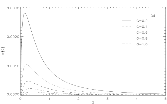
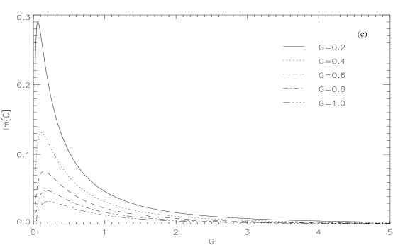
FIG. 2.: Imaginary part of $C$ for a logarithmic wind profile (a)$r=0.01$ (b)$r=0.1$ (c)$r=0.5$ .

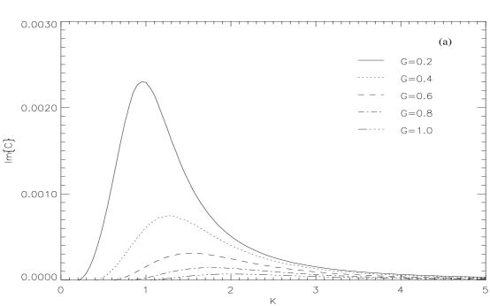
FIG. 3.: Imaginary part of $C$ for a tanh wind profile (a)$r=0.01$ (b)$r=0.1$ (c)$r=0.5$ .

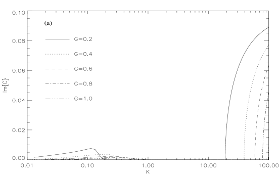
FIG. 4.: Imaginary part of $C$ for a logarithmic wind profile and $V_{o}$=1.0 (a)$r=0.01$, (b)$r=0.1$, (c)$r=0.5$ .

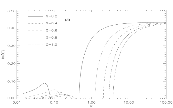
FIG. 5.: Imaginary part of $C$ for a logarithmic wind profile with $r=0.1$ and (a) $V_{o}$=0.0, (b)$V_{o}$=0.5, (c)$V_{o}$=1.0, (d) $V_{o}$=1.5 .

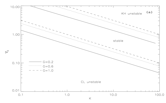
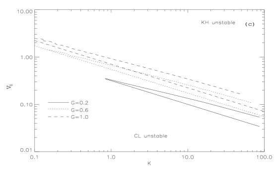
FIG. 6.: Stability boundaries for (a)$r=0.01$, (b)$r=0.1$, (c)$r=0.5$ .

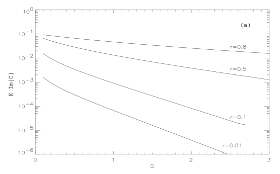
FIG. 7.: Growth rate of the fastest growing mode as a function of $G$ (a)logarithmic wind profile, (b) tanh wind profile .

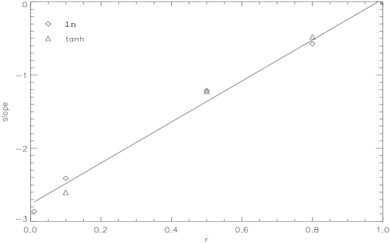
FIG. 8.: Slopes of the previous graph as a function of $r$ (e.g. the dependence of the exponent in eq. 33 on $r$).

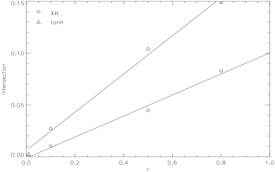
FIG. 9.: Intersections of the previous graph as a function of $r$ (e.g. the dependence of the coefficient in front the exponential in eq. 33, on $r$).

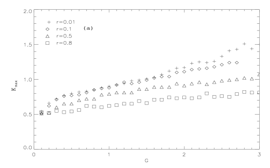
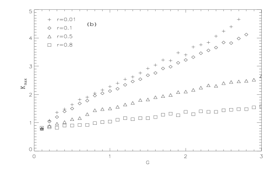
FIG. 10.: The dependence of the wavenumber of the fastest growing mode on $G$ (a)logarithmic wind profile, (b) tanh wind profile.

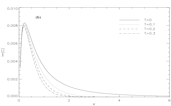
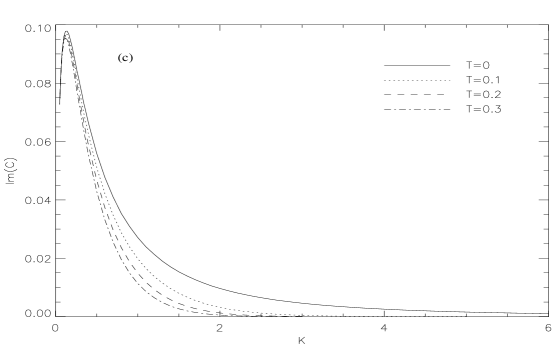
FIG. 11.: Imaginary part of $C$ for a logarithmic wind profile with G=0.5 in the presence of surface tension (a)$r=0.01$, (b)$r=0.1$, (c)$r=0.5$ .

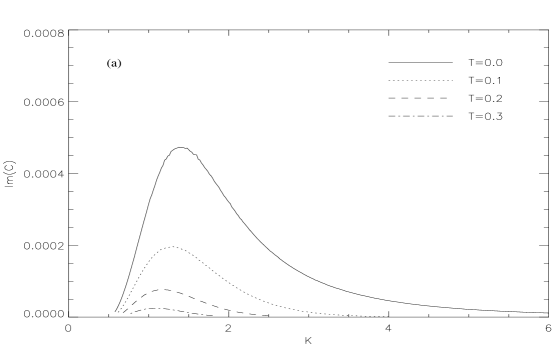
FIG. 12.: Imaginary part of $C$ for a tanh wind profile with G=0.5 in the presence of surface tension (a)$r=0.01$, (b)$r=0.1$, (c)$r=0.5$ .

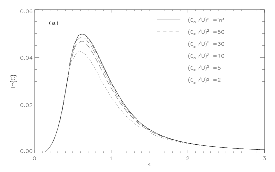
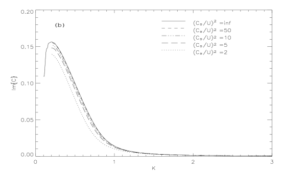
FIG. 13.: Im{$C$} for $r$=0.1 for the compressible case (a)$G$=0.1, (b)$G$=0.01 .

TABLE I.: Approximate range for parameter $G$ in three different situations.

	$\mbox{\rm U}_{1}$(cm s-1)	$g$ cm s-2	$a^{-1}$cm	G
ocean	$10^{2}\sim 10^{3}$	$10^{3}$	$10\sim 10^{2}$	$10^{-1}\sim 1$
Sun’s surface	$10^{2}\sim 10^{5}$	$10^{4.3}$	$10^{6}\sim 10^{7}$	$10^{1.3}\sim 10^{6.3}$
WD	$10^{4}\sim 10^{7}$	$10^{8}$	$10^{3}\sim 10^{6}$	$1\sim 10$

REFERENCES

- [1] Basset G.M. & Woodward P.R. 1995 Ap. J. 441,582 .
- [2] Bodo, G. & Massaglia, S. & Rossi P. & Rosner R. & Malagoli A. & Ferrari, A. 1995, A & A, 303,281 .
- [3] Chandrasekhar, S. 1962, Hydrodynamics (New York: Dover).
- [4] Chen, G., Kharif, C., Zaleski, S., & Li, J. 1999, Phys. Fluids, 11, 121.
- [5] Chimonas, G. 1970, JFM 43, 833
- [6] Cox J.P., & Giuli T.R. 1968,Stellar structure (Vol.182), (NY:Gordon& Breach)
- [7] Davis, P.A., & Peltier, W.R. 1976, J. Atmospheric Sci., 33, 1287.
- [8] Drazin, P.G. & Reid, W.H. 1981, Hydrodynamic Stability (Cambidge University Press).
- [9] Fujimoto, M.Y. 1982, ApJ, 257, 752.
- [10] Glasner, S.A., & Livne, E. 1995, ApJ, 445, L149.
- [11] Glasner, S.A., Livne, E., Truran, J.W. 1997, ApJ, 475, 754.
- [12] Hardee P.E., Norman M.L. 1988. Ap. J. 334,70 .
- [13] Howard, L.N. 1961, JFM, 10, 509.
- [14] Kercek, A., Hillebrandt, W., & Truran, J.W. 1998a, A& A, 337, 379.
- [15] Kercek, A., Hillebrandt, W., & Truran, J.W. 1998b, in Proc. Workshop on Fluid Dynamics, Bordaux, France, p. 14.
- [16] Kercek, A., Hillebrandt, W., & Truran, J.W. 1999, A& A,345, 831.
- [17] Kippenhahn, R., & Thomas, H.-C., 1978, A& A,63, 265.
- [18] Lighthill, M.J. 1962, JFM, 14, 385.
- [19] Lin, C.C. 1955, The Theory of Hydrodynamic Stability (Cambridge University Press).
- [20] Miles, J. 1957, JFM, 3, 185.
- [21] Miles, J. 1959a, JFM, 6, 568.
- [22] Miles, J. 1959b, JFM, 6, 583.
- [23] Miles, J. 1962, JFM, 13, 433.
- [24] Miles, J. 1967, JFM, 30, 163.
- [25] Miles, J. 1993, JFM, 256, 427.
- [26] Miles, J., & Ierley, G. 1998, JFM, 357, 21.
- [27] Rosner, R., Alexakis, A., Young, Y.N., Truran, J.W., & Hillebrandt, W. 2001, ApJL, to be submitted.
- [28] Rosner, R., Young, Y.N., Alexakis, A., Dursi, L.J., Truran, J.W., Calder, A.C., Fryxell, B., Olson, K., Ricker, PlM., Timmes, F.X., Zingale, M., & MacNeice, P. 2000, BAAS, 197, 81.06.
- [29] Shankar, A., & Arnett, W.D. 1994, ApJ, 433, 216.
- [30] Shankar, A., Arnett, W.D., & Fryxell, B.A. 1992, ApJ, 394, L13.
- [31] Starrfield, S., Sparks, W.M., & Truran, J.W. 1974, ApJS, 28, 247.
- [32] Starrfield, S., Truran, J., & Sparks, W.M. 1978, ApJ, 226, 186.
- [33] Starrfield, S., Truran, J., Sparks, W.M., & Kutter, G.G. 1978, ApJ, 176, 169.
- [34] Wallace, R.K., & Woosley, S.E. 1981, ApJS, 45, 389.
- [35] Woosley, S.E. 1986, in Nucleosynthesis and Chemical Evolution, eds. B. Hauck, A. Maeder, & G. Magnet (Sauverny: Geneva Observatory).
- [36] Young, Y.N., Alexakis, A., & Rosner, R. 2001, in preparation.