Tomographic Separation of Composite Spectra. VIII.
The Physical Properties of the Massive Compact Binary in the Triple Star System HD 36486 ($\delta$ Orionis A)

Abstract

We present the first double-lined spectroscopic orbital elements for the central binary in the massive triple, $\delta$ Orionis A. The solutions are based on fits of cross-correlation functions of IUE high dispersion UV spectra and He I $\lambda 6678$ profiles. The orbital elements for the primary agree well with previous results, and in particular, we confirm the apsidal advance with a period of $224.5\pm 4.5{\rm~{}y}$. We also present tomographic reconstructions of the primary and secondary stars’ spectra that confirm the O9.5 II classification of the primary and indicate a B0.5 III type for the secondary. The relative line strengths between the reconstructed spectra suggest magnitude differences of $\Delta m=-2.5\log(F_{s}/F_{p})=2.6\pm 0.2$ in the UV and $\Delta m=2.5\pm 0.3$ at 6678 Å. The widths of the UV cross-correlation functions are used to estimate the projected rotational velocities, $V\sin i=157\pm 6{\rm~{}km~{}s}^{-1}$ and $138\pm 16{\rm~{}km~{}s}^{-1}$ for the primary and secondary, respectively (which implies that the secondary rotates faster than the orbital motion).

We used the spectroscopic results to make a constrained fit of the Hipparcos light curve of this eclipsing binary, and the model fits limit the inclination to the range $i=67^{\circ}-77^{\circ}$. The lower limit corresponds to a near Roche-filling configuration that has an absolute magnitude which is consistent with the photometrically determined distance to Ori OB1b, the Orion Belt cluster in which $\delta$ Ori resides. The $i=67^{\circ}$ solution results in masses of $M_{p}=11.2~{}M_{\odot}$ and $M_{s}=5.6~{}M_{\odot}$, both of which are substantially below the expected masses for stars of their luminosity. The binary may have experienced a mass ratio reversal caused by Case A Roche lobe overflow, or the system may have suffered extensive mass loss through a binary interaction (perhaps during a common envelope phase) in which most of the primary’s mass was lost from the system rather than transferred to the secondary.

We also made three component reconstructions to search for the presumed stationary spectrum of the close visual companion, $\delta$ Ori Ab (Hei 42 Ab). There is no indication of the spectral lines of this tertiary in the UV spectrum, but a broad and shallow feature is apparent in the reconstruction of He I $\lambda 6678$ indicative of an early B-type star. The tertiary may be a rapid rotator ($V\sin i\approx 300{\rm~{}km~{}s}^{-1}$) or a spectroscopic binary.

1 Introduction

In this series of papers we have applied a version of the Doppler tomography algorithm (Bagnuolo et al., 1994) to reconstruct the component ultraviolet and optical spectra of massive close binary systems, and we have investigated their spectral morphology, rotational velocities, and relative flux contributions. We were successful in three component spectral reconstructions of the triple systems 55 UMa (Liu et al., 1997) and $\delta$ Cir (Penny et al., 2001), and we are continuing to examine the ultraviolet spectra of several OB systems known to be triples from speckle interferometry (Mason et al., 1998). Here we turn our attention to the most famous of this group, and one of the brightest O-stars in the sky, $\delta$ Orionis.

The visual and spectroscopic components of the $\delta$ Orionis system (Mintaka, 34 Ori, HD 36486, HR 1852, BD–00 983, ADS 4134, Hei 42, HIP 25930) are depicted in Fig 1. The Washington Double Star Catalog (Worley & Douglass, 1997) lists two distant visual companions: $\delta$ Ori B (BD–00 983B), a 14.0 mag star 33$\arcsec$ away, and $\delta$ Ori C (HD 36485), a 6.85 mag star at a separation of 53$\arcsec$. Both of these targets are far outside the spectroscopic apertures used on the International Ultraviolet Explorer Satellite (IUE), and so will not be considered further here. However, the remaining visual companion, $\delta$ Ori Ab (Hei 42 Ab), is very close, and its light will contribute to the spectra we discuss below. This companion was discovered by Heintz (1980) in 1978 at a separation of $0\farcs 2$, and subsequent speckle interferometry (McAlister & Hendry, 1982; McAlister et al., 1983, 1987, 1989, 1993; Hartkopf et al., 1993; Mason et al., 1998; Prieur et al., 2001) indicates a linear motion widening by 5.7 mas y^-1. The Hipparcos satellite found this companion at a separation of $0\farcs 267\pm 0\farcs 003$ in 1993 and determined a magnitude difference between the Aa and Ab components of $\Delta H_{p}=1.35\pm 0.03$ mag (Perryman, 1997).

The bright central object, $\delta$ Ori A (O9.5 II, Walborn (1972)), is a single-lined spectroscopic binary with a period of $5\fd 7325$ (Harvey et al., 1987). Orbital solutions exist which span the last century (Hartmann, 1904; Jordan, 1914; Curtiss, 1914; Hnatek, 1920; Luyten et al., 1939; Pismis et al., 1950; Miczaika, 1952; Natarajan & Rajamohan, 1971; Singh, 1982), and these are summarized by Harvey et al. (1987) who present the most recent solution based upon 44 high dispersion spectra from IUE. In addition, Harvey et al. (1987) reanalyzed all the published data and found convincing evidence of a regular advance in the longitude of periastron, giving an apsidal period of $225\pm 27$ y.

Spectroscopic investigations to date have failed to identify clearly the secondary and tertiary (Hei 42 Ab) spectral components in the composite spectrum. The first detection of the secondary was claimed by Luyten et al. (1939) who observed its orbital motion in weak extensions of He I $\lambda 4471$ in 6 of their 140 photographic spectra (with a semiamplitude ratio of $K_{2}/K_{1}=2.6$). Galkina (1976) reported evidence of the secondary star’s contribution in the He I $\lambda 5876$ profile, and found the antiphase motion amounting to $K_{2}/K_{1}=1.6-1.7$. Galkina (1976) estimated a spectral type of B1 for the secondary and a magnitude difference of $\Delta m=2.0-2.5$ mag in the optical region.

The central binary also exhibits partial eclipses, and Koch & Hrivnak (1981) have analyzed both their photometric observations and the available, historical light curves. The analysis is made difficult by the presence of intrinsic light variability in one or more of the components and the presence of third light. Nevertheless, Koch & Hrivnak (1981) were able to make a reasonable fit of the light curve by assuming a detached (but near Roche-filling) configuration. Their best fit model led to a primary of $23~{}M_{\sun}$, $17~{}R_{\sun}$, and $T_{\rm eff}=31100$ K, a secondary of $9~{}M_{\sun}$, $10~{}R_{\sun}$, and $T_{\rm eff}=25000$ K, an optical magnitude difference $\Delta m=1.4$ mag, and an orbital inclination of about $i=68^{\circ}$. However, Koch & Hrivnak (1981) had to rely on Heintz’s visual report of a third light magnitude difference of $\Delta m=0.1$ mag, implying a much brighter Ab component than found by Hipparcos ($\Delta m=1.35$ mag), and this suggests that their corrected eclipse depths are too deep.

In this paper we present our own analysis of the 60 available IUE high-dispersion SWP spectra of $\delta$ Ori A plus a set of spectra of the He I $\lambda 6678$ line. In the next section (§2), we describe the IUE observations and our cross-correlation methods for radial velocity measurement. The optical spectra and radial velocity measurements are presented in §3. A new double-lined orbit is given in §4 along with a discussion of the apsidal motion and long term changes in systemic velocity. Next (§5), we use Doppler tomography to separate the individual component spectra, which are then examined to obtain MK classifications, projected rotational velocities, and relative flux contributions. We analyze the Hipparcos light curve in §6, and discuss in §7 the evolutionary implications of the resulting masses and other parameters.

2 IUE Observations and Radial Velocities

There are 60 high-dispersion, short wavelength prime (SWP) camera spectra of $\delta$ Ori A available in the IUE Final Archive at the Space Telescope Science Institute’s Multi-mission Archive. These spectra have a signal-to-noise ratio (S/N) of approximately 10 per pixel. They were made with both the large and small apertures. They were retrieved in NEWSIPS format (Garhart et al., 1997). A log of observations, including the SWP image number and the heliocentric time of mid-observation appears in Table 1.

Once we retrieved the spectra, they were processed using local procedures written in IDL that assemble the spectra into an array of dimensions of wavelength and time. During this process, the spectra are smoothed from the nominal 30  km s^-1 FWHM resolution of the raw spectra to 40  km s^-1 FWHM. The spectra are rectified using a set of relatively line-free zones, and resampled using a uniform log $\lambda$ wavelength grid (in increments equivalent to $10{\rm~{}km~{}s}^{-1}$). The major interstellar lines are used to co-align the spectra on a common velocity frame, and then these lines are replaced by straight-line segments. Details are given in Penny et al. (1997).

We then cross-correlated the spectra with the spectrum of a narrow-lined reference template star, AE Aurigae (HD 34078; O9.5 V; $V\sin i=30{\rm~{}km~{}s}^{-1}$; $V_{r}=+54.4{\rm~{}km~{}s}^{-1}$, Gies & Bolton (1986)). The template was produced from an average of 6 SWP spectra of AE Aur prepared using the same methods that we used to produce the $\delta$ Ori matrix of spectra. The cross-correlation was performed over the velocity range $-1000$ to $+1000{\rm~{}km~{}s}^{-1}$ relative to the reference star to produce a matrix of cross-correlation functions (the composite ccfs) of dimensions relative velocity and time. The regions around the broad features of Ly$\alpha$, Si IV $\lambda 1400$, and C IV $\lambda 1550$ were set to unit intensity (featureless continuum) before cross-correlation to insure that the resulting ccfs have shapes similar to the rotationally broadened photospheric lines. Finally the ccfs were rectified by division of a straight line fit made of the extreme ends of the ccfs. This step makes possible the direct comparison of ccfs made from spectra of varying quality (S/N ratio), but we caution that in this representation the ccf central depths may vary depending on spectrum quality.

The final ccfs are presented in Figure 2 as a function of absolute radial velocity and orbital phase. The orbital motion of the primary star (Aa1) is clearly evident in the varying position of the central minimum and accompanying broad wings of the ccfs (termed “pedestal” by Howarth et al. (1997)). There is no obvious indication of a secondary (or a stationary tertiary) component, but we demonstrate below that the shapes of the ccfs are indeed influenced by the moving secondary component.

We first attempted to measure radial velocities for the primary component by fitting a parabola through the 5 points (spanning $50{\rm~{}km~{}s}^{-1}$) surrounding the ccf minimum. This procedure proved unsatisfactory because the residuals from the fit were rather large (due to fitting only a small portion of the ccf) and because inspection of the quadrature phase ccfs showed asymmetrical extensions indicating the presence of a partially blended, weak secondary component. Our solution to the fitting problem involved determining an empirical shape for the ccf component of the primary and a constrained Gaussian function for the secondary, and these components were then fit in a least-squares model to determine the positions (and hence radial velocity shifts) for each component. The following paragraphs describe the details of the fitting procedure. Our final measurements are listed in Table 1, and are discussed below (§4).

The ccfs are dominated by the central core and broad wings of the primary component, and our first task was to isolate the functional shape of this component. During orbital phases when the primary is significantly blue-shifted, the short wavelength half of the profile is mainly clear of the blending influence of the secondary (or a possible stationary third component) while the long wavelength side is free of blending at the opposite red-shifted phases. We therefore formed two versions of the primary component’s profile by using a shift-and-add algorithm and our preliminary orbital solution to obtain the mean profile near the times of each quadrature. These two means were then averaged using window functions of the form $(1+e^{x})^{-1}$ (with $x=\triangle V_{r}/50~{}{\rm~{}km~{}s}^{-1}$) for the blue-shifted mean and $(1+e^{-x})^{-1}$ for the red-shifted mean, to obtain a final primary reference ccf which varied smoothly through the line core (illustrated in Fig. 3).

The next step was to define a functional shape for the secondary component in the ccf. This was done by fitting the primary reference ccf to the best resolved quadrature phase ccfs over the range from the ccf minimum to the high velocity wing in the direction away from the secondary. This fit was then subtracted away, and the residual ccf due to the secondary alone was fit with an unconstrained Gaussian profile. There were no obvious differences between the derived Gaussian widths or depths of the fits from the two quadratures, so we averaged all the Gaussian fit parameters to arrive at a mean standard deviation width, $\sigma=(89\pm 8){\rm~{}km~{}s}^{-1}$, and ratio of central depth to primary reference ccf depth of $0.09\pm 0.02$. We adopted these parameters to fix the shape of the secondary ccf component.

The final step was to fit the sum of these profiles to each individual ccf. This was accomplished using a non-linear, least-squares fitting of the primary and secondary functional curves based upon three parameters, the primary and secondary radial velocities and a normalization factor for overall ccf depth (to account for varying quality of the input spectra). An example of the detailed fitting procedure is illustrated in Figure 3 which shows the model primary and secondary functions and how their sum gives excellent agreement with the observed ccf (for a phase near primary velocity maximum). This plot demonstrates the importance of defining the shape of the primary component wings in order to place correctly the secondary component. The residuals formed after removal of only the primary component in these fits are shown in Figure 4. This plot shows that although the secondary component is weak, it is nevertheless found in most of the ccfs, moves with the expected period, and is antiphase to the primary’s orbit. The average ccf variance per pixel in the inner $\pm 200$ km s^-1 of the velocity range in Figure 4, the range that bounds the secondary’s Doppler shifts, is 1.5% (or about one sixth of the height of the scale bar illustrated) based upon differences in ccfs from multiple spectra obtained sequentially. This is $\approx 67\%$ of the the secondary’s depth in the residual ccfs, so the secondary’s ccf contribution is slightly greater than the noise level in individual pixels. The final velocity measurements on the absolute scale are listed in Table 1, and the radial velocity curves are illustrated in Figure 5.

These results indicate that the secondary’s contribution to the composite ccf is always weak and partially blended with the primary’s ccf component. It is therefore important to review the limitations of our methods and the possible systematic errors that may be present in these difficult measurements. The first shortcoming is that there probably exists an additional stationary component in the composite ccfs that is not included in our simple two-component model. The grayscale portion of Figure 4, for example, indicates that there is a very weak, narrow, and stationary feature in the residuals near a radial velocity of $+54{\rm~{}km~{}s}^{-1}$ which we suggest results from a correlation between unexcised interstellar lines in the spectrum of $\delta$ Ori with their counterparts in the AE Aur photospheric spectrum (since this velocity corresponds to the radial velocity of AE Aur). It is also possible that there is a weak, stationary ccf component near the systemic velocity due to the tertiary (although there is no evidence of this in Fig. 4 nor from tomographic experiments described below). Any such stationary feature would tend to pull the two-component fits back towards the stationary component, so that the velocity excursions would be underestimated in our measurements. We did a numerical experiment to estimate the size of this error by artificially removing from the composite ccfs a stationary component to represent a possible tertiary contribution. We assumed that the third component had a shape like the primary’s reference ccf but was reduced to 10% of the primary’s central depth and centered at the systemic velocity. We then repeated the measurement process by forming a primary reference profile from the quadrature phase ccfs, fitting a Gaussian to the isolated secondary component, and then fitting all the adjusted ccfs for the positions of primary and secondary. These fits were generally less satisfactory and we do not list the individual velocities here, but the orbital elements based upon this experiment are given in the fourth column of Table 3 under the heading “Adjusted UV ccfs”. A comparison with our nominal set of elements (third column of Table 3) shows that the semiamplitudes may be underestimated (by $\approx$ 8% for $K_{1}$ and 14% for $K_{2}$ in this particular case) if such a third component is present. This effect, if fully present in both components, could raise our estimated masses by 43% (§6).

A second area of concern is the parameterization of the secondary component’s width and depth. Our choices for these parameters appear to be supported by observations of the optical line He I $\lambda 6678$ (§3), but the results are sensitive to the values of these parameters. If the secondary profile is set to be wider and/or deeper, then the observed ccfs are fit with smaller radial velocity excursions. For example, we made a test with a secondary Gaussian component with a mean standard deviation, $\sigma=128{\rm~{}km~{}s}^{-1}$, and a ratio of central depth to primary reference ccf depth of $0.10$, and the resulting measurements led to a secondary semiamplitude of $K_{2}=112{\rm~{}km~{}s}^{-1}$ which is much smaller than our nominal (preferred) value of $K_{2}=186{\rm~{}km~{}s}^{-1}$. Finally, the reader should be aware of potential problems resulting from our assumption that the component ratios and functional shapes are constant with orbital phase. At the conjunction phases for example, the partial eclipses will change the relative contributions of the primary and secondary components so that our fixed ccf depth ratio may lead to systematic errors in the velocity placement. Furthermore, the photometric light curve indicates that the primary is close to Roche filling (Koch & Hrivnak, 1981), and consequently we expect that the primary’s photospheric lines will show subtle width variations, appearing slightly narrower (wider or asymmetric) at conjunctions (quadratures). However, a comparison of our primary reference ccf (which was formed from the quadrature ccfs) with conjunction phase ccfs indicates only minor differences so we doubt that our radial velocity measurements are badly in error at conjunctions.

3 Radial Velocities from He I $\lambda 6678$

The binary was also observed in the optical by Thaller (1997a) in a program to search for incipient H$\alpha$ emission from colliding winds. Thaller (1997b) found that H$\alpha$ is sometimes distorted by residual emission effects, but He I $\lambda 6678$ is relatively free of emission problems most of the time. There are 20 spectra in this set which were obtained with the Kitt Peak National Observatory Coude Feed Telescope and the Mount Stromlo Observatory 74-inch Telescope (Thaller, 1997a), and these spectra generally have better resolution ($\lambda/\Delta\lambda=14000-32000$) and S/N ratio ($\approx 200-300$ pixel^-1) than the IUE ccfs discussed above. The He I $\lambda 6678$ profiles are illustrated as a function of orbital phase in Figure 6. There appears to be a weak extension present at both quadratures that is probably the signature of the secondary (although part of the red wing depression is due to a weak He II $\lambda 6683$ feature in the primary’s spectrum).

The He I $\lambda 6678$ profiles were fit in the same way as the UV ccfs by forming a mean quadrature profile for the primary and fitting the residual secondary component with a Gaussian with a mean standard deviation, $\sigma=(86\pm 20){\rm~{}km~{}s}^{-1}$ and ratio of central depth to primary depth of $0.10\pm 0.02$ (both of these parameters are identical within errors with those found from the UV ccfs). The fits were generally good, and we show in Figure 7 the residuals after the removal of the fitted primary component alone. The motion of the secondary component is clearly seen in these residuals. The radial velocities from the two-component fit are listed in Table 2 and plotted in Figure 8. Note that we zero weighted three sets of measurements in the orbital solutions below that corresponded to profiles which were visibly contaminated with the emission pattern seen in H$\alpha$.

4 Orbital Elements

We solved for the orbital elements using the non-linear, least-squares fitting program described by Morbey & Brosterhus (1974). The fit progressed in several steps. First, we fit the UV ccf radial velocities of the primary component by solving for all six orbital elements. Since the radial velocity measurements of the secondary generally have larger errors, we then fixed the values of the period, $P$, epoch of periastron, $T$, eccentricity, $e$, and longitude of periastron, $\omega$, to those from the primary’s solution, and solved only for the secondary systemic radial velocity, $\gamma$, and semiamplitude, $K$. In Table 3, we compare the results from the UV ccf velocities (column 3) with those of Harvey et al. (1987) (column 2). This table also lists the elements resulting from a numerical experiment (§2) which shows the influence of a potentially unaccounted for tertiary component in our fitting of the UV ccfs (column 4). We have relatively fewer radial velocities from fits of the He I $\lambda 6678$ profile, and so we fixed the period and eccentricity at the values from the UV ccf solution in fitting the He I $\lambda 6678$ data (column 5). The computed radial velocity curves are plotted in Figures 2 and 4 – 8.

Our results (with the exception of $\omega$ and $\gamma$; see below) are generally in good agreement with the single-lined spectroscopic orbital solution found by Harvey et al. (1987), and our formal errors are similar to or smaller than theirs. We give in Table 3 the mean sidereal period rather than the anomalistic period given by Harvey et al. (1987). Our derived period agrees with theirs within errors, although we find somewhat better agreement with the photometric period of 5.732476 d adopted by Koch & Hrivnak (1981).

The largest errors are associated with the secondary semiamplitude, $K_{2}$, which unfortunately propagates into a large error in the quantity $m_{1}\sin^{3}i$. The root-mean-square (rms) residuals are smaller for the secondary radial velocity measurements from the higher quality He I $\lambda 6678$ profiles. Our value of $K_{2}$ is much smaller than first claimed by Luyten et al. (1939) but is slightly larger than that found by Galkina (1976). Given the faintness and line blending problems associated with the secondary’s lines, this kind of disagreement is not surprising.

The greatest difference between our results and prior work is the evident increase in longitude of periastron, $\omega_{1}$, due to apsidal motion. Harvey et al. (1987) performed a comprehensive non-linear, least squares analysis of the entire body of 546 historical and new velocities using $\dot{\omega}_{1}$ as a free parameter and fixing the systemic velocity at $+20.3{\rm~{}km~{}s}^{-1}$. They found an apsidal motion of $(1.60\pm 0.20)$ ^∘ y^-1, giving a period of $225\pm 27$ y, in excellent agreement with an earlier comprehensive result of $227\pm 37$ y from Monet (1980). We have added our results from the expanded IUE ccf and He I $\lambda 6678$ solutions to the historical derivations of $\omega_{1}$ given in Harvey et al. (1987), and the entire set is plotted as a function of time in Figure 9. The error weighted, linear fit is also shown which yields the same rate for the apsidal advance as found by Harvey et al. (1987), $(1.60~{}\pm~{}0.03)~{}^{\circ}$ y^-1, giving an apsidal period of $224.5\pm 4.5$ y. Note that apsidal advance in $\delta$ Ori may result from both the tidal forces between the two components of the close binary and the influence of the orbiting third body.

It is possible that the reflex motion of the central binary in its orbit about the center of mass of the binary-tertiary system might produce measurable, long-term variations in the systemic velocity of the central binary. We show in Figure 10 estimates of the systemic velocity from solutions based on data spanning the last century (Harvey et al., 1987) plus our own estimates from Table 3. There is a suggestion in this plot of a real variation in which the systemic velocity reached a minimum around 1940 and is currently increasing. The IUE solution corresponds to the highest point in this graph, and we caution that the apparent discrepancy may be due in part to systematic differences between radial velocities for the lines in the UV and optical. Hutchings (1976) demonstrated that velocity progressions exist in hot, luminous stars between lines formed deep in the photosphere and those of lower excitation formed higher in the atmosphere where acceleration into the stellar wind is occurring. Many of the strong optical lines (the Balmer series and He I lines) probably reflect the outflow as a negative radial velocity offset compared to the higher excitation lines measured in the UV ccfs (formed at higher temperature deeper in the photosphere), and thus, the systemic velocity from the optical studies would be lower than that from our IUE solution. We note that Hutchings (1976) found no measurable velocity – excitation correlation in his optical spectra of $\delta$ Ori, but a difference of $10{\rm~{}km~{}s}^{-1}$ between the radial velocities of the low and high excitation lines is smaller than his threshold for detection.

5 Tomographic Reconstruction of the Individual Spectra

We used an iterative Doppler tomography algorithm (Bagnuolo et al., 1994) to reconstruct the spectra of the individual component stars in the $\delta$ Orionis A system. The algorithm assumes that each observed composite spectrum is a linear combination of spectral components with known radial velocity curves (Table 3) and flux ratios that are constant across the spectral range and throughout the orbital cycle. The latter condition is violated by the partial eclipses that occur at conjunctions (§5), but since the eclipses are shallow and only a minority of our spectra were obtained during eclipse phases, flux constancy is a reasonable assumption. We estimated the UV flux ratio, $F_{s}/F_{p}(UV)=0.095\pm 0.021$, from the ratio of the areas of Gaussian fits of the UV ccf reference profiles. Note that the actual error is probably larger than quoted since we have not accounted for changes in the ccf amplitude related to differences in the match of the ccf template spectrum of AE Aur to the slightly different spectral patterns of the primary and secondary. Likewise, we estimated the optical band flux ratio as $F_{s}/F_{p}(opt)=0.097\pm 0.027$ based upon the ratio of the He I $\lambda 6678$ reference component equivalent widths. Again, this estimation does not account for differences in equivalent width of He I $\lambda 6678$ between the spectral types of the primary and secondary. We took the Hipparcos magnitude difference for the tertiary to estimate its optical flux ratio as $F_{t}/(F_{p}+F_{s})(opt)=0.288\pm 0.009$. Note that the tertiary is actually the second brightest star of the three in the visual region. We do not know the UV flux contribution of the tertiary, so we produced UV reconstructions assuming both zero flux and the optical flux ratio.

The reconstructed spectra in the vicinity of He I $\lambda 6678$ are illustrated in Figure 11. The primary and secondary components both have a strong He I $\lambda 6678$ feature, and He II $\lambda 6683$ is also visible in the red wing of the primary’s profile. The tertiary, on the other hand, has a very shallow and broad He I $\lambda 6678$ feature which is shifted redward by $27{\rm~{}km~{}s}^{-1}$ compared to the systemic velocity of the central binary. The equivalent width of the profile in the tertiary reconstruction is comparable to those of the primary and secondary, and this suggests that the tertiary has an early B-type classification. The extreme width of the reconstructed tertiary profile indicates that either it is a rapid rotator ($V\sin i\approx 300{\rm~{}km~{}s}^{-1}$) or that it is a spectroscopic binary with a radial velocity range similar to the line width in the reconstruction.

A portion of reconstructed UV spectrum of the primary appears in Figure 12, and the S/N in the reconstructed spectrum is excellent thanks to the large number of spectra used in the reconstruction. Penny et al. (1997) developed a system of spectral classification in the UV based upon the equivalent widths of a set of prominent photospheric spectral lines that are sensitive to temperature and luminosity. We used this method with the reconstructed primary spectrum to derive a classification of O9.5 III based on the two component reconstruction or B0 I based on the three component reconstruction (in which the primary has deeper lines) using the following criteria: the equivalent widths of Si III $\lambda 1299$, Fe V $\lambda 1429$, He II $\lambda 1640$, Fe IV $\lambda 1681$, Fe IV $\lambda 1765$, and the line ratios of He II $\lambda 1640$/Fe V $\lambda 1429$ and Fe IV $\lambda 1723$/Fe V $\lambda 1429$. The luminosity class is set by the equivalent width of N IV $\lambda 1718$ which is used to assign a class of I, III, or V. These UV-based criteria are fully consistent with the optical classification of O9.5 II (Walborn, 1972).

The depths of the lines in the reconstructed spectrum of the primary offer a means to check on our assumed flux contribution of the tertiary. If we assigned too much flux to the tertiary, for example, then the primary’s lines will appear too deep in the reconstructed spectrum. We can test this possibility through a direct comparison of the reconstructed spectrum with that of a single star of the same spectral classification and rotational broadening. We selected 19 Cep (HD 209975) for this purpose which has a similar classification (O9.5 Ib) but slightly narrower lines ($V\sin i=90{\rm~{}km~{}s}^{-1}$; Penny (1996)). We used the reference ccf widths to estimate the projected rotational velocities using the method of Penny (1996) to arrive at $V\sin i=157\pm 6{\rm~{}km~{}s}^{-1}$ and $138\pm 16{\rm~{}km~{}s}^{-1}$ for the primary and secondary, respectively. Then we artificially broadened the spectrum of 19 Cep to match the line broadening of the primary. The resulting spectrum of 19 Cep (dotted line) is compared to that of the primary in Figure 12 for the cases where the tertiary contributes no UV flux (thick solid line) and where it contributes the fraction measured in the optical (thin solid line). Taken at face value, this comparison indicates that the tertiary contributes little if any UV flux.

The reconstructed secondary spectrum is noisy because of the star’s relative faintness, and this reconstruction is also marred by the effects of incomplete removal of the echelle blaze function (“ripple”) in the reduction software (Fig. 13). Furthermore, several features useful for spectral classification in B-type stars were excised during the process of interstellar line removal (e.g., Si II $\lambda 1265$, C II $\lambda\lambda 1334,1336$). Nevertheless, a number of prominent spectral features are discernible and indicative of an early-B spectral type. Since the classification scheme of Penny et al. (1997) is valid only for O-type stars, we relied instead on the classification criteria described by Rountree & Sonneborn (1993) and Massa (1989). Massa (1989) found that the equivalent width of Si III $\lambda 1417$ is luminosity sensitive in early-B stars, and the measured value in the secondary, $\log W_{\lambda}($mÅ$)=2.49\pm 0.04$ indicates luminosity class III which is consistent with the observed strength of other luminosity sensitive lines discussed by Rountree & Sonneborn (1993). Based upon a comparison of the relative line strengths in the spectra of giants presented in Rountree & Sonneborn (1993), the spectral type falls in the range B0–B1 using C III $\lambda 1247$, B1–B3 using Si III $\lambda 1299$, B0.5–B1 using He II $\lambda 1640$, B0–B0.5 using N IV $\lambda 1718$, and B0.5–B1 using N III $\lambda\lambda 1748,1751$. Thus, the secondary has a UV spectrum consistent with a B0.5 III classification. The secondary spectrum is compared in Figure 13 to the co-added spectrum of a similar star, $\epsilon$ Per (B0.5 IV-III, $V\sin i=134{\rm~{}km~{}s}^{-1}$; Tarasov et al. (1995); Gies et al. (1999)). The reconstructed secondary does exhibit P Cygni type profiles of N V $\lambda 1240$, Si IV $\lambda 1400$, and C IV $\lambda 1550$ indicative of an earlier or more luminous star, but we caution that the tomographic reconstructions are problematical in the immediate vicinity of these lines which often lack obvious orbital motion (Gies, 1995). Our B0.5 III classification is consistent with the optical detections of the secondary’s lines in He I $\lambda 4471$ (Luyten et al., 1939), He I $\lambda 5876$ (Galkina, 1976; Fullerton, 1990), and in our tomographic reconstruction of He I $\lambda 6678$ (Fig. 11).

In spite of the fact that our algorithm has successfully detected tertiary components in the cases of $\delta$ Cir (Penny et al., 2001) and 55 UMa (Liu et al., 1997), the reconstruction of the UV spectrum of the tertiary (made assuming it was stationary over the time span of the IUE observations) is essentially featureless, so that its UV spectral features remain undetected. We show in Figure 14 a portion of this spectrum plotted with that of the rapid rotator, $\zeta$ Oph (O9.5 V, $V\sin i=400{\rm~{}km~{}s}^{-1}$; Reid et al. (1993)). This comparison spectrum demonstrates how rapid rotation causes most features to become blended into a pseudo-continuum, so that a rapidly rotating tertiary would be difficult to detect in the reconstruction. However, this comparison also shows that certain strong features (such as N IV $\lambda 1718$) should still be relatively deep in the UV spectra of rapid rotators, and their absence in the tertiary spectrum reinforces the impression derived from the depths of the primary’s lines that the tertiary contributes only a minor fraction of the UV flux (certainly less than it does in the optical). Such a low UV flux contribution is puzzling given the relative brightness of the tertiary in the optical and the indication from the He I $\lambda 6678$ reconstruction that it is a B-type star. On the other hand, the lack of features in the tertiary spectrum suggests that the radial velocities derived from our two component fits of the UV ccfs should be relatively free of systematic errors due to line blending with the tertiary spectrum (so that the trial orbital elements in column 4 of Table 3 based on a tertiary with lines 10% as deep as the primary’s represents an extreme and unlikely case).

6 Light Curve and Masses

Photometry from the Hipparcos Satellite (Perryman, 1997) provides a contemporary light curve for the central binary (Fig. 15), and although this light curve suffers from gaps in coverage and additional intrinsic variability (Koch & Hrivnak, 1981), we will compare it to model orbital variations to obtain preliminary limits on the system inclination, $i$ (and hence the masses). We used the light curve synthesis code GENSYN (Mochnacki & Doughty, 1972) to produce model $V$-band differential light curves (almost identical to differential Hipparcos magnitudes for hot stars). The code was written for binaries with circular orbits, and we used multiple runs to synthesize the varying orbital separation in an elliptical orbit (Penny et al., 1999). Our approach was to make a constrained fit using as much data as possible from our spectroscopic results. The orbital parameters were taken from the UV ccf solutions (using an interpolated longitude of periastron, $\omega=128^{\circ}$, for the average time of observation, BY 1991.2; see Fig. 9). The stellar temperatures and gravities were taken from Voels et al. (1989) for the primary ($T_{\rm eff}=33,000$ K and $\log g=3.4$), and for the secondary we used estimates from Tarasov et al. (1995) for a comparable star, $\epsilon$ Per ($T_{\rm eff}=27,600$ K and $\log g=3.8$). We then estimated the physical fluxes and limb darkening coefficients from tables in Kurucz (1994) and Wade & Rucinski (1985), respectively. The secondary’s polar radius was set at $0.37~{}R_{p}$ (where $R_{p}$ is the assumed primary’s polar radius) based upon our estimated magnitude difference, $\Delta V=2.5$ (§5), and the calculated surface fluxes. Finally, we set the rotational periods of the stars based upon the assumed values of $R_{p}$ and $i$ and the measured projected rotational velocities (§5). Each trial run of GENSYN was defined by two model parameters, $R_{p}$ and $i$, and all the resulting light curves were corrected for the presence of third light using the Hipparcos flux ratio, $F_{t}/(F_{s}+F_{p})=0.29$.

The Hipparcos light curve is illustrated in Figure 15 as a function of photometric phase based upon the predicted time of minimum light according to the ephemeris from the UV ccfs for the primary (Table 3). We also show two model light curves which provide only marginally satisfactory fits but which correspond to the probable limits of our fitting parameters. The solid line is the model light curve for $R_{p}/R_{\odot}=13$ and $i=67^{\circ}$ which represents the largest size primary consistent with the fitting scheme. The primary in this model has a polar radius only 1% smaller than the critical Roche radius at periastron. The Roche radius can be somewhat larger than $13~{}R_{\odot}$ in models with lower inclination (since the system dimensions are set by $a\sin i$), but Roche-filling models with lower inclination cannot produce eclipses as deep as those observed, so $i=67^{\circ}$ represents a reliable lower limit for the inclination. This is fortuitously close to the inclination adopted by Koch & Hrivnak (1981), $i=68^{\circ}$, since they adopted very different values for the mass ratio and third light correction. This near Roche-filling model is characterized by large ellipsoidal variations that shape the light curve outside of the eclipses. These appear to match the observations better in the photometric phase range 0.6 – 0.9 than in the range 0.2 – 0.4. In fact, the observations in the 0.2 – 0.4 range are better fit by a smaller, less tidally distorted model primary, and the dashed line indicates such a model for $R_{p}/R_{\odot}=9$ and $i=77^{\circ}$. This smaller primary model does a better job of matching the relative depths of the eclipses, but the duration of the eclipses may be too short especially when compared to the light curve observations of Koch & Hrivnak (1981). Thus, the inclination range $67^{\circ}-77^{\circ}$ appears to span the acceptable limits of plausible fits. This range corresponds to primary and secondary masses of $9.4-11.2~{}M_{\odot}$ and $4.8-5.6~{}M_{\odot}$, respectively (based upon the UV ccf orbital solutions).

7 Discussion

The IUE ccfs and He I $\lambda 6678$ line profiles have provided us with the first clear and consistent measurements of the orbital motion of the secondary star. However, the secondary’s resulting semiamplitude is surprisingly small, and consequently, our results indicate a binary with a smaller semimajor axis (implying lower masses) than expected. In particular, the mass of the primary is a factor of 3 to 4 below that predicted for a normal single star with its classification and stellar wind properties (Voels et al., 1989; Howarth & Prinja, 1989).

Such low mass results are not unprecedented. For additional examples of orbital masses that are significantly lower ($\approx$ 40%) than theoretical expectations, see the cases of LZ Cep (Harries et al., 1998) and $\delta$ Cir (Penny et al., 2001). In addition, Herrero et al. (1999, 2000) use model atmospheres to find masses for single O stars, and in some cases, they also find masses that are significantly lower than those expected from evolutionary tracks.

To attain a primary mass of $30M_{\odot}$ would require a 51% upward revision in the secondary’s semiamplitude, to $K_{2}=281{\rm~{}km~{}s}^{-1}$ (for $i=67^{\circ}$ and $K_{1}=94.9{\rm~{}km~{}s}^{-1}$), placing the secondary’s radial velocity range between $-230$ and $+330{\rm~{}km~{}s}^{-1}$. This would appear to be ruled out by the observed quadrature line profiles (see Figs. 4 and 7). Our derived value of $K_{2}$ (and the small masses implied) clearly requires additional verification (through high S/N and high dispersion spectroscopy of metal lines unaffected by emission, for example), but taken at face value, our results suggest that the current state of the primary is the result of extensive mass loss caused by an interaction with the secondary.

The absolute magnitudes of the components provide a reference point to assess the apparent mass - luminosity discrepancy of the components. The three bright Belt stars in Orion, $\delta$ Ori, $\epsilon$ Ori (B0 Ia), and $\zeta$ Ori (O9.7 Ib), form the high luminosity end of the Ori OB1b subgroup (Brown et al., 1994; de Zeeuw et al., 1999) which has an estimated age between 1.7 My (Brown et al., 1994) and 7 My (Blaauw, 1991). The distance to Ori OB1b is estimated to be $360\pm 70$ pc based on photometry (Brown et al., 1994) or $473\pm 33$ pc based on Hipparcos parallax measurements (de Zeeuw et al., 1999). Outside of eclipse, the apparent magnitude of $\delta$ Ori is $m_{V}=2.19$ (see Fig. 15 and the $H_{p}$ to $V$ transformation in Harmanec (1998)), which for an extinction of $A_{V}=0.16$ mag (Brown, 1996), gives the absolute magnitude of the triple as $M_{V}=-5.8$ at $d=360$ pc or $M_{V}=-6.3$ at $d=473$ pc. The absolute magnitude is also calculated in the light curve model (§6) based on the assumed sizes and $V$-band fluxes of the stars. The predicted absolute magnitudes for the triple are $M_{V}=-5.8$ for the $R_{p}/R_{\odot}=13$ model (near Roche-filling) and $M_{V}=-4.9$ for the $R_{p}/R_{\odot}=9$ model. Thus, we can obtain consistency between these estimates if we adopt the closer distance for Ori OB1b and the larger radius primary model for the binary. A distance of 360 pc corresponds to a parallax of 2.78 mas, which falls within one standard deviation of the Hipparcos parallax for $\delta$ Ori, $3.56\pm 0.83$ mas. The component absolute magnitudes are then $M_{V}=-5.4$ for the primary, $-2.9$ for the secondary, and $-4.2$ for the tertiary. The adopted temperatures and radii result in $(\log T_{\rm eff},\log L/L_{\odot})$ pairs of (4.52, 5.26) and (4.44, 4.08) for the primary and secondary, respectively.

The non-rotating single star evolutionary tracks of Schaller et al. (1992) that pass through the observed $(\log T_{\rm eff},\log L/L_{\odot})$ points correspond to current masses of about $28M_{\odot}$ and $12M_{\odot}$ (and ages of 4 and 3 My) for the primary and secondary, respectively. Evolutionary models that include rotation (Meynet & Maeder, 2000; Heger & Langer, 2000) indicate that rapid rotators with temperatures and luminosities comparable to the components of $\delta$ Ori Aa may appear as much as 0.1 dex more luminous than non-rotating stars of the same mass. By applying an artificial reduction in luminosity of this amount, the resulting evolutionary masses would be approximately $M/M_{\odot}=26$ and 12 for the primary and secondary, respectively. All of these mass estimates are much larger than those found for our $R_{p}/R_{\odot}=13$ light curve model, where we obtained maximum masses of $M/M_{\odot}=11.2$ and 5.6 for the primary and secondary, respectively. Thus, both stars are extremely overluminous for their orbitally determined masses.

We rule out stellar wind losses as the main mass loss mechanism, because the amount of mass to be removed from the primary, $\approx 17M_{\sun}$, is much larger than the wind can carry in the time available (the current mass loss rate is estimated to be $\log\dot{M}[M_{\odot}~{}{\rm y}^{-1}]=-6.3$; Bieging et al. (1989)). The winds are even weaker for stars in the secondary’s mass range.

We believe that we can accommodate these mass losses within the framework of current models of Roche lobe overflow (RLOF). The relative youth of the system and the Ori OB1b association suggests that binary mass loss occurred while the stars were still in the core hydrogen burning (CHB) stage (Case A mass transfer). If either star had begun extensive H shell burning or core He burning, we would probably find an enrichment in the products of nuclear burning in one or both stars due to mass transfer or extensive mixing, but in fact, the abundances of both He (Voels et al., 1989) and N (Walborn, 1976) in the primary appear to be solar-like. There is no compelling evidence of the strong H$\alpha$ emission associated with RLOF gas streams at the present time (Thaller, 1997b), and so, we tentatively conclude that $\delta$ Ori Aa is a post-RLOF object that has recently completed Case A RLOF.

Wellstein et al. (2001) present a series of models of Case A evolution based on the assumption of conservative mass transfer, and their results shed some light on the possible evolutionary status of $\delta$ Ori Aa. RLOF begins during the slow expansion of the donor during CHB, and continues until the mass ratio is reversed and the system separation grows. The mass donor may end up as a very luminous and hot star at the conclusion of RLOF even though it has lost most of its mass (Vanbeveren et al., 1998; Wellstein et al., 2001), and the mass gainer will then appear as the more luminous star (and perhaps overluminous for its mass due to accretion induced mixing; Vanbeveren et al. (1998)). If this scenario is applied to $\delta$ Ori Aa, then we must identify the large, O9.5 II primary as the mass gainer and the smaller, B0.5 III secondary as the mass donor (the originally more massive star). The main difficulty with this explanation is the extreme overluminosity of the primary star (the presumed mass gainer). We showed above that $11~{}M_{\odot}$ primary is radiating a luminosity comparable to that expected for a star more than twice as massive, and it remains to be seen if processes like accretion induced mixing could account for such a large overluminosity.

An alternative and more speculative explanation can be constructed based upon non-conservative RLOF. If we assume that the high luminosity of the primary indicates it began life as a $\approx 28~{}M_{\odot}$ star, then we must conclude that most of its mass loss left the system entirely since the secondary is too small to have accreted any significant amount of mass. In this scenario the system started with a relatively large mass ratio, $M_{p}/M_{s}$, and models suggest that such systems may suffer mergers in a common envelope phase (Vanbeveren et al., 1998; Wellstein et al., 2001). It is possible that the $\delta$ Ori Aa system experienced large scale mass loss during a common envelope phase, and the decrease in system mass caused an increase in binary separation, thereby avoiding a merger. The unusual infrared excess of $\delta$ Ori (Runacres & Bloome, 1996) may be a relic of this substantial mass loss, and it would be worthwhile to search for any other evidence of large quantities of ejected gas.

Finally we return to the mystery of the tertiary star. The tomographic reconstruction of the He I $\lambda 6678$ profiles produced a very broad and shallow feature for the tertiary spectrum (Fig. 11). This result should be treated with some caution, since this feature is subject to distortion by weak emission, but it would appear to indicate that tertiary is a B-type star. The width of the line suggests that it is either a rapid rotator or a spectroscopic binary (averaged at many velocity displacements to yield a net broadened profile in the reconstruction). According to the absolute magnitude calibration of Schönberner & Harmanec (1995), a main sequence star with the observed absolute magnitude of $-4.2$ has a mass of $\approx$ $27M_{\odot}$ (corresponding to an O8.5 V classification; Howarth & Prinja (1989)). On the other hand, if the tertiary were composed of two identical stars of absolute magnitude $-3.5$, the stars would each have a mass of $\approx$ $19M_{\odot}$ (type B0.5 V). In either case, we would expect the tertiary to produce a significant UV flux contribution, comparable to or larger than the secondary’s flux. Our failure to detect the tertiary’s UV spectral signature remains unexplained. The tertiary is probably gravitationally bound to the central binary since otherwise its angular motion would have made it a striking double to visual observers in the early centuries of telescopic observation. Consequently, we encourage continued spectroscopic and high resolution observations to find the reflex orbital motion hinted at in Figure 10.

Table 1: Journal of IUE Observations

Date	Orbital	$V_{1}$	$(O-C)_{1}$	$V_{2}$	$(O-C)_{2}$	IUE
(HJD-2400000)	Phase	(km s-1)	(km s-1)	(km s-1)	(km s-1)	Image ID
43753.473	0.173	-65.0	3.9	174.6	-51.0	SWP02436
43755.821	0.583	94.8	-1.2	-158.5	-61.1	SWP02477
43833.823	0.190	-64.8	3.2	155.7	-68.1	SWP03401
43898.073	0.398	2.8	-6.2	161.3	88.3	SWP04018
44126.004	0.159	-71.2	-2.4	129.3	-96.1	SWP06451
44146.137	0.671	113.5	-4.6	-163.0	-22.4	SWP06677
44146.156	0.674	110.5	-8.0	-164.2	-22.8	SWP06678
44146.840	0.794	104.9	-4.1	-165.6	-42.7	SWP06682
44146.859	0.797	103.8	-4.2	-145.9	-25.0	SWP06683
44146.878	0.800	99.8	-7.2	-170.6	-51.7	SWP06684
44146.896	0.803	102.7	-3.3	-155.3	-38.4	SWP06685
44499.006	0.227	-60.0	2.1	156.3	-55.9	SWP10153
44570.950	0.777	120.5	7.1	-140.3	-8.8	SWP10690
44631.629	0.362	-10.3	-1.1	163.2	54.5	SWP11163
44631.693	0.373	-7.7	-4.1	149.0	51.4	SWP11166
44631.711	0.377	-4.0	-2.0	148.6	54.1	SWP11167
44652.439	0.992	-4.8	-0.6	142.5	43.7	SWP13320
44652.504	0.004	-12.1	-0.6	134.3	21.1	SWP13323
44676.498	0.189	-72.1	-4.0	167.0	-56.9	SWP13471
44678.501	0.539	77.9	-0.8	-183.9	-120.4	SWP13491
44679.183	0.658	116.6	0.6	-161.7	-25.1	SWP13499
45987.070	0.811	105.2	1.7	-163.6	-51.5	SWP24169
45991.784	0.633	110.4	-0.5	-51.6	75.0	SWP24197
45991.947	0.661	114.5	-2.1	-103.6	34.2	SWP24202
45992.811	0.812	105.8	2.9	-35.1	75.9	SWP24208
45993.041	0.852	90.5	5.1	-104.0	-27.3	SWP24214
45993.139	0.869	84.5	8.2	-110.0	-51.1	SWP24217
45993.831	0.990	-7.2	-4.6	172.4	76.6	SWP24230
45994.086	0.035	-29.6	0.4	184.2	34.8	SWP24239
45994.168	0.049	-38.7	-1.0	146.1	-18.4	SWP24241
46075.734	0.278	-46.3	0.6	160.1	-22.4	SWP24878
46076.521	0.415	14.3	-3.5	108.7	52.9	SWP24884
46505.425	0.234	-58.0	2.3	168.3	-40.5	SWP27920
46507.309	0.563	87.4	-1.2	-66.3	16.6	SWP27931
46510.339	0.092	-52.9	3.2	188.1	-12.4	SWP27963
46511.414	0.279	-42.1	4.1	200.4	19.3	SWP27975
46511.551	0.303	-34.7	2.1	164.8	2.2	SWP27979
46511.682	0.326	-28.9	-2.2	127.3	-15.5	SWP27982
46511.821	0.350	-18.1	-3.0	121.8	1.5	SWP27985
46512.345	0.442	39.0	7.3	-11.2	-39.7	SWP27990
46512.471	0.464	43.5	0.5	54.4	48.0	SWP27994
46512.609	0.488	61.8	6.8	-69.7	-52.6	SWP27998
46512.743	0.511	71.0	4.7	-77.1	-38.0	SWP28001
46515.438	0.981	-0.7	-4.0	172.2	88.0	SWP28028
46866.743	0.264	-50.3	1.3	162.5	-29.1	SWP30490
46867.370	0.374	-5.7	-2.2	186.5	89.0	SWP30496
46867.761	0.442	40.4	8.6	-39.8	-68.1	SWP30506
46868.314	0.538	82.4	4.0	-4.5	58.4	SWP30513
46869.480	0.742	127.1	7.7	-72.3	70.9	SWP30524
47044.515	0.276	-45.6	2.0	188.6	4.7	SWP31727
47045.147	0.386	1.5	-1.1	132.8	47.3	SWP31745
47045.640	0.472	47.2	0.1	-34.3	-32.7	SWP31760
47045.808	0.501	66.3	4.8	-20.1	9.7	SWP31765
47046.176	0.565	87.7	-1.7	-116.8	-32.3	SWP31774
47046.570	0.634	109.2	-2.0	-126.8	0.3	SWP31783
47046.868	0.686	117.7	-2.0	-135.8	8.0	SWP31791
47047.174	0.739	121.9	2.3	-116.7	26.9	SWP31801
48546.812	0.342	-23.5	-4.3	168.8	40.6	SWP42747
48546.831	0.345	-21.0	-3.4	157.3	32.3	SWP42748
48546.851	0.349	-20.2	-4.3	173.7	52.0	SWP42749

Table 2: Journal of Optical Observations

Date	Orbital	$V_{1}$	$(O-C)_{1}$	$V_{2}$	$(O-C)_{2}$
(HJD-2400000)	Phase	(km s-1)	(km s-1)	(km s-1)	(km s-1)	Source
49612.996	0.156	-44.8	-1.8	147.2	9.0	KPNO 1994
49612.997	0.156	-45.8	-2.9	148.2	10.2	KPNO 1994
49613.997	0.330	60.1	-6.3	-81.6	-27.3	KPNO 1994
49615.866	0.656	91.1	-3.8	-114.0	-9.6	KPNO 1994
49615.867	0.657	92.0	-2.8	-104.8	-0.6	KPNO 1994
49617.922	0.015	-80.5	8.8	235.2	15.5	KPNO 1994
50150.888	0.988	-58.5	28.1	220.0	5.0	MSO 1996
50151.885	0.162	-39.0	0.4	133.9	1.9	MSO 1996
50152.879	0.335	60.9	-8.0	-89.5	-30.9	MSO 1996
50153.883	0.510	117.1	-4.3	-134.8	16.2	MSO 1996
50154.876	0.683	80.0	-3.0	-100.5	-17.0	MSO 1996
50529.892	0.103	-82.5	-12.1	161.7	-24.8	MSO 1997
50530.874	0.274	40.5	7.3	1.7	-2.5	MSO 1997
50531.860	0.446	112.9	0.7	-115.6	19.2	MSO 1997
50532.863	0.621	119.2	11.9	-102.8	23.5	MSO 1997
50533.862	0.795	19.7	3.7	30.0	-4.4	MSO 1997
50534.882	0.973	-69.6	13.9	158.0	-51.6	MSO 1997
50535.860	0.144	-36.4	13.5	181.5	31.1	MSO 1997
50536.864	0.319	69.4	9.4	-40.0	3.1	MSO 1997
50537.861	0.493	118.2	-1.9	-145.7	3.0	MSO 1997

Table 3: Orbital Elements

Element	Harvey et al. (1987)	UV ccfs	Adjusted UV ccfs	He I $\lambda 6678$
$P$ (days)	5.732424 (50)	5.732503 (26)	5.732508 (28)	5.732503
$T$ (HJD – 2,400,000)	30802.02 (9)	46865.23 (10)	46865.19 (11)	50535.0 (4)
$e$	0.087 (9)	0.075 (6)	0.076 (6)	0.075
$\omega$ (∘)	50 (6)	112 (6)	110 (7)	173 (23)
$K_{1}$ (km s-1)	97.9 (9)	94.9 (6)	102.5 (10)	105 (4)
$\gamma_{1}$ (km s-1)	20.3	28.6 (4)	27.5 (7)	24 (3)
rms1 (km s-1)	$\cdots$	4.2	4.9	7.6
$K_{2}$ (km s-1)	$\cdots$	186 (9)	212 (11)	186 (7)
$\gamma_{2}$ (km s-1)	$\cdots$	35 (7)	36 (8)	20 (4)
rms2 (km s-1)	$\cdots$	51	59	18
$m_{1}\sin^{3}i$ ($M_{\sun}$)	$\cdots$	8.7 (14)	12.4 (20)	9.3 (10)
$m_{2}\sin^{3}i$ ($M_{\sun}$)	$\cdots$	4.4 (3)	6.0 (5)	5.3 (7)
$a\sin i$ ($R_{\sun}$)	$\cdots$	31.7 (11)	35.5 (13)	32.9 (9)

Note. — The parenthetic numbers are the standard errors in the last digit quoted (decimals omitted).

Figure 1: The components of the $\delta$ Ori system. A, B, and C constitute the visual triple star, while Aa and Ab are the components of the speckle binary. Aa1 and Aa2 are the primary and secondary stars, respectively, in the eclipsing spectroscopic binary.

Figure 2: The 60 cross-correlation functions made from the IUE spectra of $\delta$ Ori A, arranged in phase order according the ‘UV ccfs’ orbital solution given in Table 3 and plotted against heliocentric radial velocity. The ccfs are plotted in the upper portion with their continua aligned with the orbital phase of observation. The lower portion is a grayscale representation of the ccfs (linearly interpolated in phase) with the calculated radial velocity curves over plotted (white lines); arrows on the right hand side indicate the phases of observation. The first and last 20% of the orbit have been reproduced at the bottom and top of the image, respectively, to improve the sense of phase continuity.

Figure 3: The primary and secondary ccf models (§2) fitted to the cross-correlation function of spectrum SWP31801. The plus symbols show the cross-correlation function of the composite spectrum which is compared to the model primary component (long-dashed line), model secondary component (short-dashed line), and their sum (solid line).

Figure 4: The cross-correlation function residuals (in the same format as Fig. 2) after removal of the fitted primary component. The orbital motion of the secondary is now evident.

Figure 5: The combined IUE radial velocity curves of both stars. The filled circles show the primary star radial velocities while the open circles represent the secondary star radial velocities. The first and last 20% of the orbit are reproduced at the right and left to improve the sense of phase continuity. The solid lines show the curves from the orbital solutions.

Figure 6: The 20 profiles of He I $\lambda 6678$, arranged in phase order according the He I $\lambda 6678$ orbital solution in Table 3 (in the same format as Fig. 2). Note that significant phase gaps in this data set cause some distortion of the grayscale image (formed by linear interpolation in phase) here and in Fig. 7.

Figure 7: The residuals from the He I $\lambda 6678$ profiles after removal of the fitted primary star’s profile (in the same format as Fig. 2).

Figure 8: The combined He I $\lambda 6678$ radial velocity curves in the same format as Fig. 5. The three observations affected by emission filling (made near phase 0.0) were given zero weight in the orbital solution.

Figure 9: The variation in the longitude of periastron, $\omega_{1}$, over the last century. The data are from Harvey et al. (1987) plus our results from Table 3 (error bars are $\pm 1\sigma$). The solid line is a weighted least-squares, linear fit.

Figure 10: The variation in systemic velocity, $\gamma_{1}$, over the last century. The data are from Harvey et al. (1987) and from our solutions in Table 3.

Figure 11: The reconstructed profiles of He I $\lambda 6678$ in the center of mass reference frame. The profiles for the secondary (middle) and tertiary (bottom) are offset by $-0.2$ and $-0.4$ for clarity. The tertiary is also plotted on a $3\times$ expanded intensity scale (dotted line).

Figure 12: The reconstructed primary star spectrum in the region $1700-1760$Å  which includes N IV $\lambda 1718$ and N III $\lambda\lambda 1748,1751$. The thick line shows the two component reconstruction (no tertiary flux), and the thin line shows the three component reconstruction in which the tertiary contributes 22% of the total UV flux. The dotted line is a spectrum of HD 209975 (19 Cep, O9.5 Ib), a single star with a classification similar to the primary’s, which was broadened to match the rotational line broadening of the primary.

Figure 13: The two component reconstructed secondary star spectrum in the same region as Fig. 12. The dashed line shows a segmented polynomial fit of the IUE echelle ripple that dominates in this area of the reconstructed secondary spectrum. The reconstruction was divided by this broad ripple function to yield the stellar spectral features (thick solid line). The dotted line shows a comparison spectrum of HD 24760 ($\epsilon$ Per, B0.5 IV-III), a star with a classification similar to the secondary’s.

Figure 14: The reconstructed tertiary star spectrum in the same region as Fig. 12. The thick line shows the featureless tertiary spectrum while the dotted line shows a comparison spectrum of the rapid rotator, HD 149757 ($\zeta$ Oph, O9.5 V, $V\sin i=400{\rm~{}km~{}s}^{-1}$).

Figure 15: The Hipparcos light curve for $\delta$ Ori A (open circles) plotted against photometric phase based upon the spectroscopically predicted time of primary eclipse (photometric phase 0.0). The solid line is a model light curve for $R_{p}=13R_{\odot}$ and $i=67^{\circ}$, and the dashed line is the same for $R_{p}=9R_{\odot}$ and $i=77^{\circ}$.

Figure 1:

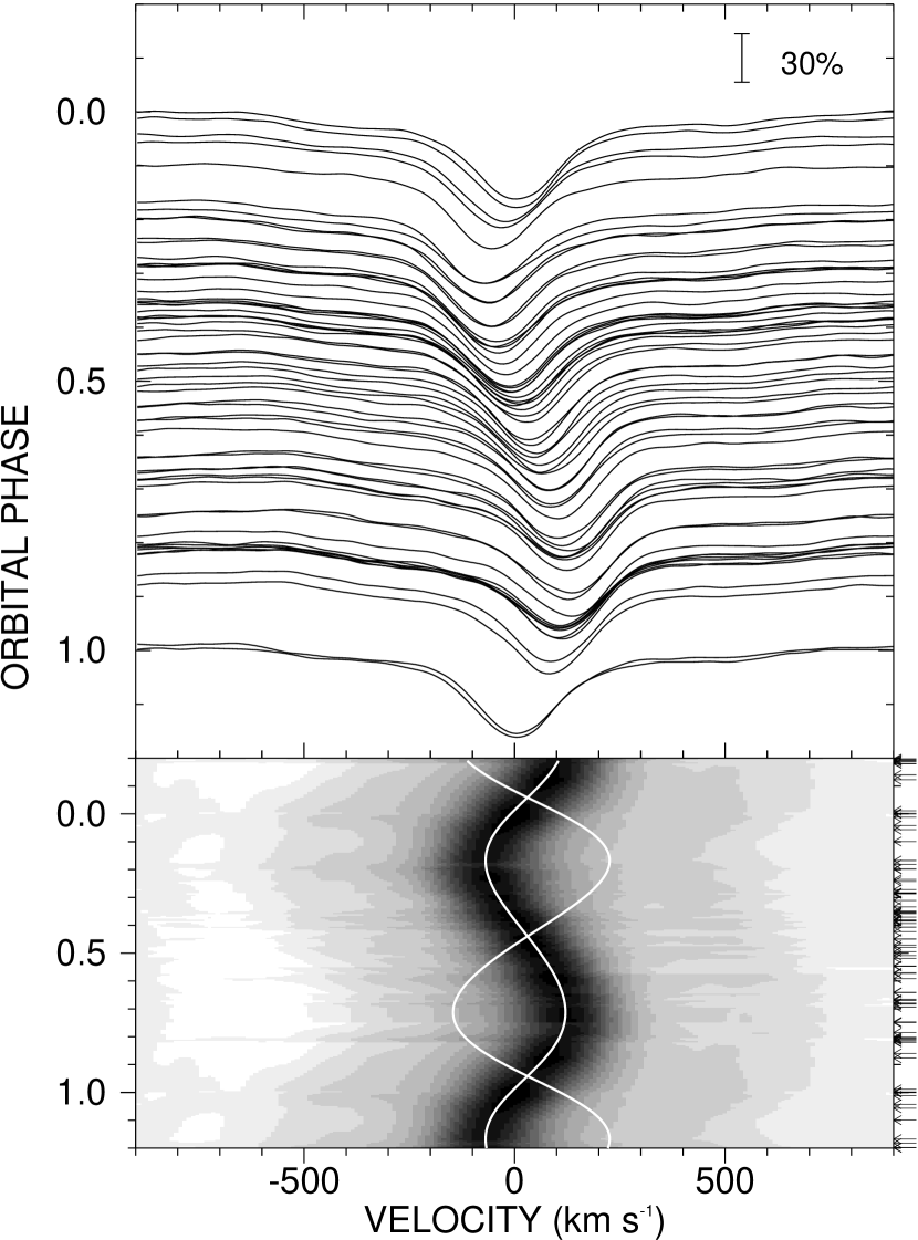
Figure 2:

Figure 3:

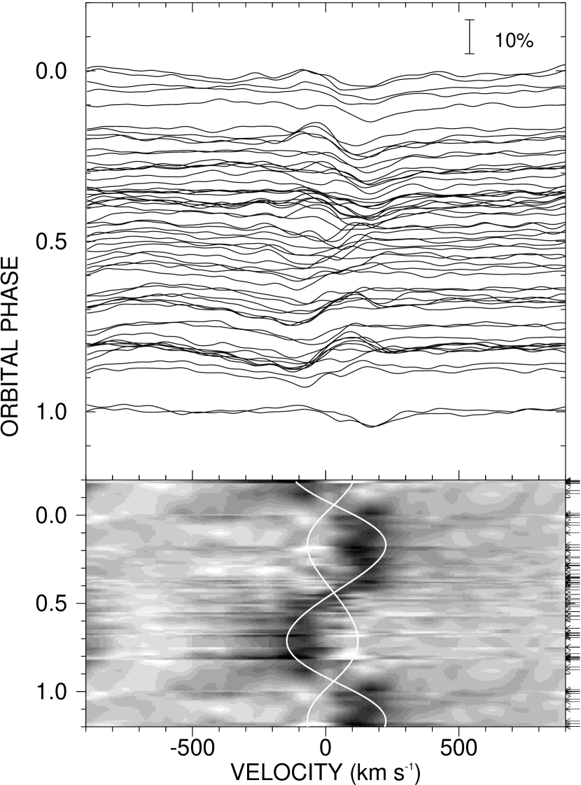
Figure 4:

Figure 5:

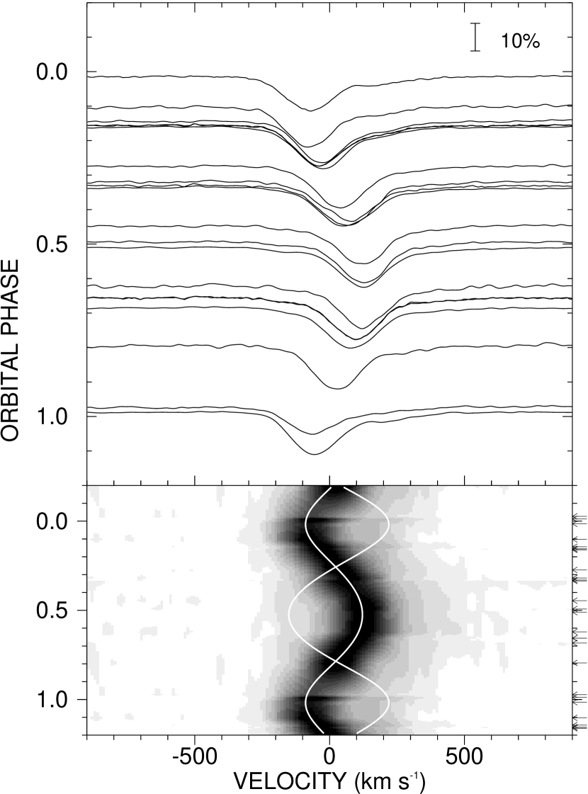
Figure 6:

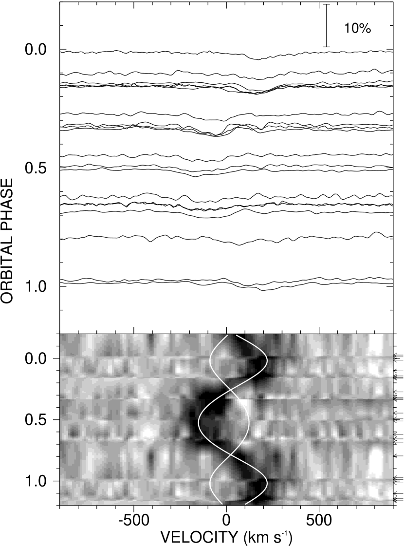
Figure 7:

Figure 8:

Figure 9:

Figure 10:

Figure 11:

Figure 12:

Figure 13:

Figure 14:

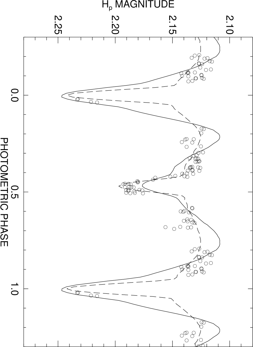
Figure 15:

References

- Bagnuolo et al. (1994) Bagnuolo, W. G., Jr., Gies, D. R., Hahula, M. E., Wiemker, R., & Wiggs, M. S. 1994, ApJ, 423, 446
- Bieging et al. (1989) Bieging, J. H., Abbott, D. C., & Churchwell, E. B. 1989, ApJ, 340, 518
- Blaauw (1991) Blaauw, A. 1991, in The Physics of Star Formation and Early Stellar Evolution, NATO Advanced Science Institutes (ASI) Series C, Vol. 342, ed. C. J. Lada & N. D. Kylafis (Dordrecht: Kluwer), 125
- Brown (1996) Brown, A. G. A. 1996, Ph.D. thesis, Univ. of Leiden
- Brown et al. (1994) Brown, A. G. A., de Geus, E. J., & de Zeeuw, P. T. 1994, A&A, 289, 101
- Curtiss (1914) Curtiss, R. H. 1914, Publ. Mich. Obs., 1, 118
- de Zeeuw et al. (1999) de Zeeuw, P. T., Hoogerwerf, R., de Bruijne, J. H. J., Brown, A. G. A., & Blaauw, A. 1999, AJ, 117, 354
- Fullerton (1990) Fullerton, A. W. 1990, Ph.D. thesis, Univ. of Toronto
- Galkina (1976) Galkina, T. S. 1976, Izvestiia Krymskaia Astrofiz. Obs., 54, 128
- Garhart et al. (1997) Garhart, M. P., Smith, M. A., Turnrose, B. E., Levay, K. L., & Thompson, R. W. 1997, International Ultraviolet Explorer New Spectral Image Processing System Information Manual, Version 2.0 (Greenbelt: NASA)
- Gies (1995) Gies, D. R. 1995, in IAU Symposium 163, Wolf-Rayet Stars: Binaries, Colliding Winds, Evolution, ed. K. A. van der Hucht & P. M. Williams (Dordrecht: Kluwer), 373
- Gies & Bolton (1986) Gies, D. R., & Bolton, C. T. 1986, ApJS, 61, 419
- Gies et al. (1999) Gies, D. R., et al. 1999, ApJ, 525, 420
- Harmanec (1988) Harmanec, P. 1988, Bull. Ast. Inst. Czech., 39, 329
- Harmanec (1998) Harmanec, P. 1998, A&A, 335, 173
- Harries et al. (1998) Harries, T. J., Hilditch, R. W., & Hill, G. 1998, MNRAS, 295, 386
- Hartkopf et al. (1993) Hartkopf, W. I., Mason, B. D., Barry, D. J., McAlister, H. A., Bagnuolo, W. G., Jr., & Prieto, C. M. 1993, AJ, 106, 352
- Hartmann (1904) Hartmann, J. 1904, ApJ, 19, 268
- Harvey et al. (1987) Harvey, A. S., Stickland, D. J., Howarth, I. D., & Zuiderwijk, E. J. 1987, Observatory, 107, 205
- Heger & Langer (2000) Heger, A., & Langer, N. 2000, ApJ, 544, 1016
- Heintz (1980) Heintz, W. D. 1980, ApJS, 44, 111
- Herrero et al. (1999) Herrero, A., Corral, L. J., Villamariz, M. R., & Martin, E. L. 1999, A&A, 348, 542
- Herrero et al. (2000) Herrero, A., Puls, J., & Villamariz, M. R., 2000, A&A, 354, 193
- Hnatek (1920) Hnatek, A. 1920, Astronomisches Nachrichten, 213, 17
- Howarth & Prinja (1989) Howarth, I. D., & Prinja, R. K. 1989, ApJS, 69, 527
- Howarth et al. (1997) Howarth, I. D., Siebert, K. W., Hussain, G. A. J., & Prinja, R. K. 1997, MNRAS, 284, 265
- Hutchings (1976) Hutchings, J. B. 1976, ApJ, 203, 438
- Jordan (1914) Jordan, F. C. 1914, Publ. Allegheny Obs., 3, 125
- Koch & Hrivnak (1981) Koch, R. H., & Hrivnak, B. J. 1981, ApJ, 248, 249
- Kurucz (1994) Kurucz, R. L. 1994, Solar Abundance Model Atmospheres for 0, 1, 2, 4, 8 km/s, Kurucz CD-ROM No. 19 (Cambridge, MA: Smithsonian Astrophysical Obs.)
- Liu et al. (1997) Liu, N., et al. 1997, ApJ, 485, 350
- Luyten et al. (1939) Luyten, W. J., Struve, O., & Morgan, W. W. 1939, Publ. Yerkes Obs., 7, 256
- Mason et al. (1998) Mason, B. D., Gies, D. R., Hartkopf, W. I., Bagnuolo, W. G., Jr., ten Brummelaar, T., & McAlister, H. A. 1998, AJ, 115, 821
- Massa (1989) Massa, D. 1989, A&A, 224, 131
- McAlister et al. (1983) McAlister, H. A., Hartkopf, W. I., Hendry, E. M., Campbell, B. G., & Fekel, F. C. 1983, ApJS, 51, 309
- McAlister et al. (1987) McAlister, H. A., Hartkopf, W. I., Hutter, D. J., & Franz, O. G. 1987, AJ, 93, 688
- McAlister et al. (1989) McAlister, H. A., Hartkopf, W. I., Sowell, J. R., Dombrowski, E. G., & Franz, O. G. 1989, AJ, 97, 510
- McAlister & Hendry (1982) McAlister, H. A., & Hendry, E. M. 1982, ApJS, 49, 267
- McAlister et al. (1993) McAlister, H. A., Mason, B. D., Hartkopf, W. I., & Shara, M. M. 1993, AJ, 106, 1639
- Meynet & Maeder (2000) Meynet, G., & Maeder, A. 2000, A&A, 361, 101
- Miczaika (1952) Miczaika, G. R. 1952, Zeitschrift fur Astrophysik, 30, 299
- Mochnacki & Doughty (1972) Mochnacki, S. W., & Doughty, N. A. 1972, MNRAS, 156, 51
- Monet (1980) Monet, D. G. 1980, ApJ, 237, 513
- Morbey & Brosterhus (1974) Morbey, C. L., & Brosterhus, E. B. 1974, PASP, 86, 455
- Natarajan & Rajamohan (1971) Natarajan, V., & Rajamohan, R. 1971, Kodaikanal Bull., 208
- Penny (1996) Penny, L. R. 1996, ApJ, 463, 737
- Penny et al. (1997) Penny, L. R., Gies, D. R., & Bagnuolo, W. G., Jr. 1997, ApJ, 483, 439
- Penny et al. (1999) Penny, L. R., Gies, D. R., & Bagnuolo, W. G., Jr. 1999, ApJ, 518, 450
- Penny et al. (2001) Penny, L. R., et al. 2001, ApJ, 548, 889
- Perryman (1997) Perryman, M. A. C. 1997, The Hipparcos and Tycho Catalogues (ESA SP-1200) (Noordwijk: ESA)
- Pismis et al. (1950) Pismis, P., Haro, G., & Struve, O. 1950, ApJ, 111, 509
- Prieur et al. (2001) Prieur, J.-L., Oblak, E., Lampens, P., Kurpinska-Winiarska, M., Aristidi, E., Koechlin, L., & Ruymaekers, G. 2001, A&A, 367, 865
- Reid et al. (1993) Reid, A. H. N., et al. 1993, ApJ, 417, 320
- Rountree & Sonneborn (1993) Rountree, J., & Sonneborn, G. 1993, Spectral Classification with the International Ultraviolet Explorer: An Atlas of B-type Spectra (NASA RP-1312) (Washington, DC: NASA)
- Runacres & Bloome (1996) Runacres, M. C., & Bloome, R. 1996, A&A, 309, 544
- Schaller et al. (1992) Schaller, G., Schaerer, D., Meynet, G., & Maeder, A. 1992, A&AS, 96, 269
- Schönberner & Harmanec (1995) Schönberner, D., & Harmanec, P. 1995, A&A, 294, 509
- Singh (1982) Singh, M. 1982, Ap&SS, 87, 269
- Tarasov et al. (1995) Tarasov, A. E., et al. 1995, A&AS, 110, 59
- Thaller (1997a) Thaller, M. L. 1997a, ApJ, 487, 380
- Thaller (1997b) Thaller, M. L. 1997b, Ph.D. dissertation, Georgia State Univ.
- Vanbeveren et al. (1998) Vanbeveren, D., van Rensbergen, W., & de Loore, C. 1998, The Brightest Binaries (Dordrecht: Kluwer)
- Voels et al. (1989) Voels, S. A., Bohannan, B., Abbott, D. C., & Hummer, D. G. 1989, ApJ, 340, 1073
- Wade & Rucinski (1985) Wade, R. A., & Rucinski, S. M. 1985, A&AS, 60, 471
- Walborn (1972) Walborn, N. R. 1972, AJ, 77, 312
- Walborn (1976) Walborn, N. R. 1976, ApJ, 205, 419
- Wellstein et al. (2001) Wellstein, S., Langer, N., & Braun, H. 2001, A&A, 369, 939
- Worley & Douglass (1997) Worley, C. E., & Douglass, G. G. 1997, A&AS, 125, 523