Interferometric Mapping of Magnetic Fields in Star-forming Regions II. NGC 2024 FIR 5

Abstract

We present the first interferometric polarization maps of the NGC 2024 FIR 5 molecular core obtained with the BIMA array at approximately 2^′′ resolution. We measure an average position angle of $-$60^∘$\pm$6^∘ in the main core of FIR 5 and 54^∘$\pm$9^∘ in the eastern wing of FIR 5. The morphology of the polarization angles in the main core of FIR 5 suggests that the field lines are parabolic with a symmetry axis approximately parallel to the major axis of the putative disk in FIR 5, which is consistent with the theoretical scenario that the gravitational collapse pulled the field lines into an hour-glass shape. The polarization percentage decreases toward regions with high intensity and close to the center of the core, suggesting that the dust alignment efficiency may decrease at high density. The plane-of-sky field strength can be estimated with the modified Chandrasekhar-Fermi formula, and the small dispersion of the polarization angles in FIR 5 suggests that the magnetic field is strong ($\gtrsim 2$ mG) and perhaps dominates the turbulent motions in the core.

1 Introduction

Magnetic fields are thought to play a significant role in all stages of star formation (e.g., recent reviews by Mouschovias & Ciolek 1999; Shu et al. 1999). However, the magnetic field is the most poorly measured quantity in the star formation process. Observations of the linear polarization from the thermal emission of magnetically aligned dust grains provide a relatively easy approach to explore the magnetic field morphology (Heiles et al. 1993). Such observations give the field direction in the plane of the sky perpendicular to the direction of polarization (Davis & Greenstein 1951; Roberge 1996).

Information on the magnetic field morphology is useful for testing the predictions of theoretical models and simulations. The standard star formation theory predicts certain morphological evolution of magnetic fields. Theory predicts that molecular clouds will tend to be flat with their minor axes parallel to the field lines, because magnetic fields prevent collapse perpendicular to the direction of the field lines (Mouschovias 1976). As contracting cores form, the field morphology achieves an “hourglass” shape with a collapsing accretion disk $\sim$100 AU at the “pinch” and a magnetically supported envelope $\sim$1000 AU (Fiedler & Mouschovias 1993; Galli & Shu 1993). Furthermore, the rotation of disks may twist field lines into the direction along the disk and form a toroidal morphology (Holland et al. 1996). Numerical simulations performed by Ostriker, Gammie, & Stone (1999) show that the field morphology is more random for larger ratios of the thermal to magnetic energy.

Because of the high sensitivity requirement in polarization observations, most previous observations of even the nearest star-forming regions have been made with single-dish telescopes whose large beams cover a region greater than the physical extent of protostellar cores. For example, the angular resolution of the James Clerk Maxwell Telescope (JCMT) at 850 $\mu$m is $\sim$14^′′, which corresponds to $\sim$6000 AU at the distance of the Orion Molecular Cloud. Therefore, in order to test theoretical models and simulations of star formation, it is essential to obtain high-resolution observations of magnetic fields. The best available approach to acquire high resolution information is to conduct interferometric observations. Pioneer interferometric polarization observations at millimeter wavelengths have been done with the Owens Valley Radio Observatory (Akeson & Carlstrom 1997). Recently, the Berkeley-Illinois-Maryland-Association millimeter array (BIMA) has been able to successfully provide extended polarization maps with high resolution up to 2^′′ (Rao et al. 1998; Girart, Crutcher, & Rao 1999; Lai et al. 2001, hereafter Paper I).

NGC 2024, a massive star formation region in the Orion B Giant Molecular Cloud (distance $\sim$ 415 pc: Anthony-Twarog 1982), is a good candidate to explore the magnetic field structure at small scales. It contains a luminous H ii region with a north-south molecular ridge at its center corresponding to the dust lane in the optical image. Mezger et al. (1988, 1992) identify seven dust cores in the molecular ridge at 1300 and 350 $\mu$m and assign designations using the acronym ’FIR’. They interpret these cores as isothermal protostars in the stage of free-fall contraction. However, detailed studies of FIR 4/5/6 show that these cores contain either a near-infrared source or strong outflows that are traditionally related to protostellar cores in a more evolved stage (Moore & Chandler 1989; Chandler & Carlstrom 1996). Our interest here focuses on the brightest core, FIR 5. With a highly collimated unipolar molecular outflow extended over $\sim$5^′ south of the core (Richer et al. 1992), FIR 5 appears to be the most evolved object among the FIR cores in NGC 2024. Continuum observations at 3 mm by Wiesemeyer et al. (1997) resolve FIR 5 into two compact cores, and they suggest FIR 5 is a binary disk with an envelope. The magnetic field structure in NGC 2024 has been mapped with VLA OH and H i Zeeman observations by Crutcher et al. (1999) and with far-infrared dust polarization by Dotson at al. (2000). Both observations have beam sizes larger than the FIR 5 core. Our observations provide new information on detailed field morphology in the FIR 5 core.

2 Observations and Data Reduction

The observations were carried out from 1999 March to 2001 February using nine BIMA antennas with 1-mm Superconductor-Insulator-Superconductor (SIS) receivers and quarter-wave plates. The digital correlator was set up to observe both continuum and the CO $J$=2$\rightarrow$1 line simultaneously. The continuum was observed with a 750 MHz window centered at 226.9 GHz in the lower sideband and a 700 MHz window centered at 230.9 GHz in the upper sideband. Strong CO $J$=2–1 line emission was isolated in an additional 50 MHz window in the upper sideband. The primary beam was $\sim$50^′′ at 1.3 mm wavelength. Data were obtained in the D, C, and B array configurations, and the projected baseline ranges were 4.5–20, 5–68, and 5–180 kilowavelengths. The integration time in the D, C, and B array was 3.4, 19.1, and 11 hours, respectively. The D-array observations were made first on 1999 March with a pointing center between NGC 2024 FIR 5 and FIR 6 ($\alpha_{2000}=5^{h}41^{m}45\fs 0$, $\delta_{2000}=-1\hbox{${}^{\circ}$}55\hbox{${}^{\prime}$}55\farcs 0$). Because the D-array data showed significant amount of polarized flux toward FIR 5 near the edge of the primary beam, the follow-up C- and B-array observations were therefore made with a pointing center at FIR 5 ($\alpha_{2000}=5^{h}41^{m}44\fs 35$, $\delta_{2000}=-1\hbox{${}^{\circ}$}55\hbox{${}^{\prime}$}42\farcs 0$).

The BIMA polarimeter and the calibration procedure are described in detail in Paper I (also see Rao et al. 2001, in preparation). The average instrumental polarization of each antenna was 5.6%$\pm$0.4% for our observations. The Stokes $I$ image of the continuum was made by mosaicing the B-, C-, and D-array data with Briggs’ robust weighting of 0.5 (Briggs 1995; Sault & Killeen 1998) to obtain a smaller synthesized beam (HPBW 2$\farcs$3$\times$1$\farcs$4, PA=9^∘) without losing significant amount of flux. D-array data were needed to recover the extended emission in order to obtain better measurements of the polarization percentage. The Stokes $Q$ and $U$ images were made with B- and C-array data only, because the precise pattern of the off-axis polarization across the primary beam is unknown. Rao et al. (1999) measured the off-axis instrumental polarization at selected positions and showed that it only provides an uncertainty less than 0.5% (comparable to the uncertainty of the leakages) within 4/5 of the primary beam; therefore, the off-axis polarization calibration was ignored. Natural weighting was used to produce the maps of the Stokes $Q$ and $U$ in order to obtain the highest S/N ratio, and the resulting synthesized beam was 2$\farcs$4$\times$1$\farcs$4 with PA=8^∘.

Maps of Stokes $Q$ and $U$ were deconvolved and binned to approximately half-beamwidth per pixel (1$\farcs$2$\times$0$\farcs$6) to reduce oversampling in our statistics. These maps were combined to obtain the linearly polarized intensity ($I_{p}$), the position angle ($\phi$), and the polarization percentage ($p$), along with their uncertainties as described in Section 2 of Paper I. When weighted with $I_{p}$, the average measurement uncertainty in the position angle for our observations was 6$\fdg$0$\pm$2$\fdg$3.

3 Results and Analysis

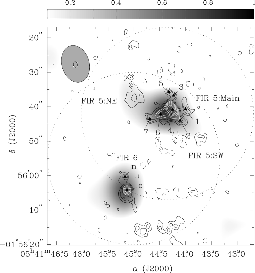
Figure 1: Stokes $I$ maps of NGC 2024 FIR 5 and FIR 6. The contours show the total intensity (Stokes $I$) in the B+C-array data at $-5,-3,3,5,8,12,17,23,30,40,50,60~{}\sigma$ levels (1$\sigma$ = 3.3  mJy beam^-1). The color of the contours is chosen to show better contrast on the background. The field of view is represented by the northern dotted circle. The grey-scale shows the D-array data and the field of view is the southern dotted circle. The grey ellipses in the upper left corner are the synthesized beams for these two sets of data, which are 1$\farcs$6$\times$1$\farcs$2 with PA=11^∘ for the B+C-array map and 11^′′$\times$8^′′ with PA=16^∘ for the D-array map. The triangles mark the positions of compact continuum sources identified in the B+C-array map (Table 1).

Figure 1 shows the B+C-array Stokes I map (contours) superposed on the D-array Stokes I map (grey-scale). The B+C-array map resolves FIR 5 and FIR 6 into several clumps with the highest resolution ever obtained (1$\farcs$6$\times$1$\farcs$2, PA=11^∘). The clumps with peak flux stronger than 7$\sigma_{I}$ ($1\sigma_{I}$ = 3.3  mJy beam^-1) are named and tabulated in Table 1. Figure 2 displays the mosaiced map of NGC 2024 FIR 5 overlaid with polarization vectors. This map contains B, C, and D array data. Polarization vectors are plotted at positions where the observed linearly polarized intensity is greater than 3$\sigma_{I_{p}}$ (1$\sigma_{I_{p}}$ = 2.1  mJy beam^-1) and the total intensity is greater than 3$\sigma_{I}$ (1$\sigma_{I}$ = 7.4  mJy beam^-1; note that $\sigma_{I}$ is dominated by incomplete deconvolution rather than thermal noise). Under these criteria, the polarized emission extends over an area of $\sim$8 beam sizes. Table 2 lists the polarization measurements in NGC 2024 FIR 5 at selected positions separated by approximately the synthesized beamsize. The distributions and the model fitting of the polarization angle are plotted in Figure 3 and Figure 4 respectively, and the distribution of the polarization percentage is shown in Figure 5.

3.1 Continuum and Polarized Emission

The continuum emission of FIR 5 can be separated into three main components – FIR 5:Main, FIR 5:NE, and FIR 5:SW (Figure 1). FIR 5:Main are resolved into seven clumps, and the seven clumps are assigned designations with ’LCGR’ (Table 1). Only the two brightest clumps (FIR 5:LCGR 4 and 6) were previously identified at 96 GHz (Wiesemeyer et al. 1997; note that we have renamed these two clumps). Wiesemeyer et al. (1997) suggested that FIR 5 is a binary disk; however, our high resolution data present complex morphology in FIR 5. Our data also show that the continuum of FIR 6 consists of two compact sources. The three main components of FIR 5 and the two compact sources of FIR 6 are clearly seen in the 450 $\mu$m continuum maps of Visser et al. (1998), suggesting that they are dust dominated sources.

Figure 2 shows that our detection of the polarized flux in FIR 5 is mainly distributed in a $\sim$10^′′$\times$4^′′ strip along the major axis of FIR 5:LCGR 4 extending into FIR 5:LCGR 2, which is roughly perpendicular to the disk previously proposed by Wiesemeyer et al. (1997). The peak of the polarized flux occurs at a position about 1$\farcs$8 north of the continuum peak between FIR 5:LCGR 3 and 4. Detections with $I_{p}>3\sigma_{I_{p}}$ were also made toward positions near FIR 5:LCGR 7 and in FIR 5:NE.

3.2 Polarization Angle Distribution

The histogram of polarization angles in FIR 5 is shown in Figure 3. Most of the polarization detected is associated with FIR 5:LCGR 4. Toward this source the average position angle is $-$60^∘$\pm$6^∘, and the angles appear to decrease from south to north from $-$7^∘ to $-$71^∘. Compact polarization is also observed associated with FIR 5:NE and FIR 5:LCGR 7. Both these sources show a similar position angle (average = 54^∘$\pm$9^∘) which is very distinct from that of the vectors in FIR 5:LCGR 4. Our results are consistent with recent JCMT observations at 850 $\mu$m, which also show $\phi\sim$ 50^∘ in FIR 5:NE, low polarization around FIR 5:LCGR 6, and $\phi\sim$ $-$60^∘ in FIR 5:LCGR 4 (Matthews et al. 2001, private communication).

Since the magnetic field direction inferred from the dust polarization is perpendicular to the polarization vectors, the variation of the polarization angles around FIR 5:LCGR 4 suggests that the magnetic field lines are curved. The curved field lines can be successfully modeled with a set of parabolas with the same focal point, and the best model with minimum $\chi^{2}$ is presented in Figure 4. The symmetry axis of the best model is at $-$77^∘, which is consistent with the position angle of the line connecting FIR 5: d and f at $-$67^∘. The histogram in Figure 4 shows the distribution of the deviation between our measurements and the best model, which shows a Gaussian-like distribution with a dispersion of $\delta\phi_{obs}$=9$\fdg$2$\pm$3$\fdg$3. After deconvolving the measurement uncertainty in this region ($\sigma_{\phi}=5\fdg 8\pm 2\fdg 2$) from the observed dispersion, we obtain the intrinsic dispersion of the polarization angles $\delta\phi=7\fdg 1\pm 2\fdg 5$.

3.3 Polarization Percentage Distribution

The average polarization percentage is 6.0%$\pm$1.5% in the main core and 10.5%$\pm$4.7% toward the eastern side of FIR 5. The polarization percentage distribution is plotted in Figure 5. These plots show that the polarization percentage decreases toward regions of high intensity as well as toward the cloud center. Based on the apparent close correlation in both Figure 5(a) and 5(b), we perform a least-squares fit on $\log_{10}p$ versus $\log_{10}I$ and $p$ versus the distance from the peak of FIR 5:LCGR 4 ($R$). We obtain the following results: (1) for all data points, $\log_{10}p=(-1.88\pm 0.01)-(0.83\pm 0.01)\times\log_{10}I$ with a correlation coefficient of $-$0.86, and (2) in the main core, $p=(3.60\pm 0.63)\%+(1.45\pm 0.16)R$ with a correlation coefficient of 0.97. Because higher intensity and smaller radius both imply higher density, our results suggest that the polarization percentage decreases toward the high density region. This conclusion is consistent with what we reported in Paper I for the W51 e1/e2 cores, and our interpretation was the decrease of the dust alignment efficiency toward high density regions.

4 Discussion

4.1 Magnetic Field and Molecular Core Morphology

In §3.2, we showed that the field lines in NGC 2024 FIR 5 can be modeled with a set of parabolas which may represent part of an hour-glass shape. The reason that the rest of the hour-glass shape is not detected could be due to the relatively lower dust column density to the east of the region where polarization has been detected. The hour-glass geometry has been predicted by theoretical work and simulations (Fiedler & Mouschovias 1993; Galli & Shu 1993). When enough matter collapses along field lines and forms a disk-like structure, the gravity in the direction along the major axis of the disk would eventually overcome the supporting forces and pull the field lines into an hour-glass shape. Observations of magnetic fields have found several cases consistent with this geometry, such as in W3 (Roberts et al. 1993; Greaves, Murray, & Holland 1994), OMC-1 (Schleuning 1998), and NGC 1333 IRAS 4A (Girart, Crutcher, & Rao 1999). Our results in NGC  2024 FIR 5 provide a possible supporting example to the theoretical models at a small scale of few thousand AU. This scale is much smaller than the hour-glass shapes observed in W3 and OMC-1 ($10^{4}-10^{5}$ AU), and is comparable to that in NGC 1333 IRAS 4A.

The symmetry axis of our hour-glass model is approximately parallel to the binary disk previously proposed by Wiesemeyer et al. (1997). Such a coincidence could be an indirect evidence for the existence of a collapsing disk. Although our high resolution map shows that FIR 5:Main is more complicated than a binary disk, it is still possible that there is an east-west disk consisting of four clumps (FIR 5:LCGR 1, 4, 6, and 7), with the remaining three clumps either collapsing into the disk or being ejected through outflows. FIR 5:LCGR 2 is at $\sim-$145^∘ direction with respect to FIR 5:LCGR 4, which is close to the unipolar outflow at $\sim-$170^∘. Since outflows could be deflected by magnetic fields away from the protostellar cores (Girart, Crutcher, & Rao 1999), it is possible that FIR 5:LCGR 2 traces the direction of the outflow near the central core. Further high resolution kinematic study is needed to examine the above speculation.

4.2 Estimation of the Magnetic Field Strength

Although the magnetic field strength cannot be directly inferred from polarization of dust emission, Ostriker, Stone, & Gammie (2001) show that the Chandrasekhar-Fermi formula (Chandrasekhar & Fermi 1953) modified with a factor of 0.5 can provide accurate estimates of the plane-of-sky field strength under strong field cases ($\delta\phi\leq 25\hbox{${}^{\circ}$}$) for their simulations of magnetic turbulent clouds. Therefore, the projected field strength ($B_{p}$) can be expressed as

$$B_{p}=0.5\sqrt{4\pi\bar{\rho}}~{}~{}\frac{\delta v_{los}}{\delta\phi}=8.5~{}\frac{\sqrt{n_{H_{2}}/(10^{6}{\,\rm cm}^{-3})}~{}\Delta v/{\,\rm km~{}s}^{-1}}{\delta\phi/1\hbox{${}^{\circ}$}}~{}~{}{\rm mG},$$ (1)

where $\bar{\rho}$ is the average density, $\delta v_{los}$ is the rms line-of-sight velocity, the number density of molecular hydrogen $n_{H_{2}}=2.33~{}m_{H}n_{H}$, and the linewidth $\Delta v=\sqrt{8\ln 2}~{}\delta v_{los}$.

To estimate $B_{p}$ in NGC 2024 FIR 5, we must first carefully determine the density of the dust core and the turbulent linewidth. Mezger et al. (1992) derived high density ($n_{H}\sim 10^{8}$ cm^-3) in FIR 1-7 from dust emission, but their value is significantly higher than that derived from molecular studies ($\sim$10⁶ cm^-3 from CS: Schulz et al. 1991; $\sim$10⁷ cm^-3 from C¹⁸O: Wilson, Mehringer, & Dickel 1995). It is possible that depletion of molecules in the dense core causes molecules to only trace the envelope of the dense core; on the other hand, Chandler & Carlstrom (1996) showed that the kinetic temperature in the FIR cores is higher than what Mezger et al. (1992) assume, implying a lower density. Mangum, Wootten, & Barsony (1999) studied the kinetic temperature in NGC 2024 with multi-line observations of formaldehyde (H₂CO), and their results supported the arguments of Chandler & Carlstrom (1996). We therefore adopt $n_{H_{2}}\sim 2\times 10^{6}$ cm^-3 for FIR 5 from Mangum, Wootten, & Barsony’s large velocity gradient (LVG) calculation. We also adopt a weighted linewidth of $\Delta v=2.04\pm 0.03$ km s^-1 at the position at the peak of FIR 5 from Mangum, Wootten, & Barsony (1999). Note that, just as for other molecules, the peak of H₂CO emission does not coincide with the continuum peak; therefore, the H₂CO emission may come from the envelope of the FIR 5. This may be an advantage because the H₂CO linewidth is less likely contaminated by the possible dynamical motions in the core and better represents the turbulent motion.

In §3.2, we calculated the angle dispersion $\delta\phi=7\fdg 1\pm 2\fdg 5$ after taking out the systematic field structure in order to identify the dispersion purely from the Alfvénic motion. Along with the parameters discussed in the previous paragraph, we obtain $B_{p}\sim$3.5 mG. We can also calculate the lower limit of $B_{p}$ using the largest angle dispersion, which is the dispersion before taking out the parabolic model ($\delta\phi=$13$\fdg$1$\pm$4$\fdg$6); thus, $B_{p,min}\sim$1.9 mG. Our estimate of the plane-of-sky field strength is much larger than the line-of-sight field strength measured by Crutcher et al. (1999) from OH Zeeman observation, which is $\sim 65\mu$G at FIR 5. Except in the unlikely case that the magnetic field direction lies almost on the plane of the sky, the low field strength detected with the Zeeman measurement can be explained by (1) the beam-averaging over small scale field structure, and/or (2) that OH line does not trace high density region of the dust cores.

4.3 Turbulent Energy vs. Magnetic Energy

The small dispersion of the polarization angles observed by us may imply that the turbulent motion is not strong enough to disturb the magnetic field structure. In order to quantitatively discuss the the relative importance of the turbulent and magnetic energy in NGC 2024 FIR 5, we calculate the ratio of the turbulent to magnetic energy

$$\beta_{turb}\equiv\frac{\sigma_{turb}^{2}}{V_{A}^{2}},$$ (2)

where $\sigma_{turb}$ is the turbulent linewidth and $V_{A}=|\bf{B}|/\sqrt{4\pi\bar{\rho}}$ is the Alfvén speed. Statistically, $<B_{p}^{2}>=\frac{2}{3}~{}|\bf{B}|^{2}$, thus $V_{A}$ can be estimated from Eq. (1). Therefore,

$$\beta_{turb}\approx\frac{8}{3}~{}\frac{\sigma_{turb}^{2}}{\delta v_{los}^{2}}~{}\delta\phi^{2}.$$ (3)

In the general conditions prevalent in molecular clouds, the thermal linewidth $\sigma_{thermal}$ is much smaller than the turbulent linewidth, so $\delta v_{los}^{2}=\sigma_{turb}^{2}+\sigma_{thermal}^{2}\approx\sigma_{turb}^{2}$. The ratio of the turbulent to magnetic energy simply depends on the polarization angle dispersion,

$$\beta_{turb}\approx\frac{8}{3}~{}\delta\phi^{2}=8\times 10^{-4}(\frac{\delta\phi}{1\hbox{${}^{\circ}$}})^{2}.$$ (4)

The 0.5 factor in Eq (1) was obtained under the assumption that the dust alignment efficiency is uniform throughout the cloud. If dust alignment efficiency is lower in the regions with higher density as we suggest in §3.3, $\beta_{turb}$ would be larger for the same $\delta\phi$ and the correction depends on the degree of depolarization. For our case, the most conservative estimate of the angle dispersion is $\delta\phi<13\fdg 1$, which leads to a small turbulent to magnetic energy ratio, $\beta_{turb}<0.14$. Therefore, the magnetic field most likely dominates the turbulent motion in the core region of NGC 2024 FIR 5. This is also the case in W51 e1/e2 (see Paper I).

5 Conclusions

High-resolution polarization observations are needed to explore the detailed magnetic field structure in star-forming cores. We have obtained a continuum map of NGC 2024 FIR 5 and FIR 6 and a polarization map of NGC 2024 FIR 5 with the highest resolution ever obtained ($\sim$2^′′). Our observations resolve FIR 5 and FIR 6 into several continuum clumps. The information revealed by our polarization observations of FIR 5 are summarized below:

• Extended polarization is detected associated with the main core at $-$60^∘$\pm$6^∘. Compact polarization is also observed toward the eastern side of FIR 5 at 54^∘$\pm$9^∘. The polarization is low between these two regions and the secondary intensity peak of FIR 5 has an upper limit of 6%.

• The magnetic field lines in the core are systematically curved with a symmetry axis close to the major axis of a putative disk. This is consistent with an hour-glass morphology for the magnetic fields predicted by theoretical works.

• The polarization percentage decreases toward regions with high intensity and short distance to the center of the core. The tight correlations imply that the depolarization is a global effect and may be caused by the decrease of the dust alignment efficiency in high density regions.

• The small dispersion of the polarization angles in the core suggests that the magnetic field is strong ($\gtrsim$ 2 mG) and the ratio of the turbulent to magnetic energy is small ($\beta_{turb}<0.14$). Therefore, the magnetic field most likely dominates turbulent motions in NGC 2024 FIR 5.

Table 1: Compact continuum sources in FIR 5 and FIR 6

	$\alpha_{2000}$	$\delta_{2000}$	$I$	$p$
Source	${}^{h}~{}~{}^{m}~{}~{}~{}^{s}~{}~{}$	∘   ′   ′′	( mJy beam-1)	(%)
FIR 5:LCGR 1	5 41 44.00	-1 55 40.7	46	$<$ 17
FIR 5:LCGR 2	5 41 44.10	-1 55 44.0	64	10.3
FIR 5:LCGR 3	5 41 44.23	-1 55 36.8	39	$<$ 25
FIR 5:LCGR 4	5 41 44.25	-1 55 40.8	293	3.8
FIR 5:LCGR 5	5 41 44.32	-1 55 35.7	40	$<$ 21
FIR 5:LCGR 6	5 41 44.48	-1 55 42.2	107	$<$ 6
FIR 5:LCGR 7	5 41 44.69	-1 55 43.5	55	$<$ 14
FIR 6 c	5 41 45.13	-1 56 04.2	67	–
FIR 6 n	5 41 45.17	-1 56 00.3	26	–

Table 2: Polarization Measurements in NGC 2024 FIR 5

Position	Stokes $I$	Polarization	Polarization	Note
(′′,′′)	( mJy beam-1)	Percentage(%)	Angle (∘)
(-0.3, 4.5)	26.6$\pm$7.3	23.1$\pm$9.5	-72$\pm$9
(-1.1, 3.0)	132.8$\pm$7.3	18.7$\pm$1.9	-71$\pm$2	Polarization Peak
(-1.2, 1.2)	300.6$\pm$7.3	3.9$\pm$0.7	-64$\pm$5	Intensity Peak
(-1.8, 4.5)	41.9$\pm$7.3	19.5$\pm$6.1	-66$\pm$7
(-2.6, 1.2)	153.7$\pm$7.3	4.9$\pm$1.4	-39$\pm$8
(-2.6,-0.8)	137.1$\pm$7.3	6.5$\pm$1.6	-39$\pm$7
(-2.6,-2.7)	45.6$\pm$7.3	15.4$\pm$5.2	- 8$\pm$9
(-3.9,-0.9)	53.2$\pm$7.3	20.0$\pm$4.8	-42$\pm$6
(-4.8,-2.4)	39.1$\pm$7.3	17.3$\pm$6.3	-39$\pm$9
(10.2, 8.9)	31.7$\pm$7.3	27.1$\pm$9.2	63$\pm$7	FIR 5:NE
( 4.1,-0.5)	75.7$\pm$7.3	9.3$\pm$2.9	31$\pm$9	near FIR 5:LCGR 7
–	–	6.0$\pm$1.5	-60$\pm$6	average of the main core
–	–	10.5$\pm$4.7	54$\pm$9	average of the eastern side of FIR 5

Figure 2: Polarization map of NGC 2024 FIR 5. The contours represent the mosaiced Stokes $I$ map at $-5,-3,3,5,10,20,30,40\sigma$ levels. The 1 $\sigma$ noise level of Stokes $I$ is 7.3  mJy beam^-1 and the beam HPBW is 2$\farcs$3$\times$1$\farcs$4 with PA=9^∘. The line segments are polarization vectors (E-vectors), and their lengths are proportional to the polarization percentage with a scale of 10% per arcsec length. The triangles mark the positions of compact continuum sources listed in Table 1.

Figure 3: The distribution of the position angles of the polarization vectors in NGC 2024 FIR 5. The vertical axis is the total number of the measurements in the bin.

Figure 4: Model fitting of the magnetic field morphology using a set of parabolas with the same focus point. The line segments are polarization vectors which are perpendicular to the magnetic field directions. The dotted lines shows the least-squares model, the dashed line is the symmetry axis, and the star is the common focus point. The histogram shows the distribution of the deviation between the field directions and the model.

Figure 5: Polarization percentage distribution. The filled dots represent the data associated with the main core of FIR 5, and the open dots represent the data associated with the eastern side of FIR 5. The dotted lines are the best least-squares fits for the set of data. (a) shows the polarization percentage vs. the total intensity. The error bar of each data point is the measurement uncertainty. We plot the total intensity increasing to the left to emphasize that high intensity corresponds to short distance to the center of the core. (b) shows the polarization percentage vs. the distance from the FIR 5:LCGR 4 peak. Data with R greater than 6^′′ are not shown, because the average polarized intensity is lower than 1.5$\sigma_{I_{p}}$. The error bar in radius shows the range over which the data are averaged and the error bar in $p$ is the standard deviation of the data in the range.

References

- (1) Akeson, R. L., & Carlstrom, J. E. 1997, ApJ, 491, 254
- Anthony-Twarog (1982) Anthony-Twarog, B. J. 1982, AJ, 87, 1213
- (3) Briggs, D. S. 1995, PhD Dissertation, The New Mexico Institute of Mining and Technology (available at the website http://www.aoc.nrao.edu/ftp/dissertations/dbriggs/diss.html)
- Chandler & Carlstrom (1996) Chandler, C. J., & Carlstrom, J. E. 1996, ApJ, 466, 338
- (5) Chandrasekhar, S., & Fermi, E. 1953, ApJ, 118, 113
- Crutcher, Roberts, Troland, & Goss (1999) Crutcher, R. M., Roberts, D. A., Troland, T. H., & Goss, W. M. 1999, ApJ, 515, 275
- (7) Davis, L., & Greenstein, J. L. 1951, ApJ, 114, 209
- (8) Dotson, J. L., Davidson, J., Dowell, C. D., Schleuning, D. A., & Hildebrand, R. H. 2000, ApJS, 128, 335
- (9) Fiedler, R. A., & Mouschovias, T. Ch. 1993, ApJ, 415, 680
- (10) Galli, D., & Shu, F. H. 1993, ApJ, 417, 243
- (11) Girart, J. M., Rao, R., & Crutcher, R. M. 1999, ApJ, 525, 109
- Greaves, Murray, & Holland (1994) Greaves, J. S., Murray, A. G., & Holland, W. S. 1994, A&A, 284, L19
- (13) Heiles, C., Goodman, A. A., McKee, C. F., & Zweibel, E. G. 1993, in Protostars and Planets III, eds. M. Matthews, & E. Levy (Tuscon: University of Arizona Press), 279
- (14) Holland, W. S., Greaves, J. S., Ward-Thompson, D., & Andre, P. 1996, A&A, 309, 267
- (15) Lai, S.-P., Crutcher, R. M., Girart, J. M., & Rao, R. 2001, to be published in the ApJ November 10, 2001 issue (Paper I)
- (16) Lazarian, A., Goodman, A. A., & Myers, P. C. 1997, ApJ, 490, 273
- (17) Leahy, P., VLA Scientific Memoranda No. 161
- Mangum, Wootten, & Barsony (1999) Mangum, J. G., Wootten, A., & Barsony, M. 1999, ApJ, 526, 845
- Mauersberger et al. (1992) Mauersberger, R., Wilson, T. L., Mezger, P. G., Gaume, R., & Johnston, K. J. 1992, A&A, 256, 640
- Mezger et al. (1988) Mezger, P. G., Chini, R., Kreysa, E., Wink, J. E., & Salter, C. J. 1988, A&A, 191, 44
- Mezger et al. (1992) Mezger, P. G., Sievers, A. W., Haslam, C. G. T., Kreysa, E., Lemke, R., Mauersberger, R., & Wilson, T. L. 1992, A&A, 256, 631
- Moore & Chandler (1989) Moore, T. J. T., & Chandler, C. J. 1989, MNRAS, 241, 19P
- (23) Mouschovias, T. Ch. 1976, ApJ, 207, 141
- (24) Mouschovias, T. Ch., & Ciolek, G. E. 1999, in The Origin of Stars and Planetary Systems, eds. C. J. Lada & N. D. Kylafis (Kluwer Academic Press), 305
- Ostriker, Gammie, & Stone (1999) Ostriker, E. C., Gammie, C. F., & Stone, J. M. 1999, ApJ, 513, 259
- (26) Ostriker, E. C., Stone, J. M., & Gammie, C. F. 2001, ApJ, 546, 980
- (27) Rao, R., Crutcher, R. M., Plambeck, R. L., & Wright, M. C. H. 1998, ApJ, 502, L75
- (28) Rao, R. 1999, Ph.D. Dissertation, University of Illinois at Urbana-Champaign
- (29) Rao, R., Crutcher, R. M., Girart, J. M., Lai, S.-P., Wright, M. C. H., & Plambeck, R. L. 2001, in preparation
- Richer, Hills, & Padman (1992) Richer, J. S., Hills, R. E., & Padman, R. 1992, MNRAS, 254, 525
- (31) Roberge, W. G. 1996, ASP Conf. Ser. 97: Polarimetry of the Interstellar Medium, 401
- Roberts, Crutcher, Troland, & Goss (1993) Roberts, D. A., Crutcher, R. M., Troland, T. H., & Goss, W. M. 1993, ApJ, 412, 675
- (33) Sault, R. J., & Killeen, N. E. B. 1998, Miriad Users Guide (available at the website http://www.atnf.csiro.au/computing/software/miriad)
- (34) Sault, R. J., Teuben, P. J., & Wright, M. C. H. 1995, ASP Conf. Ser. 77: Astronomical Data Analysis Software and Systems IV, 4, 433
- Schleuning, (1998) Schleuning, D. A. 1998, ApJ, 493, 811
- Schulz, Guesten, Zylka, & Serabyn (1991) Schulz, A., Guesten, R., Zylka, R., & Serabyn, E. 1991, A&A, 246, 570
- (37) Shu, F. H., Allen, A., Shang, H., Ostriker, E. C., & Li, Z. 1999, in The Origin of Stars and Planetary Systems, eds. C. J. Lada & N. D. Kylafis (Kluwer Academic Press),193
- (38) Thompson, A. R., Moran, J. M., & Swenson, G. W. 1986, Interferometry and Synthesis in Radio Astronomy (New York: Wiley)
- Visser, Richer, Chandler, & Padman (1998) Visser, A. E., Richer, J. S., Chandler, C. J., & Padman, R. 1998, MNRAS, 301, 585
- Wiesemeyer, Guesten, Wink, & Yorke (1997) Wiesemeyer, H., Guesten, R., Wink, J. E., & Yorke, H. W. 1997, A&A, 320, 287
- Wilson, Mehringer, & Dickel (1995) Wilson, T. L., Mehringer, D. M., & Dickel, H. R. 1995, A&A, 303, 840