A new source detection algorithm using FDR

A. M. Hopkins¹¹affiliation: Hubble Fellow ²²affiliation: email: ahopkins@phyast.pitt.edu (1), C. J. Miller(2), A. J. Connolly(1), C. Genovese(3), R. C. Nichol(2), L. Wasserman(3) 1. Dept. of Physics and Astronomy, University of Pittsburgh, 3941 O’Hara Street, Pittsburgh, PA 15260 2. Dept. of Physics, Carnegie Mellon University, 5000 Forbes Avenue, Pittsburgh, PA 15213 3. Dept. of Statistics, Carnegie Mellon University, 5000 Forbes Avenue, Pittsburgh, PA 15213

Abstract

The False Discovery Rate (FDR) method has recently been described by Miller et al. (2001), along with several examples of astrophysical applications. FDR is a new statistical procedure due to Benjamini & Hochberg (1995) for controlling the fraction of false positives when performing multiple hypothesis testing. The importance of this method to source detection algorithms is immediately clear. To explore the possibilities offered we have developed a new task for performing source detection in radio-telescope images, Sfind 2.0, which implements FDR. We compare Sfind 2.0 with two other source detection and measurement tasks, Imsad and SExtractor, and comment on several issues arising from the nature of the correlation between nearby pixels and the necessary assumption of the null hypothesis. The strong suggestion is made that implementing FDR as a threshold defining method in other existing source-detection tasks is easy and worthwhile. We show that the constraint on the fraction of false detections as specified by FDR holds true even for highly correlated and realistic images. For the detection of true sources, which are complex combinations of source-pixels, this constraint appears to be somewhat less strict. It is still reliable enough, however, for a priori estimates of the fraction of false source detections to be robust and realistic.

methods: data analysis — methods: statistical — techniques: image processing

1 Introduction

Detecting and measuring the properties of objects in astronomical images in an automated fashion is a fundamental step underlying a growing proportion of astrophysical research. There are many existing tasks, some quite sophisticated, for performing such analyses. Regardless of the wavelength at which an image has been made however, each of these tasks has one thing in common: A threshold needs to be defined above which pixels will be believed to belong to real sources.

Defining an appropriate threshold is a complex issue and, owing to the unavoidable presence of noise, any chosen threshold will result in some true sources being overlooked and some false sources measured as real. Varying the chosen threshold to one extreme or the other will minimise one of these types of error at the expense of maximising the other. Clearly choosing a threshold to jointly minimise both types of error is not trivial, but even more problematic is that it is not even clear that one can, a priori, make a well defined estimate of the magnitude of each type of error. Typically this is done by comparing measured source counts with existing estimates for the expected number of sources. This is an unsatisfactory solution for surveys reaching to new sensitivity limits, or at previously uninvestigated wavelengths (where there can be no estimate of the expected number of sources from existing studies), and also for small area imaging where the properties of large populations are affected by clustering or small number statistics.

Throughout this paper we shall use the terms ‘source-pixel’ to mean a pixel in an image which is above some threshold, and thus assumed to be part of a true source. The term ‘source’ shall be used to mean a contiguous collection of ‘source-pixels’ which corresponds to an actual astronomical object, a star or galaxy for example, whose properties we are interested in measuring. In this work we concentrate on radio images, specifically images produced by radio interferometers. We emphasise, though, that all of the conclusions presented here are valid for any pixelized map where the ‘null hypothesis’ is known at each pixel. Throughout this paper the null hypothesis is taken to be the ‘sky background’ at each pixel (after the image is normalized).

Now consider the following possible criteria applied to some chosen threshold: (1) That there be no falsely discovered source-pixels; (2) That the proportion of falsely discovered source-pixels be some small fraction of the total number of pixels (background plus source); (3) That the fraction of false positives (i.e. the number of falsely discovered sources over the total number of discovered sources) be small. The first of these can be achieved by using a very high threshold called the Bonferroni threshold (Miller et al., 2001). This threshold is rarely used since, although guaranteeing no false detections, it detects so few real sources. The second criterion is most often applied in astronomy, and can be achieved by simply choosing the appropriate significance threshold. A threshold of $3\sigma$ , for example, ensures that $0.1\%$ of the total number of pixels are falsely discovered. Unfortunately this is not the same as a constraint on the fraction of false detections compared to total number of detections. This quantity is a more meaningful measure to use in defining a threshold for the following reason. Consider a $3\sigma$ threshold in an image composed of $10^{6}$ pixels ( $1000\times 1000$ ) and containing only Gaussian noise. This would yield, on average, 1000 pixels above the threshold. If real sources are also present, these 1000 pixels appear as false source-pixels, and if it happens that only 2000 pixels are measured as source-pixels, then half the detections are spurious! If many more true source-pixels are present, of course, this threshold may be quite adequate.

The third criterion defines a more ideal threshold. Such a threshold allows one to specify a priori the maximum number of false discoveries, on average, as a fraction of the total number of discoveries. Such a method should be independent of the source distribution (i.e., it will adapt the threshold depending on the number and brightness of the sources). The False Discovery Rate (FDR) method (Benjamini & Hochberg, 1995; Benjamini & Yekutieli, 2001; Miller et al., 2001) does precisely this, selecting a threshold which controls the fraction of false detections. We have implemented the FDR technique in a task for detecting and measuring sources in images made with radio telescopes.

Radio images were chosen for the current analysis for several reasons, including previous experience at coding of radio source detection tasks, but also since the conservative nature of constructing many radio source catalogues allows the value of this method to be emphasised. Traditionally radio source catalogues are constructed in a fashion aimed at minimising spurious sources, accomplished by selecting a very conservative threshold, which is usually $5\sigma$ or even $7\sigma$ . This is partly driven by the difficulty of completely removing residual image artifacts such as sidelobes of bright sources, even after applying very sophisticated image reconstruction methods, and the desire to avoid classifying these as sources. Many of the issues surrounding radio source detection are described by White et al. (1997). While such a conservative approach may minimise false detections, it has the drawback of not detecting large numbers of real, fainter, sources important in many studies of the sub-mJy and $\mu$ Jy populations, for example. An FDR defined threshold may allow many more sources to be included in a catalogue while providing a quantitative constraint to be placed on the fraction of false detections.

Table 1 briefly describes the algorithms used in some common radio source detection and measurement tasks. There is much similarity in the selection of tasks available within the two primary image analysis packages, aips (Astronomical Image Processing System¹¹1aips is a product of the National Radio Astronomy Observatory) and miriad (Multichannel Image Reconstruction, Image Analysis and Display²²2miriad is a product of the Berkeley Illinois Maryland Association), as alluded to in the summaries given in this table, although the specifics of each such task certainly differ to a greater or lesser extent. In addition to these packages, aips++ also has a image measurement task, imagefitter, similar in concept to the Imfit tasks in aips and miriad. A stand-alone task, SExtractor (Bertin & Arnouts, 1996), is used extensively in image analysis for detecting and measuring objects, primarily in images made at optical wavelengths. Given the flexibility of the SExtractor code provided by the many user-definable parameters, it is possible to use this task also for detecting objects in radio images.

In the analysis below we compare the effectiveness of Sfind 2.0, which runs under the miriad package, with that of Imsad (also a miriad task, and which employs essentially the same algorithm as SAD and VSAD in aips) and SExtractor. Section 2 describes the operation of the Sfind 2.0 task and the implementation of the FDR method. Section 3 describes the monte-carlo construction of artificial images on which to compare Sfind 2.0, Imsad and SExtractor, the tests used in the comparison and their results. Subsequent implementation using a portion of a real radio image is also presented. Section 4 discusses the relative merits of each task, the effectiveness of the FDR method, and raises some issues regarding the validity of the null hypothesis (i.e. the background level) and the correlation between neighbouring pixels. Section 5 presents our conclusions along with the strong suggestion that implementing FDR as a threshold defining method in other existing source detection tasks is worthwhile.

Table 1: Existing radio source detection and measurement tasks.

aips	miriad	Short description
IMFIT/JMFIT	Imfit	fits multiple Gaussians to all pixels in a defined area.
SAD/VSAD/HAPPY	Imsad	defines ‘islands’ encompassing pixels above a user
		defined threshold, and fits multiple Gaussians within these areas.
	Sfind 2.0	defines threshold using FDR to determine pixels belonging
		to sources, and fits those by a Gaussian.

2 Sfind 2.0

Here we describe the algorithm used by Sfind 2.0, which implements FDR for identifying a detection threshold. We include the version number of the task simply to differentiate it from the earlier version of Sfind, also implemented under miriad, as the source detection algorithm is significantly different. Subsequent revisions of Sfind will continue to use the FDR thresholding method. The elliptical Gaussian fitting routine used to measure identified sources has not changed, however, and is the same as that used in Imfit and Imsad. An example of the use of the earlier version of Sfind can be found in the source detection discussion of Hopkins et al. (1999).

The first step performed is to normalise the image. A Gaussian is fit to the pixel histogram in regions of a user-specified size to establish the mean and standard deviation, $\sigma$ , for each region. Then for each region of the image, the mean is subtracted and the result is divided by $\sigma$ . Ideally this leaves an image with uniform noise characteristics, defined by a Gaussian with zero mean and unit standard deviation. In practice the finite size of the regions used may result in some non-uniformity, although a judicious choice of size for these regions should minimise any such effect. We note that radio interferometer images often contain image artifacts such as residual sidelobes arising from the image-processing, sampling effects, and so on. With adequate sampling these effects should be statistically random with zero mean, and simply add to the overall image noise.

Next the FDR threshold is calculated for the whole image. The null hypothesis is taken to be that each pixel is drawn from a gaussian distribution with zero mean and unit standard deviation. This corresponds to the ‘background pixels’. In the absence of real sources, each pixel has a probability $p$ , (which varies with its normalised intensity), of being drawn from such a distribution. In images known to contain real sources, a low $p$ -value for a pixel (calculated under the assumption that no sources are present) is often used as an indicator that it is a ‘source-pixel.’ The $p$ -values for all $N$ pixels in the image are calculated and ordered. The threshold is then defined by plotting the ordered $p$ -values as a function of $i/N$ (where $N$ is the total number of pixels and $i$ is the index, from 1 to N) and finding the $p$ -value, $p_{\rm cut}$ say, corresponding to the last point of intersection between these and a line of slope $\alpha/c_{N}$ . Here $\alpha$ is the maximum fraction of falsely detected source-pixels to allow, on average (over multiple possible instances of the noise), and $c_{N}=1$ if the statistical tests are fully independent (the pixels are uncorrelated). If the tests are dependent (the pixels are correlated) then

c_{N}=\sum_{i=1}^{N}\frac{1}{i}.

(1)

Since most radio images (and indeed astronomical images in general) show some degree of correlation between pixels, but tend not to be fully correlated, i.e. the intensity of a given pixel is not influenced by that of every other pixel, we have chosen to take an intermediate estimate for $c_{N}$ reflecting the level of correlation present in the image. This is related to the synthesised beam size, or point-spread function (PSF). If $n$ is the (integer) number of pixels representing the PSF we define $c_{N}=\sum_{i=1}^{n}\frac{1}{i}$ . This will be discussed further in Section 3.1. A diagrammatic example of the threshold calculation is shown in Figure 1. It becomes obvious from this Figure that increasing or decreasing the value chosen for $\alpha$ corresponds to increasing or decreasing the resulting $p$ -value threshold, $p_{\rm cut}$ , and the number of pixels thus retained as ‘source-pixels’. The FDR formalism ensures that the average fraction of false ‘source-pixels’ will never exceed $\alpha$ . As described in Miller et al. (2001), this explanation of implementing FDR does not explain or justify the validity of FDR. The reader is referred to Miller et al. (2001) for a heuristic justification, and to Benjamini & Hochberg (1995) and Benjamini & Yekutieli (2001) for the detailed statistical proof.

Finally, once the FDR threshold is defined, the pixels with $p<p_{\rm cut}$ , corresponding to ‘source-pixels’, can be analysed. Each of the source-pixels are investigated in turn as follows. A hill-climbing procedure starts from the source-pixel and finds the nearest local maximum from among the contiguous source-pixels. From this local peak, a collection of contiguous, monotonically decreasing pixels are selected to represent the source. At this point, it is possible to either (1) use all of the pixels around the peak which satisfy these criteria, or (2) use only those which are themselves above the FDR threshold. The latter is the default operation of Sfind 2.0, but the user can specify an option for choosing the former method as well. The former method, which allows pixels below the FDR threshold to be included in a source measurement, may be desirable for obtaining more reasonable source parameters for sources close to the threshold. In either case, the resulting collection of source-pixels is fit in a least-squares fashion by a two-dimensional elliptical gaussian. If the fitting procedure does not converge, the source is rejected. This is typically the case when the potential source consists of too few pixels to well-constrain the fit. It is likely that most such rejections will be due to noise-spikes, which typically contain a small number of pixels, although some may be due to real sources lying just below the threshold such that only a few true source-pixels appear above it. If the fit is successful the source is characterised by the fitted gaussian parameters, and the pixels used in this process are flagged as already ‘belonging’ to a source to prevent them from being investigated again in later iterations of this step. On completion, a source catalogue is written by the task, and images showing (1) the pixels above the FDR threshold, and (2) the normalised image, may optionally be produced.

3 Task comparisons

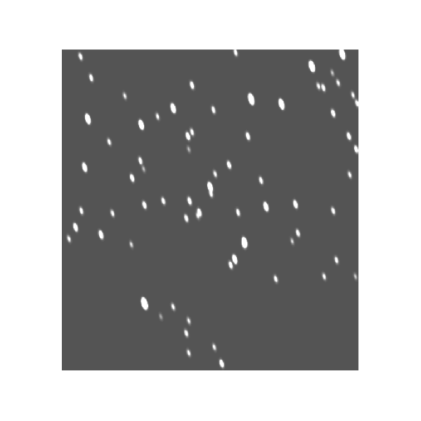
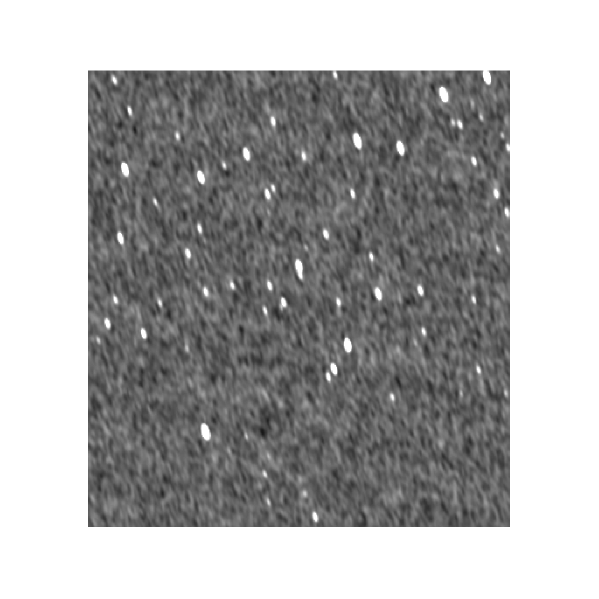
To compare the effectiveness of Sfind 2.0, Imsad and SExtractor, one hundred artificial images $361\times 391$ pixels in size were generated. Each of these contained a different instance of random gaussian noise and the same catalogue of 72 point sources with known properties (position and intensity). The intensity distribution of the sources spans a little more than 2 orders of magnitude, ranging from somewhat fainter than the noise level to well above it. Many fewer bright sources were assigned than faint sources, in order to produce a realistic distribution of source intensities. The artificial images were convolved with a gaussian to mimic the effects of a radio telescope PSF. The test images have $2^{\prime\prime}$ pixels, and the gaussian chosen to represent the PSF has FWHMa of $11\farcs 73\times 5\farcs 52$ with a position angle of $16.3^{\circ}$ . The (convolved) artificial sources in the absence of noise can be seen in Figure 2, along with one of the test images.

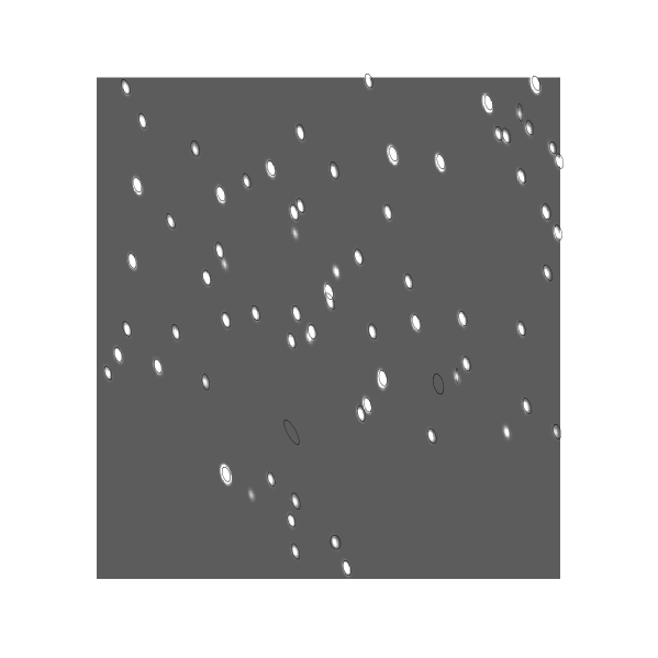
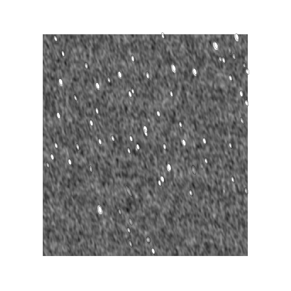
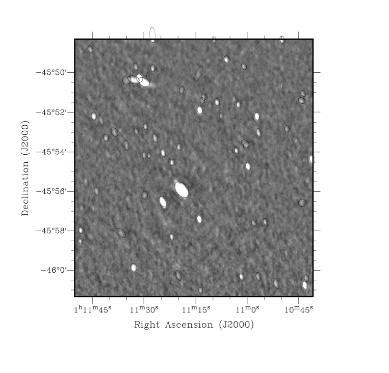
On each image, Sfind 2.0 was run with $\alpha=0.01$ , $0.05$ and $0.1$ , and the resulting lists of detected sources compared with the input catalogue. By way of an example, the sources detected in a single test of Sfind 2.0 are shown in Figure 3, which indicates by an ellipse the location, size and position angle of each detected source. This example demonstrates the difficulty of detecting faint sources, and the ability of noise to mimic the characteristics of faint sources.

3.1 Source pixel detection

Miller et al. (2001) examined the simplest possible scenario, source-pixels placed on a regular grid in the presence of uncorrelated gaussian noise. Here we investigate a much more realistic situation. The ‘source-pixels’ now lie in contiguous groups comprising ‘real’ sources in the sense that the whole image (background and sources) has been convolved with a PSF. The number of pixels in each source above a certain threshold will vary depending on the intensity of the source. We now confirm that the FDR method works consistently on these realistic images.

To verify the reliability of the FDR defined threshold, the number of pixels detected above the FDR threshold in each test were recorded along with the number which were unassociated with any true source. The distribution of this fraction of false FDR pixels should never exceed the value specified for $\alpha$ , and this can be seen in the histogram in Figure 4. This Figure also shows how the distribution of falsely detected pixels changes with the form chosen for $c_{N}$ , emphasising that the assumption of complete independence of the pixels is not justified (as expected), but neither is the image fully correlated, evidenced by the conservative level of false detections seen under this assumption. Our choice for the form of $c_{N}$ , which is not in fact a result of the rigorous statistical proof, appears to be a feasible and reliable intermediate for such ‘partially correlated’ images.

3.2 Source detection

The FDR formalism ensures that the average fraction of falsely detected pixels will be less than $\alpha$ . The connection between numbers of pixels and numbers of sources is complex, however, and the same criterion cannot be said to be true for the fraction of falsely detected sources. The number of source-pixels per source will vary according to both instrumental effects, such as the sampling and the PSF, as well as intrinsic source sizes compared to the instrumental resolution and the source brightnesses compared to the noise level in an image. Even if all sources are point-like, and hence should appear in the image as a PSF, the number of source-pixels above a given threshold for a given source depends on its brightness, and the number of source-pixels per source would not be expected to be constant. To investigate the effect of this complex relation, we explore empirically the results of applying FDR thresholding to our simulated images. The fraction of falsely detected sources in each image, as well as the fraction of true sources not detected, are shown in Figure 5 as distributions for each tested value of $\alpha$ . By construction, a number of the artificial sources have intensities comparable to or lower than the noise level in the images, so not all sources will be able to be recovered in every image. This is reflected in the fact that somewhat more than $5\%$ of sources are missed (by all tasks tested) even with very liberal thresholds.

The histograms in Figure 5(a) show that for $\alpha=0.1$ , where up to $10\%$ of pixels could be expected to be false, the fraction of false sources is not much more. The result for $\alpha=0.05$ , is also quite reasonable, although for $\alpha=0.01$ the outliers are further still, relatively speaking, from the expected fraction. While the strict constraint applicable to the fraction of false source-pixels no longer holds for false sources, it still seems to be quite a good estimator. For the case where only the peak pixel is required to be above the FDR threshold, Figure 5(c), the fractions of falsely detected sources are not so strongly constrained. For $\alpha=0.1$ , the fraction may be almost twice that expected. In both cases, although with greater reliability in the former, this allows the FDR method to provide an estimate of the fraction of false sources to expect. Even though the constraint may not be rigorous, and clearly the estimate will be much more reliable in the case where all source-pixels are required to be above the FDR threshold, the FDR method allows a realistic a priori estimate of the fraction of false detections to be made. This feature is not possible with the simple assumption of, say, a $5\sigma$ threshold.

To test Imsad and SExtractor in the same fashion as Sfind 2.0, a choice of threshold value as a multiple of the image noise level ( $\sigma$ ) was required. Simply selecting a canonical value of $3\sigma$ , $5\sigma$ or $7\sigma$ , for example, would complicate the comparison between these tasks and Sfind 2.0, as this would be testing not only different source measurement routines but also potentially different thresholds. The values of $\alpha$ selected for testing Sfind 2.0 result in threshold levels which correspond approximately, (since the noise level varies minimally from image to image), to $4.1\sigma$ , $3.6\sigma$ and $3.3\sigma$ . A $5\sigma$ threshold in these simulations would correspond to a value of $\alpha\approx 0.0001$ .

In a brief aside, it should be emphasised that this particular correspondence between a choice of $\alpha$ and a particular $\sigma$ -threshold is only valid for the noise and source characteristics of the images used in the present simulations. For images with different noise levels or different source intensity distributions, any particular value of $\alpha$ will correspond to some different multiple of the local noise level. The primary advantage of specifying an FDR $\alpha$ value over choosing a $5\sigma$ threshold, say, is that the FDR threshold is adaptive. The FDR threshold will assume a different value depending on the source intensity distribution relative to the background. This point is made very strongly in Miller et al. (2001) in the diagrams of their Figure 4. As a specific example in the context of the current simulations, we investigated additional simulated images containing the same noise as in the current simulations but containing sources having very different intensity distributions. We chose one intensity distribution such that every source was 10 times brighter than in the current simulations and one such that every source was 10 times fainter. In the brighter case, the FDR threshold for $\alpha=0.01$ , ensuring that on average no more than $1\%$ of source-pixels would be falsely detected, corresponded not to $4.1\sigma$ , but to about $3.8\sigma$ . The reason here is that as the source distribution becomes brighter, many more pixels will have low $p$ -values. To retain the constant fraction of false pixels more background pixels must be included, so the threshold becomes lower. In the fainter case, where the artificial sources are very close in intensity to the noise level, the same FDR threshold corresponds to about $4.4\sigma$ . Of course in this case very few sources are detected, for obvious reasons, but the same constraint on the fraction of falsely detected pixels applies. Here fewer pixels will have low $p$ -values, thus fewer background pixels are allowed, maintaining a constant fraction of false pixels, and the threshold increases. In the brighter case the simple assumption of, say, a $4\sigma$ threshold would give a lower rate of false pixels, while in the fainter case it would give a higher fraction. The importance of these examples is to emphasise that FDR provides a consistent constraint on the fraction of false detections in an adaptive way, governed by the source intensity distribution relative to the background, which cannot be reproduced by the simple assumption of, for example, a $4\sigma$ threshold. While the source distributions in most astronomical images typically lie between the two extremes presented for this illustration, the adaptability of the FDR thresholding method still presents itself as an important tool.

Returning now to the comparison between Sfind 2.0, Imsad and SExtractor, the Imsad and SExtractor thresholds were set to correspond to those derived from the $\alpha$ values used in Sfind 2.0. The distributions of falsely detected and missed sources were similarly calculated. These are shown in Figures 5(e) to 5(h). One of the features of SExtractor is the ability to set a minimum number of contiguous pixels required before a source is considered to be real, and obviously the number of detected sources varies strongly with this parameter. After some experimentation we set this parameter to 7 pixels, as this resulted in a distribution of false detections most similar to that seen with Sfind 2.0, for the case where only pixels above the FDR threshold are used in source measurements. Values larger than 7 reduced the number of false detections at the expense of missing more true sources, and vice-versa. From this comparison, Sfind 2.0 appears to miss somewhat fewer of the true sources than SExtractor when SExtractor is constrained to the same level of false detections. This is also true if SExtractor is constrained to a similar distribution of false detections as obtained by Sfind 2.0 for the case where only the peak pixel is required to be above the FDR threshold (corresponding to 4 contiguous pixels). In both cases, allowing SExtractor to detect more true sources by lowering the minimum pixel criterion introduces larger numbers of false detections. Sfind 2.0 also performs favourably compared to Imsad. While Sfind 2.0 seems to miss a few percent more real sources than Imsad, Imsad seems to detect many more false sources than Sfind 2.0 in either of its source-measurement modes.

Of primary importance in source measurement is the reliability of the source parameters measured. Figure 6 shows one example from the one hundred tests comparing the true intensities and positions of the artificial sources with those measured by Sfind 2.0. Similar results are obtained with Imsad, which uses the same gaussian fitting routine. As expected, the measured values of intensity and position become less reliable as the source intensity becomes closer to the noise, although they are still not unreasonable. A comprehensive analysis of gaussian fitting in astronomical applications has been presented by Condon (1997), and the results of the gaussian fitting performed by Sfind 2.0 (and Imsad) are consistent with the errors expected. Additionally, the assumption that a source is point-like, or only slightly extended, and thus well fit by a two-dimensional elliptical gaussian, is clearly not always true. Complex sources in radio images, as in any astronomical image, present difficulties for simple source detection algorithms such as the ones investigated here. It is not the aim of the current analysis to address these problems, except to mention that the parameters of such sources measured under the point-source assumption will suffer from much larger errors than indicated by the results of the gaussian fitting.

As a final test, Sfind 2.0 was used to identify sources in a real radio image, a small portion of the Phoenix Deep Survey (Hopkins et al., 1999). This image contains sources with extended and complex morphologies as well as point sources. Figure 7 shows the results, with Sfind 2.0 reliably identifying point source and extended objects as well as the components of various blended sources and complex objects.

4 Discussion

The main aims of this analysis have been to (1) investigate the implementation of FDR thresholding to an astronomical source detection task, and (2) compare the rates of missed and falsely detected sources between this task and others commonly used. Implementation of the FDR thresholding method is very straightforward, (evidenced by the seven step IDL example of Miller et al. (2001), in their appendix B). The FDR method performs as expected in providing a statistically reliable estimate of the fraction of falsely detected pixels. Performing source detection on a set of pixels introduces the transformation of pixel groups into sources. This ultimately results in the strong constraint on the false fraction of FDR-selected pixels becoming a less rigorous, but still useful and reliable estimate of the fraction of false sources. As already mentioned, this is still a more quantitative statement than can be made of the rate of false sources in the absence of the FDR method. It is possible that rigorous quantitative constraints on the fraction of false source detections may be obtained empirically for individual images or surveys. By performing Monte-Carlo source detection simulations with artificial images having noise properties similar to the ones under investigation, the trend of falsely detected sources with $\alpha$ may be able to be reliably characterised. This has not been examined in the current analysis, but will be included in subsequent work with Sfind 2.0. While constraints on the fraction of falsely detected sources may be possible, neither FDR nor any other thresholding method provides constraints on the numbers of true sources remaining undetected.

A study is also ongoing into whether a more sophisticated FDR thresholding method for defining a source may be feasible. This would involve examining the combined size and brightness properties of groups of contiguous pixels to define a new $p$ -value. This would represent the likelihood that such a collection of pixels comes from a ‘background distribution’ or null-hypothesis, corresponding to the properties exhibited by noise in various types of astronomical images. Using this new $p$ -value an FDR threshold, now in the size-brightness parameter space, could be applied for defining a source catalogue. Clearly much care will need to be taken to avoid discriminating against true sources which may lie in certain regions of the size-brightness plane, such as low surface-brightness galaxies. The assumption in many existing source-detection algorithms that sources are point-like already suffers from such discrimination, though, so even if such bias is unavoidable, some progress may still be achievable.

The form assumed for $c_{N}$ in this analysis is not in fact a rigorous result of the formal FDR proof. Instead it is a ‘compromise’ estimate that seems mathematically reasonable, and gives reliable results in practice. To be strictly conservative, the form of $c_{N}$ given by equation 1 should be adopted to ensure that the fraction of falsely detected ‘source-pixels’ is strictly less than $\alpha$ . This rigorous treatment, however, is dependent on the number of pixels present in the image. Now consider analysis of a sub-region within an image. As the size of this sub-region is changed, the number of pixels being considered similarly changes, and this will have the effect of changing the threshold level, and the resulting source catalogue. This, perhaps non-intuitive, aspect of the FDR formalism is the adaptive mechanism which allows it to be rigorous in constraining the fraction of false detections.

There are additional complicating factors which must be taken into account when performing source detection. The null hypothesis assumed for the FDR method (and indeed for all the source detection algorithms) is that the background pixels have intensities drawn from a gaussian distribution (or other well-characterised statistical distribution such as a poissonian). This is not strictly true for radio images, where residual image processing artifacts may affect the noise properties, albeit at a low level. In all cases, such deviations will result in a larger fraction of false pixels than expected, some of which may be clumped in a fashion sufficient to mimic, and be measured as, sources, thus increasing the fraction of falsely detected sources. This comment is simply to serve as reminder to use caution when analysing images with complex noise properties.

5 Conclusions

We have implemented the FDR method in an astronomical source detection task, Sfind 2.0, and compared it with two other tasks for detecting and measuring sources in radio telescope images. Sfind 2.0 compares favourably to both in the fractions of falsely detected sources and undetected true sources. The FDR method reliably selects a threshold which constrains the fraction of false pixels with respect to the total number of ‘source-pixels’ in realistic images. The fraction of falsely detected sources is not so strongly constrained, although quantitative estimates of this fraction are still reasonable. More investigation of the relationship between ‘source-pixels’ and ‘sources’ is warranted to determine if a more rigorous constraint can be established. With the ability to quantify the fraction of false detections provided by the FDR method, we strongly recommend that it is worthwhile implementing as a threshold defining method in existing source detection tasks.

We would like to thank the referee for several suggestions which have improved this paper. AMH acknowledges support provided by NASA through Hubble Fellowship grant HST-HF-01140.01-A awarded by the Space Telescope Science Institute (STScI). AMH and AJC acknowledge support provided by NASA through grant numbers GO-07871.02-96A and NRA-98-03-LTSA-039 from STScI, and AISR grant NAG-5-9399. STScI is operated by the Association of Universities for Research in Astronomy, Inc., under NASA contract NAS5-26555.

References

Benjamini & Hochberg (1995) Benjamini, Y., Hochberg, Y. 1995, J. R. Stat. Soc. B, 57, 289
Benjamini & Yekutieli (2001) Benjamini, Y., Yekutieli, D. 2001, Ann. Statist., (in press)
Bertin & Arnouts (1996) Bertin, E., Arnouts, S. 1996, A&AS, 117, 393
Condon (1997) Condon, J. J. 1997, PASP, 109, 166
Hopkins et al. (1999) Hopkins, A., Afonso, J., Cram, L., Mobasher, B. 1999, ApJ, 519, L59
Miller et al. (2001) Miller, C. J., Genovese, C., Nichol, R., Wasserman, L., Connolly, A., Reichart, D., Hopkins, A., Schneider, J., Moore, A. 2001, AJ (accepted) (astro-ph/0107034)
White et al. (1997) White, R. L., Becker, R. H., Helfand, D. J., Gregg, M. D., 1997, ApJ, 475, 479

Refer to caption — Figure 1: A graphical example of how the FDR threshold is calculated. This diagram shows only the relevant portion of the full graph (which has abscissa spanning $0-1$ ). The points show $p$ -values of the pixels from one of the artificial images. The line has a slope of $\alpha/c_{N}$ with $\alpha=0.05$ and $c_{N}\approx 3.495$ , corresponding to a PSF area covering 18 pixels. The last intersection point gives $p_{\rm cut}=2.19\times 10^{-4}$ . Hence all pixels with $p<2.19\times 10^{-4}$ are considered ‘source-pixels’.