Abstract

The “core” of a radio source is believed to mark the frequency-dependent location where the optical depth to synchrotron self–absorption $\tau_{s}\approx 1$. The frequency dependence can be used for derive physical conditions of the radio emitting region and the ambient environment near the central engine of the radio source. In order to test and improve the models to derive this information, we made multi-frequency dual-polarization observations of 3C 309.1 in 1998.6, phase-referenced to the QSOs S5 1448+76 and 4C 72.20 (S5 1520+72) ($4^{\circ}26^{\prime}$ and $1^{\circ}49^{\prime}$ away, respectively). We present here preliminary results from these observations: total and polarized intensity maps, spectral information deduced from these images, and the relative position of 3C 309.1 with respect to S5 1448+76 at different frequencies. Finally, we discuss briefly the observed shift of the core position.

1 Introduction

Opacity in pc-scale jets

The unresolved “core” of a compact extragalactic radio source is believed to mark the location where the optical depth to synchrotron self absorption $\tau_{s}\approx 1$. This position changes with observing frequency as $R_{\rm core}\propto\nu^{-1/k_{r}}$ [1]. The power index $k_{r}$ depends on the shape of the electron energy spectrum and on the magnetic field and particle density distributions in the ultra-compact jet. Hence, by studying variations at $k_{r}$ as a function of frequency, we may study the detailed physical conditions of the radio emitting region and the ambient environment of the source very near the central engine. Following [2] we can estimate basic physical parameters of the jet including luminosity, maximum brightness temperature, magnetic field in the jet, particle density, and the geometrical properties of the jet (i.e., the core location respect to the jet origin).

To measure $k_{r}$ a knowledge of the absolute position of the core (or at least the core offset between different frequencies) is needed. Hybrid maps in VLBI lack this positional information due to the use of closure-phase in the imaging process. The rigorous alignment of hybrid maps can be made by astrometric phase-referencing (e.g. [3, 4, 5, 6]). In sources with extended structure, an optically thin component can be used to align maps at different frequencies and then estimate the position of the core.

The QSO 3C 309.1

The QSO 3C 309.1 (V$=$16.78, $z$=0.905) is one of the most prominent compact steep spectrum (CSS) radio sources [7, 8]. Many of the CSS sources display polarized emission at cm-wavelengths. The ionized gas surrounding the jet disrupts its flow and is responsible of the complexity of the radio structures seen. There is evidence suggesting that 3C 309.1 is located at the center of a very massive cooling flow with $\dot{M}>1000\,{\rm M}_{\odot}\,{\rm yr}^{-1}$ within a radius of 11.5 h^-1 kpc [9].

VLBA observations of 3C 309.1 at 6 frequencies were used for determining the behavior of $k_{r}$ between 1.6 and 22 GHz [2]. To improve and extend this determination to higher frequencies, we observed 3C 309.1 using the VLBA at eight frequencies with dual polarization. In this contribution, we present a preliminary analysis of the new observations.

2 Mapping analysis

VLBA Observations

We carried out VLBA multi-frequency, dual-polarization observations of 3C 309.1 on July 19th and 23rd 1998 using all 10 VLBA antennas and observing at 1.5, 1.6, 2.3, 5, 8.4, 15, 22, and 43 GHz. The data were correlated at the NRAO and processed using aips and difmap [13]. difmap was used for mapping the total intensity emission. The polarized intensity mapping and the phase-referencing analysis were carried out in aips. The 43 GHz data had to be discarded due to calibration and coherence problems.

Total intensity mapping

We applied the clean algorithm and self-calibration in difmap to obtain the total intensity maps presented in Fig. 1 and described in Table 1. The resulting images show a structure very similar to the reported in earlier works (see [10] and references therein). The source shows a core-jet structure first oriented southward and turning later to the East at about 60 mas from the core.

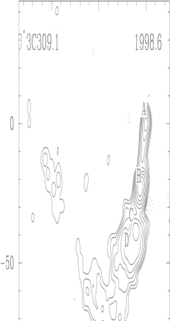
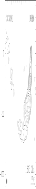
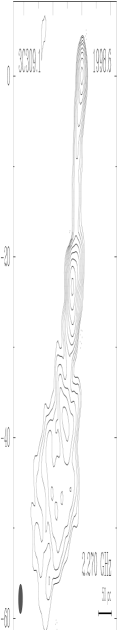
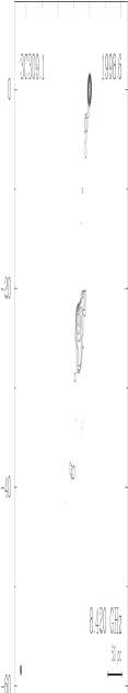
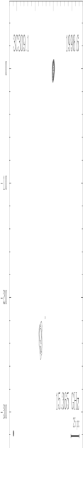
Figure 1: VLBA total intensity images of 3C 309.1. The synthesized interferometric beams are represented at the bottom left corner of each image. Contour levels are drawn at $\sqrt{2}$ intervals. The left image follows the labelling convention from [12]. Map parameters (beam, total flux density, peak of brightness, lowest contour in map) are given in Table 1.

Table 1: Total intensity map parameters (Figs. 1 & 4)

	— 3C 309.1 —						— 4C 72.20 —						— S5 1448+76 —
	Beam						Beam						Beam
$\nu$	size		P.A.	$S_{\rm peak}$	$S_{\rm min}$(a)	$S_{\rm tot}$(b)	size		P.A.	$S_{\rm peak}$	$S_{\rm min}$(a)	$S_{\rm tot}$(b)	size		P.A.	$S_{\rm peak}$	$S_{\rm min}$(a)	$S_{\rm tot}$(b)
[Hz]	[mas]		[∘]	[Jy/b]	[mJy/b]	[Jy]	[mas]		[∘]	[Jy/b]	[mJy/b]	[Jy]	[mas]		[∘]	[Jy/b]	[mJy/b]	[Jy]
1.505	5.00$\times$	4.60	–7.5	0.972c	2.0	3.424	6.47$\times$	5.96	–5.5	0.053	0.5	0.055	6.49$\times$	6.21	1.7	0.145	0.6	0.171
1.675	4.50$\times$	4.10	–4.3	0.819c	2.0	3.181	5.83$\times$	5.34	–4.5	0.050	0.4	0.052	5.77$\times$	5.50	–3.3	0.149	0.6	0.174
2.270	3.19$\times$	2.90	–10.5	0.604c	2.0	2.699	4.09$\times$	3.68	–8.4	0.083	0.8	0.085	4.11$\times$	3.74	–13.8	0.225	0.8	0.253
4.987	1.40$\times$	1.35	8.5	0.675d	2.0	1.797	1.90$\times$	1.82	–13.6	0.053	0.4	0.065	1.88$\times$	1.79	–24.8	0.263	0.6	0.313
8.420	0.95$\times$	0.85	–5.0	0.646d	2.0	1.326	1.08$\times$	0.99	–6.7	0.056	0.8	0.057	1.10$\times$	1.02	–11.0	0.216	0.8	0.303
15.365	0.47$\times$	0.45	–17.8	0.492d	3.0	0.921	0.58$\times$	0.56	–14.8	0.100	0.8	0.101	0.59$\times$	0.58	4.7	0.156	1.1	0.244
22.233	0.41$\times$	0.33	–14.8	0.430d	3.0	0.712	0.54$\times$	0.45	–0.2	0.195	1.5	0.205	0.55$\times$	0.45	–6.6	0.211	1.6	0.241

^a Minimum contour level in the figure. ^b Total flux density recovered in the map model. ^c Corresponds to the B component. ^d Corresponds to the A component.

Polarized intensity maps

We applied the instrumental polarization calibration from the total intensity maps using the aips task lpcal as described in [14]. We imaged the Stokes Q and U and produced images of the linearly polarized emission and the electric vector position angle. An exhaustive description of these results will be published elsewhere. We show an image of the linear polarization distribution at 1.5 GHz in Fig. 2. The core is unpolarized as in many QSOs. In the region South of B the electric vector is radial, suggesting a toroidal magnetic field viewed edge-on. The degree of polarization is higher at the outer parts of the jet.

Figure 2: Polarized intensity image of 3C 309.1 at 1.505 GHz ($\lambda$ 21cm). Electric field vectors are shown.

Spectral analysis

The overall spectral index of 3C309.1 is $-0.57\pm 0.01$. This result is obtained by adding together emission from all of the radio source structure which may have very different physical properties.

To study spectral properties at different parts of the source, we mapped the radio source at all frequencies using natural weighting and very strong tapering (Gaussian function with half maximum at a distance of 33 M$\lambda$). We convolved the clean components with a circular beam of 4 mas in size, aligning the images on the peak-of-brightness of component A. We show these images in Fig. 3 together with the spectra of components A and B and the total spectrum of the VLBI emission. The turnover frequency for A is around 8.4 GHz, and is below 1.4 GHz for B. A linear regression to the points for B provides an overall spectral index of $-0.67\pm 0.04$.

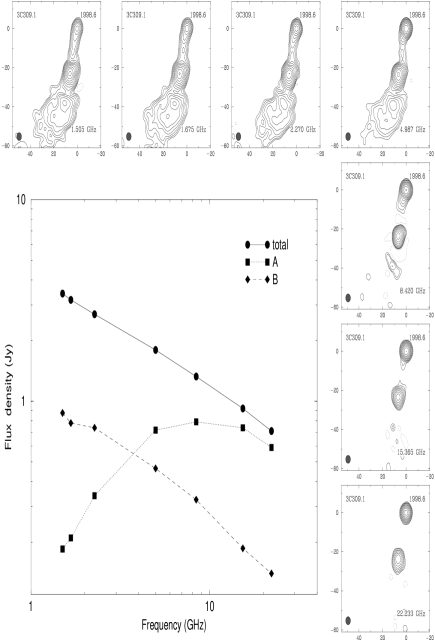
Figure 3: Maps of 3C 309.1 at 4 mas resolution, obtained using the natural weighting and Gaussian tapering with the half maximum at 33 M$\lambda$. The contour levels are drawn at $\sqrt{3}$ intervals. The lowest level is of 3 mJy/beam

3 Phase-referencing analysis

The calibrators

We used two position calibrators for 3C 309.1:

• 4C 72.20 is a QSO with $z$=$0.799$ and $V$=$16.5$, $1^{\circ}49^{\prime}$ East of the target source. It is a point-like source with an inverted spectrum. The imaging results are presented in Fig. 4.

• S5 1448+76 is a flat spectrum, compact radio source with $z$=$0.899$ and $V$=$20.0$. It is $4^{\circ}26^{\prime}$ to the NW of 3C 309.1. It shows a faint jet to the NE at the lower frequencies, and it is also elongated in the East-West direction at the higher frequencies. The hybrid maps are shown in Fig. 4.

Figure 4: Hybrid maps of the position calibrator sources 4C 72.20 (top) and S5 1448+76 (bottom). The map parameters are described in Table 1.

The analysis

We carried out the phase-referencing analysis in aips. We solved for the phase, delay and phase-rate for 3C 309.1, using the total intensity maps as input (dividing the $(u,v)$-data by the clean model) and thus removing the effect of the source structure. We then interpolated the values fitted using the task clcal for the fainter phase-reference calibrators, S5 1442+76 and 4C 72.20 (S5 1520+76).

After editing the data, we mapped the radio sources using the aips task imagr with the same parameters as were used for the hybrid imaging in difmap. The phase-referenced maps are shown in Fig. 5 and the corresponding map parameters are given in Table 2. We measured the positions of the brightness peaks, whose offsets from the coordinate origin correspond to the offsets from the nominal position of 3C 309.1 relative to the calibrators. The relative positions deduced from this procedure are presented in Table 3.

Figure 5: Phase-reference maps of 4C 72.20 and S5 1448+76 obtained using the phase, delay and phase-rate solutions for 3C 309.1 as described in the text. The contours are 49, 69 and 98% of the peak of brightness for each map. The values of the brightness peaks and their ratio (in percentage) with respect to their peaks in the hybrid maps (Fig. 4) are given in Table 2.

Table 2: Phase-referenced map parameters for 4C 72.20 and S5 1448+76 (Fig. 5)

	— 4C 72.20 —			— S5 1448+76 —
$\nu$	$S_{\rm max}^{\phi{\rm-ref}}$	$S_{\rm max}^{\rm hybrid}$	$\frac{S_{\rm max}^{\phi{\rm-ref}}}{S_{\rm max}^{\rm hybrid}}$	$S_{\rm max}^{\phi{\rm-ref}}$	$S_{\rm max}^{\rm hybrid}$	$\frac{S_{\rm max}^{\phi{\rm-ref}}}{S_{\rm max}^{\rm hybrid}}$
[GHz]	[mJy/beam]	[mJy/beam]	[%]	[mJy/beam]	[mJy/beam]	[%]
1.505	13.6	53.3	25.5	29.2	145.2	20.1
1.675	14.8	49.7	29.8	33.3	148.7	22.4
2.270	30.0	82.3	36.5	82.4	225.3	36.6
4.987	19.0	52.8	36.0	143.7	263.2	54.6
8.420	7.1	55.3	12.8	55.3	216.3	25.6
15.365	4.7	100.4	4.7	22.2	155.8	14.2
22.233	—			11.9	211.3	5.6

Table 3: Relative right ascensions and declinations in J2000.0 coordinates of 3C 309.1 with respect to 4C 72.20, and S5 1448+76, obtained via aips phase-referencing. Biases have not been corrected.

— 4C 72.20 —

— S5 1448+76 —

$\nu$ [GHz]

$\Delta\alpha_{({\rm 3C\,309.1~{}-~{}4C\,72.20})}$

$\Delta\delta_{({\rm 3C\,309.1~{}-~{}4C\,72.20})}$

$\Delta\alpha_{({\rm 3C\,309.1~{}-~{}S5\,1448+76})}$

$\Delta\delta_{({\rm 3C\,309.1~{}-~{}S5\,1448+76})}$

1.505

–0h

21m

40$\hbox to0.0pt{.\hss}^{\rm s}$

0554 $\pm$

0$\hbox to0.0pt{.\hss}^{\rm s}$

0015

–0∘

44′

45$\hbox to0.0pt{.\hss}^{\prime\prime}$

712 $\pm$

0$\hbox to0.0pt{.\hss}^{\prime\prime}$

007

0h

10m

38$\hbox to0.0pt{.\hss}^{\rm s}$

805 $\pm$

0$\hbox to0.0pt{.\hss}^{\rm s}$

002

–4∘

20′

51$\hbox to0.0pt{.\hss}^{\prime\prime}$

721 $\pm$

0$\hbox to0.0pt{.\hss}^{\prime\prime}$

006

1.675

–0h

21m

40$\hbox to0.0pt{.\hss}^{\rm s}$

0557 $\pm$

0$\hbox to0.0pt{.\hss}^{\rm s}$

0015

–0∘

44′

45$\hbox to0.0pt{.\hss}^{\prime\prime}$

712 $\pm$

0$\hbox to0.0pt{.\hss}^{\prime\prime}$

007

0h

10m

38$\hbox to0.0pt{.\hss}^{\rm s}$

8045 $\pm$

0$\hbox to0.0pt{.\hss}^{\rm s}$

0014

–4∘

20′

51$\hbox to0.0pt{.\hss}^{\prime\prime}$

722 $\pm$

0$\hbox to0.0pt{.\hss}^{\prime\prime}$

005

2.270

–0h

21m

40$\hbox to0.0pt{.\hss}^{\rm s}$

0568 $\pm$

0$\hbox to0.0pt{.\hss}^{\rm s}$

0014

–0∘

44′

45$\hbox to0.0pt{.\hss}^{\prime\prime}$

708 $\pm$

0$\hbox to0.0pt{.\hss}^{\prime\prime}$

006

0h

10m

38$\hbox to0.0pt{.\hss}^{\rm s}$

8053 $\pm$

0$\hbox to0.0pt{.\hss}^{\rm s}$

0007

–4∘

20′

51$\hbox to0.0pt{.\hss}^{\prime\prime}$

726 $\pm$

0$\hbox to0.0pt{.\hss}^{\prime\prime}$

003

4.987

–0h

21m

40$\hbox to0.0pt{.\hss}^{\rm s}$

0565 $\pm$

0$\hbox to0.0pt{.\hss}^{\rm s}$

0014

–0∘

44′

45$\hbox to0.0pt{.\hss}^{\prime\prime}$

707 $\pm$

0$\hbox to0.0pt{.\hss}^{\prime\prime}$

006

0h

10m

30$\hbox to0.0pt{.\hss}^{\rm s}$

80476 $\pm$

0$\hbox to0.0pt{.\hss}^{\rm s}$

00017

–4∘

20′

51$\hbox to0.0pt{.\hss}^{\prime\prime}$

7313 $\pm$

0$\hbox to0.0pt{.\hss}^{\prime\prime}$

0006

8.420

–0h

21m

40$\hbox to0.0pt{.\hss}^{\rm s}$

0569 $\pm$

0$\hbox to0.0pt{.\hss}^{\rm s}$

0014

–0∘

44′

45$\hbox to0.0pt{.\hss}^{\prime\prime}$

706 $\pm$

0$\hbox to0.0pt{.\hss}^{\prime\prime}$

006

0h

10m

30$\hbox to0.0pt{.\hss}^{\rm s}$

80482 $\pm$

0$\hbox to0.0pt{.\hss}^{\rm s}$

00009

–4∘

20′

51$\hbox to0.0pt{.\hss}^{\prime\prime}$

7320 $\pm$

0$\hbox to0.0pt{.\hss}^{\prime\prime}$

0003

15.365

–0h

21m

40$\hbox to0.0pt{.\hss}^{\rm s}$

0568 $\pm$

0$\hbox to0.0pt{.\hss}^{\rm s}$

0014

–0∘

44′

45$\hbox to0.0pt{.\hss}^{\prime\prime}$

705 $\pm$

0$\hbox to0.0pt{.\hss}^{\prime\prime}$

006

0h

10m

30$\hbox to0.0pt{.\hss}^{\rm s}$

80489 $\pm$

0$\hbox to0.0pt{.\hss}^{\rm s}$

00008

–4∘

20′

51$\hbox to0.0pt{.\hss}^{\prime\prime}$

7318 $\pm$

0$\hbox to0.0pt{.\hss}^{\prime\prime}$

0003

22.233

—(a)

—(a)

0h

10m

30$\hbox to0.0pt{.\hss}^{\rm s}$

80482 $\pm$

0$\hbox to0.0pt{.\hss}^{\rm s}$

00007

–4∘

20′

51$\hbox to0.0pt{.\hss}^{\prime\prime}$

7315 $\pm$

0$\hbox to0.0pt{.\hss}^{\prime\prime}$

0003

^a No phase-referencing detection.

The catalogue position of 4C 72.20 used at the correlator in error of +200 in $\alpha$ and –280 mas in $\delta$. This translates into an estimated uncertainty of $\sim$6 mas, in our preliminary position determination at each frequency, making this fraction of the data unusable for our purposes. A proper analysis, correcting for the wrong position of 4C 72.20 will be published elsewhere. No ionosphere corrections have been applied in the data analysis. At frequencies lower than 8.4 GHz, the ionospheric dispersion may severely bias our results. The tropospheric delay, especially the wet part, affects the phase for the highest frequencies, where the size of the water particles in the atmosphere is comparable to the wavelength.

Notice that the ratio between the peaks of brightness of the phase-referenced maps and the hybrid maps (4^th and 7^th columns in Table 2) is the highest at the intermediate frequencies, where the compromise between the ionospheric and the tropospheric effects is found. Even when the a priori position of 4C 72.20 is in error, its ratios are similar to the ones in S5 1448+76, probably because the former is $\sim$3 times closer to 3C 309.1 than the latter.

The error budget in the positions (uncertainties in Table 3) includes the following error terms: a priori coordinates of the source, determination of peak-of-brightness in the maps, polar motion (estimated error of 1 mas), UT1–UTC (10^-4s), station coordinates (5 cm), troposphere, ionosphere ($\propto\nu^{-2}$), and problems in the aips phase connection. This constitutes a conservative estimate of the uncertainty. We consider thus the phase-referencing results with S5 1448+76 at the highest frequencies as correct (central panel of Fig. 6).

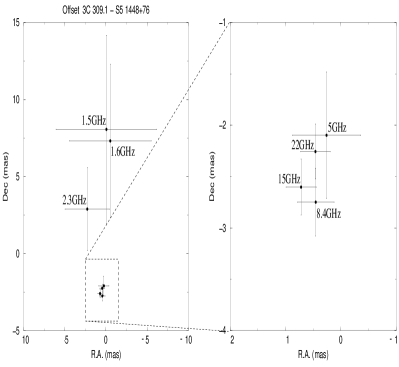
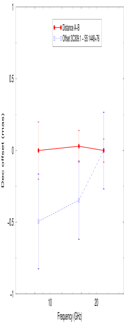
Figure 6: Left and central panel: Relative position of 3C 309.1 with respect to S5 1448+76, obtained via aips phase-referencing as described in the text. The data at the lowest frequencies are dominated by the ionospheric effect and are invalid for our purposes. Right panel: Comparison between the two different methods presented in the text to determine the core offset at 8.4, 15 and 22 GHz: the distance A-B with respect to the phase referencing results. The values at 22 GHz are set as zero reference. The A-B offset is biased due to beam effects in the L-shaped B component. The astrometric results are biased by the unmodelled ionosphere and a simplistic model for the troposphere.

The core position

We assign the peak offset in $\alpha$ to S5 1448+76 and in $\delta$ to 3C 309.1. The declination offsets in 3C 309.1 between contiguous frequencies are shown in Table 4. The relative offsets are also plotted in Fig. 6, where the value at 22 GHz has been set to be zero.

Table 4: Core shift in declination for 3C 309.1 at the higher frequencies (see right panel in Fig. 6).

	Distance A-B	aips phase-
Frequencies	in maps	referencing
15 – 8.4 GHz	–130$\pm$140 $\mu$as	150$\pm$430 $\mu$as
22 – 15 GHz	130$\pm$140 $\mu$as	350$\pm$380 $\mu$as

An alternative way to measure the core offset is to assume that the B component in the maps from Section 2 is optically thin and its peak is at the same position for all frequencies. These values are also presented in Table 4, and in the right panel of Fig. 6.

The trend in the dependence of the core position with the frequency is different in both methods. The A–B separation measurements is apparently frequency-independent: the difference at the beams at different frequencies may bias this result, since the structure of the B component is L-shaped and in the declination coordinate it is more extended to the South. Our preliminary positional results from the aips astrometry at 8.4, 15 and 22 GHz (but not at 5 GHz) suggest that the peak-of-brigthness of the maps shifts closer to the jet basis (core at infinite frequency) at higher frequencies, being this jet basis to the North of the A feature. This would be the expected opacity shift produced by the synchrotron self-absorption in the jet. Assuming that $k_{r}$=1 (self-absorbed core, [15]) at 8.4 GHz and that $R_{\rm core}\propto\nu^{-1/k_{r}}$, the astrometric results provide values of $k_{r}$=1.1$\pm$0.5 at 15 GHz and $k_{r}$=0.9$\pm$0.6 at 22 GHz. The big uncertainties do not permit to draw any conclusions about the physical parameters of the jet from $k_{r}$ at the present status of the analysis. A detailed analysis with the final, unbiased astrometric results will be published elsewhere.

4 Summary

We have presented preliminary results from a detailed multi-frequency study of the QSO 3C 309.1 based on the VLBA observations made in mid 1998. We find a curved jet extending up to 100 mas to the East at low frequencies with two main components, A and B. The A component has a turnover frequency around 8.4 GHz and the B component is optically thin. The polarized intensity map at 1.5 GHz shows that the core is un polarized. In the region southern to B the electric field has a radial structure. The external parts of the jet have a high degree of polarization. A preliminary astrometric analysis provides a determination of the core position at different frequencies by phase-referencing to a nearby radio source QSO S5 1448+76. The changes at the core position with frequency suggest high opacity close to the core caused by synchrotron self-absorption. Due to the big uncertainties we cannot make any assert about the value of $k_{r}$ at high frequencies. An exhaustive analysis including ionospheric and tropospheric bias removal and physical modeling of the source will be presented in a forthcoming paper.

Acknowledgements. We acknowledge Dr. Scott E. Aaron for his support during the data collection and Dr. Richard W. Porcas for his critical reading of the manuscript. The National Radio Astronomy Observatory is a facility of the National Science Foundation operated under cooperative agreement by Associated Universities, Inc.

References

- [1] Königl, A. 1981, AJ 243, 700
- [2] Lobanov, A. P. 1998, A&A 330, 79
- [3] Lebach, D. E., Ransom, R. R., Ratner, M. I., Shapiro, I. I., Bartel, N., Bietenholz, M. F., Lestrade, J.-F., 2001, in ”Galaxies and their Constituents at the Highest Angular Resolution”, IAU Symp. 205, p. 59
- [4] Brisken, W. F., Benson, J. M., Beasley, A. J., Fomalont, E. B., Goss, W. M., Thorsett, S. E., 2000, ApJ 541, 959
- [5] Pérez-Torres, M. A., Marcaide, J. M., Guirado, J. C., Ros, E., Shapiro, I. I., Ratner, M. I., Sardón, E., 2000, A&A 360, 161
- [6] Ros, E., Marcaide, J. M., Guirado, J. C., Ratner, M. I., Shapiro, I. I., Krichbaum, T. P., Witzel, A., Preston, R. A., 1999, A&A 348, 381
- [7] van Breugel, W., Miley, G., Heckman, T., 1984, AJ 89, 5
- [8] Fanti, C., Fanti, R., Parma, P., Schilizzi, R. T., van Breugel, W. J. M. 1985, A&A 143, 292
- [9] Forbes, D. A., Crawford, C. S., Fabian, A. C., Johnstone, R. M. 1990, MNRAS 244, 680
- [10] Aaron. S. E., 1996, PhD Thesis, Brandeis University, MA, US
- [11] Aaron, S. E., Wardle, J. F. C., Roberts, D. H. 1997, Vistas in Astronomy 41, 225
- [12] Kus, A. J., Wilkinson, P. N., Pearson, T. J., Readhead, A. C. S. 1990, in: Parsec-Scale Radio Jets, ed. J.A. Zensus, T.J. Pearson, Cambridge University Press, 161
- [13] Shepherd, M. C., Pearson, T. J., Taylor, G. B. 1995, BAAS 26, 987
- [14] Leppänen, K. J., Zensus, J. A., Diamond, P. J. 1995, AJ 100, 2479
- [15] Blandford, R. D., Königl, A. 1979, ApJ 232, 34