Reliability of astrophysical jet simulations in 2D

In the present paper, we examine the convergence behavior and inter-code reliability of astrophysical jet simulations in axial symmetry. We consider both pure hydrodynamic jets and jets with a dynamically significant magnetic field. The setups were chosen to match the setups of two other publications, and recomputed with the MHD code NIRVANA. We show that NIRVANA and the two other codes give comparable, but not identical results. We explain the differences by the different application of artificial viscosity in the three codes and numerical details, which can be summarized in a resolution effect, in the case without magnetic field: NIRVANA turns out to be a fair code of medium efficiency. It needs approximately twice the resolution as the code by Lind (Lind et al. 1989) and half the resolution as the code by Kössl (Kössl & Müller 1988). We find that some global properties of a hydrodynamical jet simulation, like e.g. the bow shock velocity, converge at 100 points per beam radius (ppb) with NIRVANA. The situation is quite different after switching on the toroidal magnetic field: In this case, global properties converge even at 10 ppb. In both cases, details of the inner jet structure and especially the terminal shock region are still insufficiently resolved, even at our highest resolution of 70 ppb in the magnetized case and 400 ppb for the pure hydrodynamic jet. The magnetized jet even suffers from a fatal retreat of the Mach disk towards the inflow boundary, which indicates that this simulation does not converge, in the end. This is also in definite disagreement with earlier simulations, and challenges further studies of the problem with other codes. In the case of our highest resolution simulation, we can report two new features: First, small scale Kelvin-Helmholtz instabilities are excited at the contact discontinuity next to the jet head. This slows down the development of the long wavelength Kelvin-Helmholtz instability and its turbulent cascade to smaller wavelengths. Second, the jet head develops Rayleigh-Taylor instabilities which manage to entrain an increasing amount of mass from the ambient medium with resolution. This region extends in our highest resolution simulation over 2 jet radii in the axial direction.

1 Introduction

Since the publication of the “twin exhaust model” (Blandford & Rees (1974)), astrophysical jets have been modeled by many workers. These jets consist of a highly collimated outflow of magnetized plasma from a compact object, which – in the case of extragalactic jets – is assumed to be a black hole, and its accretion disk. In order to study the asymptotic propagation of such a plasma flow one needs a code that solves the equations of (magneto-) hydrodynamics (MHD/HD) for the relevant initial and boundary conditions. Pioneers in this field were M. L. Norman and coworkers in 1982 (Norman et al. (1982)). They were able to show that a flow of supersonic plasma remains stable and develops features that could be identified with features in the observations of radio galaxies: A circular or conical deceleration area called Mach disk as the hot spot, a strongly collimated beam as the elongated structure of the jets, and a big zone of exhaust material as the lobes of the radio galaxies (see also Ferrari (1998) for a recent review). Meanwhile, more physics has been included in the calculations such as toroidal (perpendicular to the jet flow direction and the jet radius) magnetic fields (Clarke et al. (1986); Lind et al. 1989 (LPMB (89))), poloidal magnetic fields (Kössl et al. (1990); Ryu et al. (1998)), special relativistic effects (Komissarov (1999); Aloy et al. (1999)), and the third dimension (Aloy et al. (1999)). For nonrelativistic hydrodynamical jets, the parameter space constituted by the Mach number and the ratio of the density of the jet to the external medium was explored up to high Mach numbers and low density ratios (Massaglia et al. (1996)).

Besides the numerical study of jets propagating in an undisturbed ambient medium, there has been considerable and increasing interest in the stability properties of jets during the last decade. The main agent of instability and possible destroyer of the jet is the Kelvin-Helmholtz (KH) shear instability. A fundamental result of its linear analysis (Appl & Camenzind (1992); Appl (1996)) is that hydrodynamical jets without magnetic field are unstable to KH instabilities of a wide range of wavelengths, while jets with a poloidal field and even more those with a toroidal field in the cocoon (a distribution which is supported by simulation results, see Kössl et al. (1990)) are essentially stable to small wavelength perturbations. Stability increases also with Mach number. The development of long wavelength instabilities into the nonlinear regime was investigated for the hydrodynamical case in cylindrical and slab symmetry and in three dimensions by Bodo and coworkers (Bodo et al. (1995), Bodo et al. (1994), and Bodo et al. (1998), respectively). They find that the instabilities destroy the jet in a time comparatively small with respect to the typical lifetime of an astrophysical jet source. This disruption could be proven to be less severe in the case where the jet is denser than the surrounding medium, when radiative losses are taken into account (Micono et al. (2000), for the three dimensional case), and is even impeded if one includes an equipartition magnetic field (Hardee et al. (1997), three dimensional, poloidal fields; Rosen et al. (1999), three dimensional, also toroidal fields).

With the exception of the latter authors, all of the above mentioned simulations were conducted using only one resolution level. This resolution level seems to be quite arbitrary and is not upgraded with the years. For example, while Kössl and Müller (1988) (KM (88)) considered a resolution of 100 ppb, both in radial and longitudinal direction as insufficient to resolve the dynamical structures of their hydrodynamical jet, Massaglia et al. (1996) considered their scaled grid with 20 points in the radial and 11 points in the longitudinal direction at maximum of their likewise hydrodynamical simulation as “high resolution”, which should be – due to their superior code – about the same. This is due to the above mentioned increase of physical ingredients into the simulation. To give another example: LPMB (89) and Rosen et al (1999) use with a comparable numerical scheme for a magnetized jet in two and three dimensions respectively both 15 ppb to resolve the transversal direction.

A reliable numerical simulation of an astrophysical jet has to be converged regarding its internal structure as well as the behavior of its boundary. This is true also for the study of surface instabilities because the jet body behavior can influence its surface. Furthermore, in the literature it is normally assumed that long wavelength modes can be studied independently from shorter wavelength modes. The validity of the latter assumption is particularly questionable in the hydrodynamical case, and not so much for the magnetized case as linear stability analysis shows, as mentioned above, that small wavelength perturbations to the surface are stabilized in a magnetized jet. This should be reflected in the resolution that is needed in a simulation in order to catch the relevant physics, especially in a situation, where small scale and large scale behavior could influence one another.

One aim of the present paper is therefore the investigation of the convergence behavior and the role of small scale structure of both the hydrodynamical (Sect. 3.4) and the magnetized case (Sect. 4.3). The computations are carried out with the MHD code NIRVANA and are compared with simulations from the literature. Since in such an investigation high resolution is essential, we restrict ourselves to the two dimensional axisymmetric case. This is justified by the fact that three dimensional simulations show more instability but do not differ essentially from the two dimensional ones. Even with this restriction we needed 3 months of CPU time on a Pentium III workstation to perform our highest resolution model with 6.4 million grid points.

A hydrodynamic or MHD code constructed after the van Leer scheme (e.g. the famous ZEUS code) is certainly less effective than a code with a piecewise parabolic method (KM (88); Woodward & Colella (1984)). But up to now, there is no comparison of the results of different van Leer scheme codes available for astrophysical jet simulations. However, Woodward and Colella (1984) showed that besides strong differences in a 1D test problem, the second order accurate codes they tested performed overall equally well in the 2D case, although differences occurred in some details. They note (Woodward & Colella (1984), p166): Does the accurate representation of a jet in one part of the flow compensate for the presence of noise in another part? Depending on the problem, this really could make a difference. In this paper, we compare the results of different MHD codes for the special case of astrophysical jet simulations, in Sect. 3.2 and 3.3 for the HD, and in Sect. 4.2 for the MHD case. For this purpose, we recompute the results from two previous publications with the MHD code NIRVANA (Ziegler & Yorke (1997)), and analyze the differences to the published, original, results.

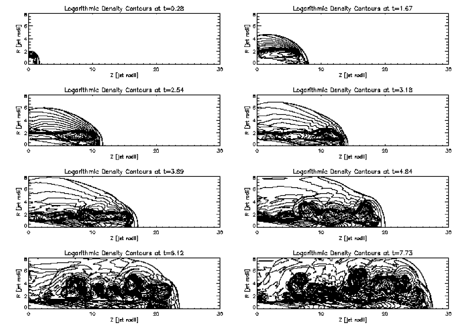
Figure 1: Contour plots of the density (30 logarithmically spaced lines) for the jet model of setup A. The times for the snapshots were chosen in order to match Fig. 11 of KM (88) closely.

2 Description of the codes

The reference codes are a two dimensional MHD code by Lind (Lind (1986); LPMB (89)), named FLOW, and an also two dimensional HD code by Kössl (KM (88)), hereafter DKC. A precise description of FLOW can be found only in Lind’s Ph.D. thesis (Lind (1986)). There, Lind points out two special features of FLOW. First, it uses a predictor corrector algorithm for the timestep calculation and second, a specific advection method is applied. This method considers the matter density flux as the primary advective quantity and calculates the remaining fluxes by multiplying the matter density by the specific density in the cell origin. It is not a Godunov scheme, and does not use an exact or approximate Riemann solver. The code that we used for the recomputations was NIRVANA (Ziegler & Yorke (1997)), capable of three dimensional computations but used here in the 2D mode. The latter has like the others accomplished the usual tests and has already been used in simulations of proto-stellar jets (Thiele (2000)) and other astrophysical problems (e.g. Ziegler & Ulmschneider (1997)). All these codes use explicit Eulerian time stepping. They are second order accurate and use a monotonic upwind differencing scheme. They treat the following standard set of ideal (magneto-) hydrodynamic equations:

$$\frac{\partial\rho}{\partial t}+\nabla\cdot\left(\rho{\bf v}\right) = 0$$ (1)

$$\frac{\partial\rho{\bf v}}{\partial t}+\nabla\cdot\left(\rho{\bf v}{\bf v}\right) = -\nabla p+\frac{1}{4\pi}\left({\bf B}\cdot\nabla\right){\bf B}-\frac{1}{8\pi}\nabla{\bf B}^{2}$$ (2)

$$\frac{\partial e}{\partial t}+\nabla\cdot\left(e{\bf v}\right) = -p\;\nabla\cdot{\bf v}$$ (3)

$$\frac{\partial{\bf B}}{\partial t} = \nabla\times({\bf v}\times{\bf B}),$$ (4)

where $\rho$ denotes the density, $e$ internal energy density, ${\bf v}$ velocity, ${\bf B}$ the magnetic field and $p=(\gamma-1)e$ the pressure. Here $\gamma=5/3$ for a nonrelativistic monoatomic gas is assumed. Instead of the internal energy $e$, FLOW and DKC use the total energy $u=\rho v^{2}/2+e+B^{2}/8\pi$. Equation (3) is then replaced by:

$$\frac{\partial u}{\partial t}+\nabla\cdot\left(u{\bf v}\right)=-\nabla\cdot(p{\bf v}).$$ (5)

This is analytically equivalent, but may give different numerical results, in particular in regions of discontinuous flows. Another difference of the codes is the use of artificial viscosity. FLOW has no need for artificial viscosity at all, according to test calculations reported in Lind (1986). DKC and NIRVANA use an artificial viscosity in order to enhance the diffusion in regions of strong gradients. This has the effect that shocks are transported correctly without numerical oscillations at the cost of smoothing the shocks over some grid zones. DKC even makes use of an antidiffusion term, which cancels the effects of artificial viscosity in regions of smooth flow. This point reflects the differences in the details of the implementation of the three codes as summarized in Table 1. Table 1. Differences between the discussed codes FLOW DKC NIRVANA uses e x uses u x x art. viscosity x x antidiffusion x

3 Hydrodynamic jet simulations

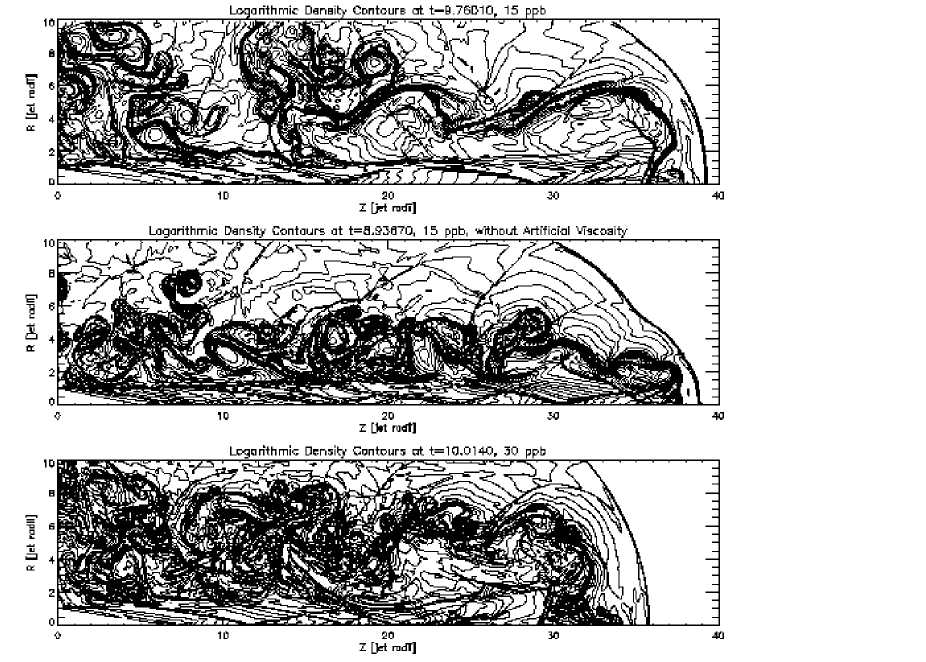
Figure 2: Logarithmic density plot of the jet from setup C. Top: 15 ppb resolution, t=9.76; middle: 15 ppb resolution without artificial viscosity, t=8.94; bottom: 30 ppb resolution, t=10.00

3.1 Numerical Setup

As is appropriate for the simulation of axially symmetric jets we use (normalized) cylindrical coordinates (r,z). The jet is injected into a homogeneous ambient medium. We take the density and the pressure there as the unit values. Therefore the sound speed in this external medium is $\sqrt{\gamma}$. The jets are injected in pressure equilibrium and have a density contrast of $\eta=0.1$ which means that the jet material has 0.1 times the density of the ambient medium. The unit of length is the jet radius $R_{\mathrm{j}}$. Velocity is measured in units of $\sqrt{p_{\mathrm{m}}/\rho_{\mathrm{m}}}$, where $p_{\mathrm{m}}$ is the pressure and $\rho_{\mathrm{m}}$ the density in the ambient medium, and the time unit is $R_{\mathrm{j}}/\sqrt{p_{\mathrm{m}}/\rho_{\mathrm{m}}}$. The units were chosen to match the normalized units in LPMB (89) and KM (88) as closely as possible. The boundary conditions are rotational symmetry at the jet axis, an outflow condition at the upwind boundary for setup A and an impenetrable wall for setup B and C (except for the nozzle). Open boundaries were applied on the two other sides besides setup C where outflow was specified in order to match the original conditions. This should have no noticeable effect, since inflows from those sides are hardly expected. The simulations are carried out at different resolution characterized by the number of grid points the jet beam is resolved with (ppb). We also add higher resolution images than the original computations. Setup A and B recompute the results from KM (88), where two simulations with higher resolution were added to setup B, and setup C is designed according to the hydrodynamic jet from LPMB (89). The parameters are summarized in Table 2. We note the following on the jet nozzle: In our MHD simulations we encountered problems when the boundary condition was applied in the usual one grid zone only. Therefore we fixed the jet values in an area of four cells from the upwind boundary. In the simulations without magnetic field, we did this in the same way, although it did not influence our results here. Table 2. Parameters of the jet models Setup A B C Jet velocity $v_{\mathrm{j}}$ 24.5 24.5 25.0 Resolution (ppb) 40 10,20,40,70, 15,30 100,200,400 upwind boundary outflow reflecting reflecting comp. area (in $R_{\mathrm{j}}$) 8$\times$30 4$\times$10 10$\times$40 reference code DKC DKC FLOW

3.2 Setup A: inter-code comparison of a time series

The time evolution of the jet model of setup A is shown in Fig. 1. Snapshot times were chosen very similar to the corresponding model in KM (88). Comparing the two computations, at the first glance, one recognizes a great similarity: In both cases at early times, a laminar backflow is established, where the terminal Mach disk is nearly perpendicular to the z-axis. At $t=3.18$ the laminar backflow phase terminates with the Mach disk becoming oblique and one of the forward and backward moving shocks from the beam extending into the backflow where it decelerates the backflow deflecting it away from the axis. The material to the left of this shock structure at approximately $z=8$ at $t=3.89$ is pumped off the grid and has disappeared at $t=6.13$. The rest of the backflow material essentially stays at its place until the end of the simulation expanding from 2 up to 6 jet radii. Also visible in our simulation are the crossing oblique shock waves in the beam. So far the described features matched the corresponding ones in the original publication very well. In Fig. 5 the bow shock velocity from our computation is compared to the one in the original publication. It shows a variation on the level of every evaluated timestep with an amplitude of roughly one in the Mach number. This was unrevealed in the original paper due to the lower sampling rate (23 versus 76 snapshots in our computation). The oscillation is modulated by a mode with longer wavelength (represented by the smoothed curve in Fig. 5) which is about 2 in our results and 1.7 in KM (88). They called this periodic de- and reaccelleration “beam pumping”. It was interpreted by Massaglia et al. (1996) in the following manner: The oblique shocks have a high pressure on the axis. Each time they arrive at the jet head, the head is accelerated due to this pressure gradient. Because of this phenomenon multiple bow shocks appear which can be seen in Fig. 1 (especially at $t=6.13$). The overall jet velocity decreases in the laminar phase in a similar way as in the DKC computation. But after $t\approx 4$ the decrease in our computation is faster. At $t=7.73$ our jet has approached $z=27.43$ which is $9\%$ less than the reference value. At a first glance it is surprising that the jet velocity decreases at all, for it can be derived very easily by equating the ram pressure of the jet, $\rho_{\mathrm{j}}(v_{\mathrm{j}}-v_{\mathrm{bow}})^{2}$ to the pressure in the external medium $\rho_{\mathrm{m}}v_{\mathrm{bow}}^{2}$ that the bow shock velocity should be constant:

$$v_{\mathrm{bow}}\approx\frac{\sqrt{\eta}\,v_{\mathrm{j}}}{1+\sqrt{\eta}},$$

where $\eta=\rho_{\mathrm{j}}/\rho_{\mathrm{m}}$ is the density contrast. For the jet under consideration this bow shock velocity should evaluate to $5.9$, approximately achieved in very early times of our simulation. The explanation for this decrease in the bow shock velocity was given by LPMB (89): As the jet propagates, its head expands and $\eta$ in the above formula has to be replaced by $\eta\epsilon$ with $\epsilon=A_{\mathrm{j}}/A_{\mathrm{head}}$ the ratio between the area of jet beam and its head. Taking this into account we conclude that the effective working surface for the jet is $\approx 3R_{\mathrm{j}}$ at late times of our simulation. This corresponds well to the extent of the jet head in our contour plots (Fig. 1). A clear discrepancy between the simulations is the appearance of the KH instabilities. Where in the original publication only an unstructured bump is visible, in our computation a round filigree system with additional instabilities can be seen. At this point we propose that the observed differences are caused by a different effective resolution of the two codes (This question will be examined in more detail in Sect. 3.4). So one can say that the qualitative behavior of the simulation is well reproduced, which gives additional confidence in the quality of both simulations. But on a quantitative level there are differences. The NIRVANA jet is slower at late times and develops a richer cocoon structure. The differences arise in the non-laminar flow phase.

3.3 Setup C: the effect of artificial viscosity

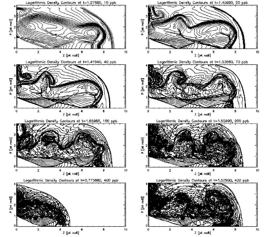
Figure 3: Jets from setup B. 30 logarithmically spaced density contours are shown. Time and resolution are indicated on top of the individual pictures.

The reference paper for this subsection is LPMB (89). They plot their hydrodynamic jet model at t=10 (in our units). This is not possible for our recomputation because at t=10 the NIRVANA jet has left the computational domain. For that reason, we discuss the last timestep with the bow shock not having left the grid ($t=9.76$, see Fig. 2). At a first glance, it seems that our jet differs quite a lot from the reference jet: It propagates faster (average velocity of 4 versus 3.5), the region between bow shock and contact discontinuity on the axis (at z $\approx$ 36 in Fig. 2) extends over one jet radius (versus three, compare Fig. 6), the inner beam shock structure is by far more irregular in our computation and this prevents the cocoon from developing regular vortices. In the original publication the cocoon extended everywhere over about 7 jet radii, whereas at the end of our simulation one vortex has even started to leave the grid over the upper boundary. Why are there such strong differences? In order to investigate this question we performed the simulation again with twice the resolution (Fig. 2). The result is striking. The average velocity reduces to 3.6 which is only 2% higher than the 3.5 reference value. The region between bow shock and contact discontinuity is amplified to two jet radii (compare Fig. 7), the cocoon extends over 8 jet radii, approximately, and in the interior of the beam there are more oblique shocks. This strongly suggests that with a little bit more than twice the resolution NIRVANA reproduces the global parameters achieved in the FLOW simulation. Another reason for the differences might be the shock handling by methods of artificial viscosity in NIRVANA. Therefore, we have repeated the simulation at the original resolution (15 ppb), but without artificial viscosity. We note here that artificial viscosity is not an option but a necessity in order to handle shocks correctly for NIRVANA. Fig. 2 shows that there is now almost nothing of the cocoon material accumulating on the left hand boundary. Instead most of it is consumed in KH instabilities of approximately equal wavelength than in the original publication. There are more oblique shocks in the beam, too. We conclude, that Lind’s hydrodynamic jet simulation is, strictly speaking, not reproducible by our code. But we can explain the shape of the cocoon by the different diffusivity description in Lind’s code and the global parameters by a doubling of the resolution in NIRVANA. The comparison between our 15 ppb model and our 30 ppb model clearly shows a strong dependence of the growth of the KH instability on the resolution.

3.4 Setup B: the numerical convergence of a hydrodynamic jet in comparison to KM (88)

3.4.1 Details of the flow

The results are shown in a series of logarithmic density plots in Fig. 3. The times for the snapshots were chosen in order to match the one in the original computation with an accuracy of better than one percent. Comparing the contour plots with the results from KM (88) one can immediately see that they are very similar with the exception that we needed only about half the resolution to achieve the same result: At the resolution of 10 ppb we get the conspicuous ledge at $(r,z)\approx(1.5,8)$ of the contact discontinuity which appears only at 20 ppb in the original. The hook like structure at $(r,z)\approx(3,1)$ can be seen for the first time in the 20 ppb plot at ours and looks almost identical to the 40 ppb picture in KM (88). With NIRVANA we are able to resolve internal shock waves with our lowest resolution (10 ppb versus 20 ppb). Crossing shock waves become visible at 20 ppb (versus 40 ppb) and the upper right one of the cross like shocks appears at 40 ppb (versus $\approx$ 70 ppb). The inner beam also consists of plane and centered rarefaction waves (see KM (88) for details) which one can identify at 10 ppb in our simulation (versus 20 ppb). The cocoon is dominated by a prominent KH instability of wavelength $\approx 4$ in the original publication which becomes somewhat shorter in our simulations. It appears as a break in the contact discontinuity at low resolution. At 70 ppb in our simulation a round structure has formed which, approximately, retains this size up to 200 ppb. Only a part of the interior of this structure develops higher mode KH instabilities. This means that this region becomes turbulent. No sign of that can be seen in the DKC simulations. They resolve KH instabilities on the level of breakpoints in the contact discontinuity even at 100 ppb.

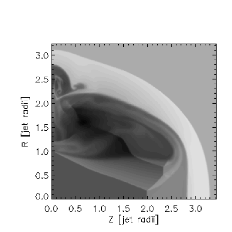
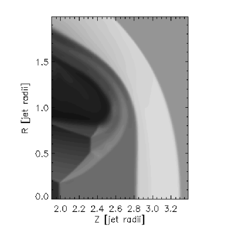
a b

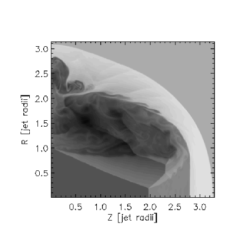
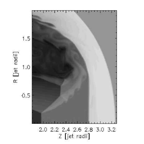
c d

Figure 4: Gray scale plots of the logarithmic density for the jets of setup B. On the right hand side are magnifications of the head region of the corresponding picture to the left. The upper (a and b) and lower (c and d) pictures show the 100 ppb and 200 ppb simulations, respectively. The time is 0.500 in all cases.

Figure 5: Bow shock velocity over time for the jet of setup A (solid line), smoothed (long dashed line) and for comparison the approximate behavior in KM88 adopted from their figure 9a (short dashed line). 76 time steps were used for this graph.

Figure 6: Flow parameters for the hydrodynamic jet model of setup C at 15 ppb with shock handling by artificial viscosity. The vertical axis displays the z-coordinate and the horizontal axis the time in our units which is 1/15 of Lind’s time unit. The highest z-value has always the bow shock, the contact discontinuity has a lower or equal z-value and the Mach disk takes the lowest value.

Figure 7: Same as Fig. 6, but at a higher resolution of 30 ppb.

3.4.2 Kelvin-Helmholtz instabilities at the contact discontinuity and beam boundary

At our highest resolution of 400 ppb we discover for the first time a completely different behavior of the KH instability. A close look at Fig. 3 shows that the amplitude of the dominant KH mode in the cocoon, which is continously growing at lower resolution, is only about half as big in the 400 ppb plot as in the 200 ppb plot. Furthermore, the contact discontinuity is turbulent almost everywhere, already at earlier times, when the dominant mode was not yet evolved (see lower left picture in Fig. 3). This is quite contrary to the situation at lower resolution, where the longest wavelength mode develops first. A gray scale plot of the logarithmic density for the three highest resolution simulations at time $t\approx 0.5$ is shown in Figs. 4 and 8. It shows that at 100 ppb the contact discontinuity between shocked ambient medium and jet backflow is smooth. This changes at 200 ppb. Here at about $R=2$, evolved KH instabilities show up over about one jet radius. In the magnification, one can see that a high density flow emerging from the triple shock point at the Mach disk, which is also present at lower resolution, develops also KH instabilities. These two seem to interact with each other. In the 400 ppb gray scale plots, the bumps of the first one are located in immediate vicinity of the bumps of the other one. In the 200 ppb plot at $R\approx 0.8$, the bump in the inner flow even seems to hit the contact discontinuity. Furthermore, the two phenomena arise at the same resolution threshold. The bumps in the contact discontinuity are not stationary. They move to the left (see Fig. 9d).

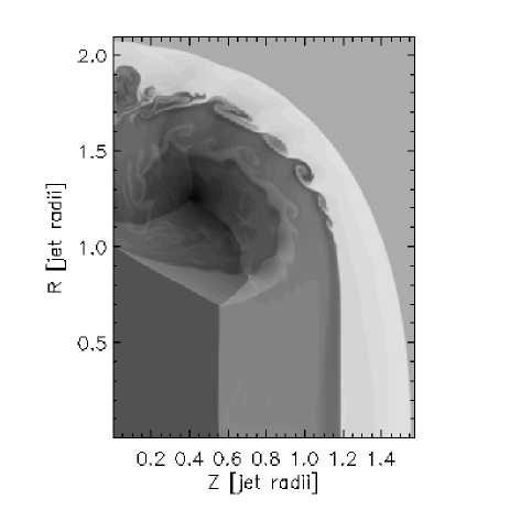
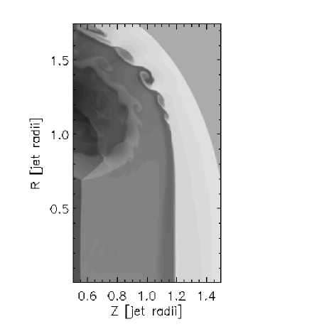
a b

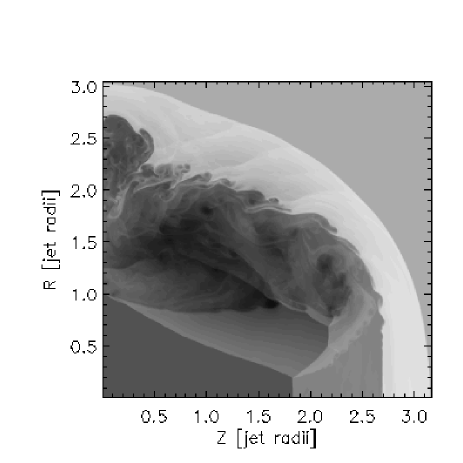
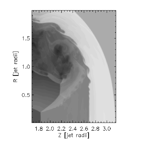
c d

Figure 8: Same as 4 but for 400 ppb and at times t=0.216 (upper pictures) and t=0.483 (lower pictures). (The data in this figure and in Fig. 4 was rebinned to 100 ppb for visualization.)

The backflow of the jet gas in the vicinity of the contact discontinuity has a velocity of about 12 towards the left. It accelerates the almost only outward moving shocked external medium to velocities in excess of 7, which is about $30\%$ of the jet velocity. Because of that motion, the KH instabilities in the head region of the jet are always small in this early phase. These moving KH instabilities act like a piston on the shocked external medium. They drive weak waves, 3 of which are seen in the lower left plot of Fig. 3. Indeed, their appearance can be best seen in the radial slices of the density and radial velocity (Fig. 9a-c). The resolution comparison shows at 100 ppb in the region between $R\approx 2$ and $R\approx 2.7$ a nearly linear density increase. At 200 and 400 ppb the peaks of the discussed waves are clearly visible. Thus, it seems that the stream from the Mach disk triple shock point causes the KH instabilities at the contact discontinuity, which in turn drives weak waves into the shocked external medium.

a b

c d

Figure 9: a-c: Slices at $Z=1.5$ for radial velocity (solid) and density ($-6$) (dashed) over grid points at time t=0.5 for setup B. The resolution is 100, 200, and 400 ppb for plot a to c, respectively. The shocked external medium is located between $R=2$ and $R=2.7$. d: Radial slice for density ($\cdot 10$) and axial velocity at t=0.5, Z=1.5 for the 400 ppb simulation. At R=1.9 the fingers of the KH instabilities are visible (increase in the density). They also appear in the velocity as slower regions.

Small KH instabilities are also observed at the beam boundary, at highest resolution (Fig. 3). They move towards the jet head. For example, the biggest bump in the lower plots of Fig. 3 is located at $Z\approx 2$ in the left hand plot and at $Z\approx 3$ in the right hand plot. It depends on their velocity if they can be dangerous for the beam stability before they reach the jet head.

3.4.3 Rayleigh-Taylor instabilities at the jet head

Furthermore, the “beam pumping” (see above) gives rise to the onset of Rayleigh-Taylor (RT) instabilities near the axis in the contact discontinuity, which appear for the first time at a resolution of 100 ppb in the original publication, but can be clearly identified in our 70 ppb contour plot ($(r,z)\approx(0.5,7.5)$). Close examination of the jet head (Fig. 3 ,4, and 8) reveals that also the development of RT instabilities is crucially dependent on the resolution. The RT instability needs an accelerating jet, which only appears at a certain resolution threshold connected to the appearance of oblique shocks in the jet, which are responsible for the acceleration. In order to investigate the mass entrainment into the jet head in more detail, we show the radial average of the density in the jet beam (Fig. 16). In the low resolution plots, the contact discontinuity is visible as a nearly vertical line joining the density in the beam at nearly 90 degree. At 70 ppb small peaks appear at the contact discontinuity. This is the first sign from the RT instability. At higher resolution the differences between five and eight jet radii become more pronounced. At 400 ppb, the density in the region between $R=5$ and $R=7.5$ exceeds the density in the 10 ppb simulation by 0.2, on average. This corresponds to an entrained mass of about $\rho_{\mathrm{m}}R_{\mathrm{j}}^{3}$.

3.4.4 Convergence of global quantities

We have also computed some global quantities for each simulation. Fig. 12 shows that at every resolution our jet is slower than its counterpart in the original publication by $\approx(4.5\pm 2)\%$. If we use in NIRVANA a lower resolution by a factor of $2-2.5$ than the corresponding computation in the original publication we get the same average bow shock velocity. Fig. 13 shows the convergence of four global quantities up to the highest resolution. The first two are the bow shock velocity averaged over the computation time and the total mass in the computational domain. These two parameters should be coupled because the bow shock sweeps the mass, which is concentrated in the ambient medium, off the grid. They converge at 100 ppb. This reflects the fact that the cocoon develops only additional small scale structure once the long wavelength instability has been sufficiently resolved. The behavior changes at 400 ppb, where again more matter remains within the computational domain after a stagnation between 100 and 200 ppb. Axial momentum is mainly situated in the region between contact discontinuity and bow shock (shroud), the beam and the backflow (decreasing order). In all the simulations compared in Fig. 13, the axial momentum changes by only 5% indicating that the global flow pattern is reproduced quite well already at low resolution. The internal energy is concentrated in the region behind the bow shock and in front of the Mach disk. This is why it is partly correlated to the axial momentum. But convergence of this number indicates also a correct description of the terminal shock region. As can be seen in Fig. 3, the terminal shock region seems to behave quite differently in simulations with different resolution. Changes of the internal energy on the 5% level remain up to 200 ppb. The flat behavior between 200 and 400 ppb might be due to coincidence.

Summarizing, it seems that the simulation was well on its way to convergence up to 200 ppb. But the surprising damping of the long wavelength KH instability opened up a new chapter in the convergence behavior.

4 Magnetohydrodynamic jet simulations

4.1 Configuration

The setup here is essentially the same as in setup C of the previous section except for a toroidal magnetic field ($B_{\phi}$) and a jet pressure profile which assures initial transverse hydromagnetic equilibrium (see LPMB (89) for details). The jet profile is:

$$B_{\phi}=\left\{\begin{array}[]{r@{\quad,\quad}l}B_{\mathrm{m}}\;r/R_{\mathrm{m}}&0\leq r<R_{\mathrm{m}}\\ B_{\mathrm{m}}\;R_{\mathrm{m}}/r&R_{\mathrm{m}}\leq r<R_{\mathrm{j}}\\ 0&R_{\mathrm{j}}\leq r\end{array}\right.$$ (6)

and

$$p=\left\{\begin{array}[]{r@{\quad,\quad}l}\left[\alpha+\frac{2}{\beta_{\mathrm{m}}}\left(1-\frac{r^{2}}{R_{\mathrm{m}}^{2}}\right)\right]p_{\mathrm{m}}&0\leq r<R_{m}\\ \alpha\;p_{\mathrm{m}}&R_{\mathrm{m}}\leq r<R_{\mathrm{j}}\\ p_{\mathrm{m}}&R_{\mathrm{j}}\leq r\end{array}\right.$$ (7)

where $R_{\mathrm{m}}=0.37(R_{\mathrm{j}})$, $B_{\mathrm{m}}=11.09$, $\alpha=0.33$, and $\beta_{\mathrm{m}}=0.205$. The average plasma $\bar{\beta}$ which gives the ratio of the mean internal gas pressure to mean internal magnetic pressure is defined as:

$$\bar{\beta}:=\frac{\bar{p}}{\frac{1}{8\pi}\frac{2}{R_{\mathrm{j}}^{2}}\int_{0}^{R_{\mathrm{j}}}B^{2}_{\phi}(r^{\prime})\;r^{\prime}\;dr^{\prime}}$$ (8)

and has the value of 0.6. The mean magneto-sonic Mach number,

$$\bar{M}_{\mathrm{j}}=v_{\mathrm{j}}(\frac{2}{R^{2}_{\mathrm{j}}}\int_{0}^{R_{\mathrm{j}}}(\gamma+B_{\mathrm{\phi}}^{2}/(4\pi p))\frac{p}{\rho}\;r\prime\;dr\prime)^{-1/2},$$ (9)

is 3.5. This corresponds to the highly magnetized jet model in LPMB (89).

4.2 Comparison of results

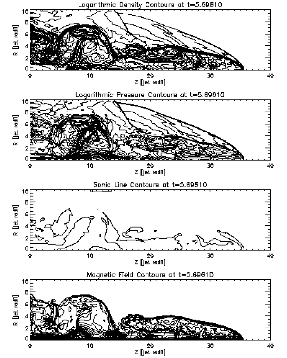
Figure 10: Contour plots of the density (30 logarithmically spaced lines), pressure (30 logarithmically spaced lines), magneto-sonic lines (magneto-sonic Mach number equals 1 or -1) and toroidal magnetic field (30 lines) of the highly magnetized jet model at timestep 13500. This corresponds to a simulation time of 5.70. In units of LPMB (89) that would be 85.5.

Detailed contour plots of the MHD jet at the end of the simulation are given in Fig. 10. At first sight, one recognizes a great similarity to the corresponding picture in LPMB (89). The same nearly stationary big terminal vortex forms which includes the Mach disk. Here the jet material is driven away from the axis out to about $r=6$, where it is partly refocused onto the axis due to the Lorentz force, and another part manages to establish a backflow. This backflow turns again joining the main stream. As can be seen quite well in the sonic line plot the refocused material hits the z-axis at about $z=13$. There it separates itself again, forming an on-axis backflow (which enhances the deflection from the axis and then joins the main stream) and a time dependent outflow from the region in the z-direction which leaves at $z\approx 15$. Due to the low pressure and the high magnetic field ($\beta\equiv 8\pi p/{\bf B}^{2}\approx 10^{-2}$), this area was called magnetically dominated cavity by LPMB (89). This is reproduced well in our simulation. When the plasma leaves this cavity, it forms a so called nose-cone of about $4\,R_{\mathrm{j}}$ width, as it should be. This nose-cone ends at a contact discontinuity which can be seen in the plot of the toroidal magnetic field. At $t=5.7$ (Fig. 10) the bow shock has an average velocity of 6.27 which is about 3% slower than the corresponding jet in LPMB (89). This might be due to the accuracy of the measurement which was carried out using an ordinary ruler for z-position of the bow shock in Lind’s publication and dividing it by the simulation time. The advance of bow shock, Mach disk and contact discontinuity is shown in Fig. 14 and is generally very similar to the corresponding picture in LPMB (89). The exception is the position of the Mach disk, which has a considerably lower z-value in our simulation. At $t\approx 5.7$ our Mach disk has reached $z\approx 5$ versus $z\approx 7$ in the original publication. The advance of the Mach disk seems to be coupled to the size of the on-axis backflow described above.

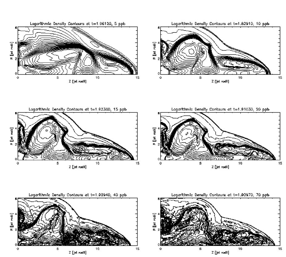
Figure 11: Snapshots of the logarithmic density contours of the MHD jet at different resolutions. Times of the snapshots and resolution are indicated on top of the individual figures.

Figure 12: Comparison of the bow shock velocity of the setup B jets with the ones of equal snapshot time from KM (88). The snapshot times were: 10 ppb: t=1.28, 20 ppb: t=1.41, 40 ppb: t=1.42, 70 ppb: t=1.99 and 100 ppb: t=1.98.

Figure 13: The total values of internal energy, axial momentum, mass and average bow shock velocity against resolution for the simulations from setup B. At the resolution of 100 the mass is converged with an accuracy of 3 digits. Here t=1.28 except for 70 ppb were t=1.27.

Figure 14: Time evolution of bow shock, Mach disk and contact discontinuity for the simulation of Fig. 10. Notice that there is only a small difference between the positions of contact discontinuity and bow shock.

Figure 15: On axis ($r=1/15$) gas and magnetic pressure for the simulation of Fig. 10. The upper line displays the gas pressure and the lower one the magnetic pressure. Note the close relationship between them.

The amount of this on-axis backflow turns out to be sensible to the code used for the simulation: It is stronger in our simulation and therefore the Mach disk moves slower. We have plotted gas and magnetic pressure close to the axis in Fig. 15. One can see the close correlation of the magnetic pressure and the gas pressure. Directly on the axis the magnetic field vanishes because of axi-symmetry. Therefore the magnetic field is generally weak in vicinity to the jet axis. The plot confirms also the original publication: Behind the Mach disk the gas pressure rises up to 60 and in the nose-cone it is on average $25-30$. In all our magnetized jet simulations, we do not find any RT instability. In contrast, we do find one prominent KH instability developing at the upper right edge of the big vortex, probably excited by the jet stream that hits the contact discontinuity here. This was not observed in the original publication. The instability circled around the vortex and deposited an amount of jet plasma to the left of the vortex where one can see shocked ambient gas in the original publication. Other differences are the shock structures in the nose-cone. They are sharper in the original which one can trace back to the lower amount of diffusivity in shock regions by the FLOW code (compare also setup C of our hydrodynamic section).

4.3 Convergence

To investigate the convergence behavior we repeated the simulation at lower and at higher resolutions (5 ppb, 10 ppb, 20 ppb, 40 ppb and 70 ppb). The results are shown in Fig. 11. The time chosen for the snapshots was approximately 1.9. At that time the KH instability is excited as a bump at $(r,z)\approx(3.5,6)$. Interestingly, this bump disappears at a resolution of 70 ppb like in the original publication. The behavior of the internal structure of the nose-cone does not seem to converge. The Mach disk moves slower at higher resolution. It has advanced $\approx 0.2\,R_{\mathrm{j}}$ less at 20 ppb than at 15 ppb in Fig. 11. At 70 ppb the Mach disk has reached the inflow boundary. Already at 40 ppb the shape of the contact discontinuity changes. This is probably due to the vicinity of the Mach disc to the inflow boundary. The retreat of the Mach disk is surprising. Given higher efficiency of FLOW, we should compare the 20 or 40 ppb simulation to the FLOW result. Therefore the two simulations seriously disagree on the propagation of the Mach disk, and it seems that NIRVANA approaches convergence in a different way than FLOW, at least, if a dominant magnetic field is present. Nevertheless the overall shape of the bow shock and the contact surface remains essentially the same. Also the average bow shock velocity stays remarkably constant, 7.6 at 15 ppb and 7.5 at the others: It seems to be converged. With an eye on the lower resolution plots we could say that even 10 ppb are sufficient to catch the correct behavior at the contact discontinuity and the bow shock. But there is a sharp transition to lower resolution. This tells us that the essential features dictating the shape of the bow shock and essentially also of the contact discontinuity are of the order $1/10$ of a jet radius.

5 Discussion

We have carried out simulations of magnetized and unmagnetized astrophysical jets in 2D. In the pure hydrodynamic simulations, we showed by detailed examination of a time series which was compared to the simulation by Koessl & Müller (1988) and by a recomputation of the model of LPMB (89) that in principle each of the evaluated codes is able to produce similar results. However they do not achieve this result with the same resolution: DKC needs more than twice the resolution to achieve similar results compared to NIRVANA. NIRVANA in turn needs somewhat more than twice the resolution in order to achieve the same results as FLOW. Our results have revealed that depending on the exact method of shock handling the effective resolution of MHD codes – measured through the convergence of global variables and inspection of characteristic features in the contour plots by eye – differs considerably more than in the test calculations by Woodward and Colella (1984) – when applied to the jet propagation problem. If one looks at results produced by the codes at moderate resolution (20 - 40 ppb) we find a characteristic representation of KH instabilities: they appear as breaks in the contact discontinuity in DKC, as round structures in FLOW and as intermediate a little bit unregular but still round structures in NIRVANA. While FLOW is quite an unusual code, because it needs no artificial viscosity, it turns out to be the most efficient code by far, at least, if no magnetic field is present. Strictly speaking, we cannot reproduce the results of FLOW with NIRVANA. But the differences are explained by effects of resolution and artificial viscosity together. We also have shown that the resolution of the simulation influences the average bow shock velocity more in the non-laminar flow phase than in the laminar one. Because we explain the differences between the codes with a resolution effect, we conclude that in the laminar phase the beam structure is indeed converged whereas in the non-laminar one it is not. We find that the global jet parameters are converged in HD simulations with NIRVANA at $\approx$ 100 ppb. But even with our highest resolution computation (400 ppb) we do not achieve a fully converged beam structure: There are KH instable regions in the cocoon and a complicated terminal shock structure that seems to evolve in a turbulent manner. On the contrary, on the highest level of resolution qualitatively new behavior arises: the long wavelength KH instabilities are damped by the onset of small-scale turbulence, which develops prior to the long wavelength modes, and the RT instability manages to entrain more and more mass into the jet’s head with increasing resolution. In a real situation however, one can expect that KH instabilities at the contact discontinuity will arise because of inhomogeneities in the external medium or a not completely steady jet flow. The present computation shows that they arise, even with a homogeneous external medium and a steady jet flow.

Concerning the jet with a toroidal magnetic field we found a good convergence behavior up to 20 ppb: Already at 10 ppb the shape of the bow shock and the contact discontinuity is essentially converged. The average bow shock velocity changes only slightly up to 20 ppb. (It remains constant for higher resolution.) A big problem is the discovered moving of the Mach disk towards the inflow boundary. It tells us that this particular simulation does not converge, when computed with NIRVANA. It would be interesting to check this result for different initial conditions. A better configuration for the jet with a toroidal magnetic field would probably be one with a time dependent injection like the outflow from the magnetically dominated cavity. Furthermore this is a serious disagreement between FLOW and NIRVANA. One possible explanation could be that the efficiency derived in the hydrodynamic case can not be applied for simulations with a magnetic field, maybe, because the different diffusivity description puts NIRVANA and FLOW on two different convergence branches. How the propagation of the Mach disk would change with resolution for the FLOW case remains unclear. Resolution studies with different codes are therefore desirable.

a b

c d

e f

Figure 16: Density averaged over the beam radius for the simulations of setup B. Plots a to f apply to 20 ppb, 40 ppb, 70 ppb, 100 ppb, 200 ppb and 400 ppb, respectively. The mass entrainment into the jet head can be seen in plot f, between $Z=6$ and $Z=7.5$. For comparison, the 10 ppb curve is plotted as a dashed line in each figure.

References

- Aloy et al. (1999) Aloy, M.A., Ibanez, J.Ma., Marti, J.Ma., Gomez, J.L. and Müller, E. 1999, ApJ, 523, L125-L128
- Appl & Camenzind (1992) Appl, S., Camenzind, M. 1992, A&A, 256, 354-370
- Appl (1996) Appl, S. 1996, A&A, 314, 995-1002
- Blandford & Rees (1974) Blandford, R.D., Rees, M.J. 1974, MNRAS, 169, 395
- Bodo et al. (1994) Bodo, G., Massaglia, S., Ferrari, A., Trussoni, E. 1994, A&A, 283, 655
- Bodo et al. (1995) Bodo, G., Massaglia, S., Rossi, P., Rosner, R., Malagoli, A., Ferrari, A. 1995, A&A, 303, 281
- Bodo et al. (1998) Bodo, G., Rossi, P., Massaglia, S., Ferrari, A., Malagoli, A., Rosner, R. 1998, A&A, 333, 281
- Clarke et al. (1986) Clarke, D.A., Norman, M.L. and Burns, J.O. 1986, ApJ, 311 L63-L67
- Ferrari (1998) Ferrari, A. 1998, ARAA, 36, 539-598
- Hardee et al. (1997) Hardee, P.E., Clarke, D.A., Rosen, A. 1997, ApJ, 485, 533-551
- Komissarov (1999) Komissarov, S.S. 1999, MNRAS, 308, 1069-1076
- KM (88) Kössl, D., Müller, E. 1988, A&A, 206, 204-218
- Kössl et al. (1990) Kössl, D., Müller, E. and Hillebrandt, W. 1990, A&A, 229, 378-396
- Lind (1986) Lind, K.R. 1986, Ph.D. thesis, California Institute of Technology, USA
- LPMB (89) Lind, K.R., Payne, D.G., Meier, D.L. and Blandford, R.D. 1989, ApJ, 344, 89-103
- Massaglia et al. (1996) Massaglia, S., Bodo, G., Ferrari, A. 1996 A&A, 307, 997-1008
- Micono et al. (2000) Micono, M., Bodo, G., Massaglia, S., Rossi, P., Ferrari, A., Rosner, R. 2000, A&A, 360, 795-808
- Norman et al. (1982) Norman, M.L., Smarr, K.-H., Winkler, A. and Smith, M.D. 1982, A&A, 113, 285-302
- Rosen et al. (1999) Rosen, A., Hardee, P.E., Clarke,D.A., Johnson, A. 1999, ApJ, 510, 136-154
- Ryu et al. (1998) Ryu, D., Miniati, F., Jones, T.W. and Frank, A. 1998, ApJ, 509, 244-255
- Sod (1978) Sod, G. 1978, J. Comp. Phys., 27,1
- Thiele (2000) Thiele, M. 2000, Ph.D. thesis, University of Heidelberg, FRG
- Woodward & Colella (1984) Woodward, P., Colella, P. 1984, J. Comp. Phys., 54,115
- Ziegler & Ulmschneider (1997) Ziegler, U., Ulmschneider,P. 1997, A&A, 327, 854
- Ziegler & Yorke (1997) Ziegler, U., Yorke, H. 1997, Comp. Phys. Comm., 101, 54