The Glass-like Universe:
Real-space correlation properties of standard cosmological models

Abstract

After reviewing the basic relevant properties of stationary stochastic processes (SSP), defining basic terms and quantities, we discuss the properties of the so-called Harrison-Zeldovich like spectra. These correlations, usually characterized exclusively in $k$-space (i.e. in terms of power spectra $P(k)$), are a fundamental feature of all current standard cosmological models. Examining them in real space we note their characteristics to be a negative power law tail $\xi(r)\sim-r^{-4}$, and a sub-poissonian normalised variance in spheres $\sigma^{2}(R)\sim R^{-4}\ln R$. We note in particular that this latter behaviour is at the limit of the most rapid decay ($\sim R^{-4}$) of this quantity possible for any stochastic distribution (continuous or discrete). This very particular characteristic is usually obscured in cosmology by the use of Gaussian spheres. In a simple classification of all SSP into three categories, we highlight with the name “super-homogeneous” the properties of the class to which models like this, with $P(0)=0$, belong. In statistical physics language they are well described as glass-like. They do not have either “scale-invariant” features, in the sense of critical phenomena, nor fractal properties. We illustrate their properties with some simple examples, in particular that of a “shuffled” lattice.

]

I Introduction

In standard theories of structure formation in cosmology the density field in the early Universe is described as a perfectly homogeneous and isotropic matter distribution, with superimposed tiny fluctuations characterized by some particular correlation properties (e.g. [1]). These fluctuations are believed to be the initial seeds from which, through a complex dynamical evolution, galaxies and galaxy structures have emerged. In particular the initial fluctuations are taken to have Gaussian statistics and a spectrum which is exactly, or very close to, the so-called Harrison-Zeldovich (hereafter H-Z) [2, 3] or “scale-invariant” power spectrum (hereafter PS). Because fluctuations are Gaussian, the knowledge of the PS, or its Fourier conjugate, the real space correlation function, gives a complete statistical description of the fluctuations. The H-Z type spectrum was first given a special importance in cosmology with arguments for its “naturalness” as an initial condition for fluctuations in the framework of the expanding universe cosmology, and it is in this context that the use of the term “scale-invariant” to designate it can be understood. It subsequently gained in importance with the advent of inflationary models in the eighties, and the demonstration that such models quite generically predict a spectrum of fluctuations of this type. Since the early nineties, when the COBE experiment [4] measured for the first time fluctuations in the temperature in the Cosmic Microwave Background Radiation (hereafter CMBR) at large scales, and found results consistent with the predictions of models with a H-Z spectrum at such scales, the H-Z type spectra have become a central pillar of standard models of structure formation in the Universe. The aim of the present paper is twofold. Firstly, to clarify the statistical properties in real space of these distributions, which have been almost completely overlooked in the literature on the subject. And secondly, through this discussion, to relate and compare this model of the primordial Universe to correlated systems encountered in statistical physics. We attempt to make the paper as self-contained as possible, and not excessively technical in its discussion either of cosmology or statistical concepts, in the hope that it may be easily accessible to both cosmologists and statistical physicists.

The H-Z spectrum arises in cosmology through a particular condition applied to perturbations of Friedman-Robertson-Walker (FRW) models, which describe a homogeneous Universe in expansion. This condition - commonly referred to in cosmology as “scale invariance” of the perturbations - gives rise to a spectrum (commonly called the “scale-invariant” perturbation spectrum) with $P(k)\sim k$ at small $k$. All current standard cosmological models of structure formation in the Universe assume a spectrum exactly like this, or close to it, as initial condition for perturbations in the Universe. In such models there is at any time a finite scale corresponding to the causal horizon, which increases with time, and below which causal physics can act to modify the spectrum. This causal physics depends, in general, on the details of the model, i.e. on the nature of its content in matter and radiation (or other forms of energy), until a characteristic time (the time when matter and radiation have comparable densities), after which purely gravitational evolution takes over. There are many variants on standard cosmological models e.g. “Cold Dark Matter” (hereafter CDM), “Mixed Dark Matter” (hereafter MDM), or the currently favored one with a non zero cosmological constant (hereafter $\Lambda$CDM), each of them leading to a different form for the spectrum at smaller scales (i.e. large $k$) which can be calculated. In CDM models (in which the predominant massive component driving collapse under gravity is Cold Dark Matter, “cold” in the sense that the particles have little initial velocity dispersion) the PS decays at small scales (large $k$) as a negative power law in $k$, while in Hot Dark Matter (hereafter HDM) models (for which the prototype is a Universe dominated by a light neutrino) there is a exponential cut-off in the spectrum (due essentially to the fact that the “hot” neutrinos wipe out structures at these scales with their large velocity dispersion). All of these models, however, have the same “primordial” H-Z spectrum $P(k)\sim k$ (or very close to it) on large scales (i.e. small $k$), that is at scales which are large compared to the causal scale at the time of matter-radiation equality. This latter scale is of course much smaller than our present causal horizon (i.e. than the part of the Universe we can probe today). This means, in particular, that these primordial density correlations should be imprinted in the distribution of matter at very large scales, and should in principle be detectable in the distribution of galaxies at very large scales, inside the present horizon. Until now the only probe of fluctuations on such scales is through the temperature variations in angle of the CMBR, as the angular correlations in temperature fluctuations are coupled directly to the three dimensional density fluctuations. From the COBE measurements [4] the amplitude of the fluctuations inferred is $\sim 10^{-5}$ in the PS at these scales. We will discuss elsewhere the practical difficulties involved in measuring such a weak signal in the discrete distribution of galaxies. Here we concentrate on identifying the real space properties of these theoretical models at large scales.

Another context in which an understanding of the statistical properties in real space of the H-Z PS of the mass density field is important is represented by cosmological N-body simulations, the aim of which is to calculate the formation of structures under gravity in the Universe by a direct numerical calculation (see e.g. [5, 6]). Because the time scale of evolution in these simulations is short compared to the dynamical time of the system (i.e. a particle moves a small distance relative to the size of the box representing a large volume of the Universe) the final configuration depends strongly on the initial conditions (hereafter IC) at all but the smallest scales. Indeed a central idea is that from the final distribution - which should be closely related to the observed one of galaxies - one should be able to “reconstruct” some important features of the IC, which can be related to other observations such as those of the CMBR. A key issue for these simulations is thus the setting up of these IC, which involves subtle problems concerning the discretisation of the system. The usual approach to this problem is again entirely phrased in $k$-space, where instead a real space approach proves very useful [7]. To avoid any possible confusion for those somewhat familiar with these simulations, we note here at the outset that the description of the H-Z model we give in this paper, as lattice-like or glass-like, has no direct relation to the use of lattices or glasses in setting up IC in current N-body simulations. There lattices or glasses are understood to be sufficiently “homogeneous” configurations on which to superimpose fluctuations of a desired type. The reason for their use (instead of a “uniform” Poisson configuration) is purely numerical [7], and it has nothing to do with the intrinsic statistical properties of the systems being modeled. Indeed, as we will explain further at the appropriate below, these methods have been used primarily to simulate cosmological models at the smaller scales at which they are not at all glass-like.

Discussions of real space properties of the density fluctuations encountered in cosmology are puzzlingly sparse in the literature on the subject. Peebles briefly notes ([1] - see pg.523) that a very particular characteristic of H-Z models is that “on large scales the fluctuations have to be anti-correlated to suppress the root mean square mass contrast on the scale of the Hubble length”. Indeed, we emphasize the fact that these models are characterized at large scales by a correlation function $\xi(r)$ which has a negative power-law tail: detecting it would be the real space equivalent of finding the turnover to H-Z behavior to scales at which the PS goes as $P(k)\sim k$. The preference for a $k$-space description is probably rooted in the fact that the linear dynamics, which are used to describe many problems in cosmology, are most naturally treated in this space. While it is true of course that this description in $k$-space is complete, this by no means implies that the complementary real space view is redundant, as is well known in many contexts in physics. One of the points of this paper is to show that this complementary view of these apparently so familiar models is at the very least interesting and useful, in particular in how it facilitates comparisons with familiar physical systems.

A basic question we try to answer is the following: What “kind” of two-point correlation function is the one corresponding to the H-Z behaviour in cosmological models? We compare it to some different statistical homogeneous and isotropic systems: (i) Poisson-like distributions, (ii) systems with a power-law correlation function found in critical phenomena [10] and (iii) distributions characterized by long-range order (e.g. lattice or glass-like) [11]. Through this comparison we can classify H-Z models in the third category. We introduce the term “super-homogeneous” to refer to these kinds of distributions, as their primary characteristic is that mass fluctuations decay at large scales faster than in a completely uncorrelated (Poisson) system. For critical systems one has instead a decay of the mass variance which is slower than Poisson. Formally the definition of this class of “super-homogeneous” distributions is given by the condition that the PS has $P(0)=0$, or equivalently in real space that the integral of the two point correlation function over all space is zero. In the cosmological literature the latter property of cosmological models is often noted, but its meaning (as a strong non-local condition on a stochastic process) is not appreciated, or worse misunderstood as a trivial condition applying to any correlated system. In the textbook of Padmanabhan[12], for example, it is “proved” on pg. 171 that the integral over all space of the correlation function vanishes independently of the functional behaviour of $\xi(r)$. The error is in an implicit assumption made that the number of particles in a large volume in a single realization converges exactly to the ensemble average. This is not true because, in general, extensive quantities such as particle number have fluctuations which are increasing functions of the volume (e.g. Poissonian, for which the integral is not zero). A slightly different, but common, kind of misunderstanding of the meaning of the vanishing of the integral over the correlation function is evidenced in the book by Kolb & Turner [13]. There it is affirmed (after its statement in Eq.(9.39)) to be “…just a statement of mass conservation: if galaxies are clustered on small scales, then on large scale they must be “anti-clustered” to conserve the total amount of mass (number of galaxies)”. The source of this misconception seems to be a confusion with the so-called “integral constraint” in data analysis (e.g. [14, 15]), which imposes such a condition on the estimator of the correlation function in a finite sample, due to the fact that the (unknown) average number of points in such a sample is estimated by the (exactly known) number of points in the actual sample. Despite their apparent similarity, these are different conditions: the first (infinite volume) integral constraint provides non-trivial physical information about the intrinsic probabilistic nature of fluctuations, while the second is just an artifact of the boundary conditions which holds in a finite sample independently of the nature of the underlying correlations. We will discuss this point in a little more detail at the appropriate point below.

The paper is organized as it follows. In the first section we recall the basic properties of mass distributions (both continuous and discrete) described in terms of stationary stochastic processes with a well defined (non-zero) average density. In this context we introduce the basic statistical quantities (homogeneity scale, correlation functions, real space mass variance, PS etc.) used to describe these systems. We discuss in particular the relation between the mass variance in spheres and the PS, noting that for power law spectra $P(k)\sim k^{n}$ and $n\geq 1$, the small scale (i.e. large $k$) power dominates the real space variance at any scale. We explain that this is not a simple mathematical pathology but corresponds to a real property of these distributions. Indeed for discrete distributions of points we note that a theorem has been proved [16] showing the behaviour approached at $n=1$ to be the limiting decay of the variance, in real space spheres, in any distribution. In the subsequent section we discuss the H-Z spectrum, recalling the construction which leads to it in cosmology and why it is called “scale-invariant”. We note that the H-Z criterion, as naively understood, is not one which is satisfied exactly by the spectrum $P(k)\sim k$. In the next section we give a classification of all SSP in terms of the behaviour of the PS as $k\rightarrow 0$. We give the name “super-homogeneous” to those which have $P(0)=0$, referring to their basic characteristic as more homogeneous than the Poisson distribution, with a sub-poissonian decay of their mass variance. In the following section we give the examples of a lattice, and then a “shuffled” lattice, to illustrate the properties of distributions of this type, which have the strong order of a lattice or glass at large scales. Here we discuss also briefly the relation of our description to N-body simulations. In the final section we discuss various points in summarizing our findings. In particular we clarify the use of the term “scale-invariance”, “fractal” and “correlation length” in relation to the H-Z spectrum in cosmology.

II Basic Statistical Properties and Concepts

Inhomogeneities in cosmology are described using the general framework of stationary stochastic processes (hereafter SSP). Let us consider in general the description of a continuous or a discrete mass distribution $\rho(\vec{r})$ in terms of such a process. A stochastic process is completely characterized by its “probability density functional” ${\cal P}[\rho(\vec{r})]$ which gives the probability that the result of the stochastic process is the density field $\rho(\vec{r})$ (e.g. see Gaussian functional distributions [17]). For a discrete mass distribution the space (e.g. infinite three dimensional space) is divided into sufficiently small cells and the stochastic process consists in occupying or not any cell with a point-particle, and $\rho(\vec{r})$ can be written in general as:

$$\rho(\vec{r})=\sum_{i=1}^{\infty}\delta(\vec{r}-\vec{r}_{i})\,,$$ (1)

where $\vec{r}_{i}$ is the position vector of the particle $i$ of the distribution .

The stationarity refers in the present context to spatial stationarity of the process, and means that the functional ${\cal P}[\rho(\vec{r})]$ is invariant under spatial translation. This property is also called the statistical homogeneity of the distribution. We suppose also that the distribution is statistically isotropic (invariance of ${\cal P}[\rho(\vec{r})]$ under spatial rotation), and has a well defined average value $\rho_{0}$, that is

$$\langle\rho(\vec{r})\rangle=\rho_{0}>0\,,$$ (2)

where $\langle...\rangle$ is the ensemble average over all the possible realizations of the stochastic process, i.e. the average over the functional ${\cal P}[\rho(\vec{r})]$. Statistical homogeneity and isotropy (hereafter SHI) imply that the $l$-point correlation functions $\left<\rho(\vec{r}_{1})...\rho(\vec{r}_{l})\right>$, for any $l$, depend only on the scalar relative distances among the $l$ points [18]. Moreover we assume that ${\cal P}[\rho(\vec{r})]$ is ergodic. In order to clarify the meaning of ergodicity, let us take a generic observable $F=F(\rho(\vec{r}_{1}),\rho(\vec{r}_{2}),...)$ of the local density $\rho(\vec{r})$. Ergodicity means that $\left<F\right>$ is equal to the spatial average $\overline{F}$ given by:

$$\overline{F}=\frac{1}{\|\Omega\|}\int_{\Omega}d^{3}r_{0}F(\rho(\vec{r}_{1}-\vec{r}_{0}),\rho(\vec{r}_{2}-\vec{r}_{0}),...)$$ (3)

where the integral is extended to the whole space $\Omega$ and $\|\Omega\|$ is its (infinite) volume, and where $\rho(\vec{r})$ is (almost) any realization of the particle distribution “extracted” from the functional ${\cal P}[\rho(\vec{r})]$. This property is also referred as the self-averaging property of the distribution. Note that if the average in Eq. (3) is extended only to a finite sub-sample $V$ of the whole space $\Omega$ , then Eq. (3) is only an estimator of $\left<F\right>$ in the given sub-sample.

In a single realization of the mass distribution the existence of a well defined average density implies that [18]

$$\lim_{R\rightarrow\infty}\frac{1}{\|C(R;\vec{x}_{0})\|}\int_{C(R,\vec{x}_{0})}d^{3}r\,\rho(\vec{r})=\rho_{0}>0$$ (4)

where $\|C(R,\vec{x}_{0})\|\equiv 4\pi R^{3}/3$ is the volume of a sphere $C(R,\vec{x}_{0})$ of radius $R$, centered on the arbitrary point $\vec{x}_{0}$ of space . When Eq.4 is valid one can then define [18] a characteristic homogeneity scale as the scale $\lambda_{0}$ given by

$$\left|\frac{1}{C(R;\vec{x}_{0})}\int_{C(R;\vec{x}_{0})}d^{3}r\,\rho(\vec{r})-\rho_{0}\right|<\rho_{0}\;\;\forall R>\lambda_{0},\,\forall\vec{x}_{0}$$ (5)

which depends on the nature of the fluctuations of the density in spheres. In practice, in characterizing the scale at which a system begins to be homogeneous, it is easier to use directly some simple two-point statistics. We will mention these definitions at the appropriate point below.

The quantity $\left<\rho(\vec{r_{1}})\rho(\vec{r_{2}})...\rho(\vec{r_{l}})\right>$ is called the complete $l$-point correlation function. In the discrete case $\left<\rho(\vec{r_{1}})\rho(\vec{r_{2}})...\rho(\vec{r_{l}})\right>dV_{1},dV_{2},...,dV_{l}$ gives the a priori probability of finding $l$ particles, in a single realization, placed in the infinitesimal volumes $dV_{1},dV_{2},...,dV_{l}$ respectively around $\vec{r_{1}},\vec{r_{2}},...,\vec{r_{l}}$.

Let us analyze in further detail the auto-correlation properties of these systems. Due to the hypothesis of statistical homogeneity and isotropy, $\left<\rho(\vec{r_{1}})\rho(\vec{r_{2}})\right>$ depends only on $r_{12}=|\vec{r_{1}}-\vec{r_{2}}|$. Moreover, $\left<\rho(\vec{r_{1}})\rho(\vec{r_{2}})\rho(\vec{r_{3}})\right>$ is only a function of $r_{12}=|\vec{r_{1}}-\vec{r_{2}}|$, $r_{23}=|\vec{r_{2}}-\vec{r_{3}}|$ and $r_{13}=|\vec{r_{1}}-\vec{r_{3}}|$. The reduced two and three-point correlation functions $\tilde{\xi}(r)$ and $\tilde{\zeta}(r_{12},r_{23},r_{13})$ are respectively defined by:

$$\left<\rho(\vec{r_{1}})\rho(\vec{r_{2}})\right>\equiv\rho_{0}^{2}\left[1+\tilde{\xi}(r_{12})\right]$$ (6)

$$\left<\rho(\vec{r_{1}})\rho(\vec{r_{2}})\rho(\vec{r_{3}})\right>\equiv\rho_{0}^{3}\left[1+\tilde{\xi}(r_{12})+\tilde{\xi}(r_{23})+\right.$$ (7)

$$\left.\tilde{\xi}(r_{13})+\tilde{\zeta}(r_{12},r_{23},r_{13})\right]\,.$$ (8)

The correlation function $\tilde{\xi}(r)$ is one way to measure the ”persitence of memory” of spatial variations in the mass density [19]. Note that, as shown more explicitly below, in the discrete case the functions $\tilde{\xi}$ and $\tilde{\zeta}$ differ from the usual $\xi$ and $\zeta$ used in cosmology by the so-called diagonal part.

In the discrete case of particle distributions it is very important to consider observations from a point occupied by a particle. In order to characterize statistically these observations it is necessary to define another kind of average: the conditional average $\left<F\right>_{p}$. This is defined as an ensemble average with the condition that the origin of the coordinates is an occupied point [18]. When only one realization $\rho(\vec{r})$ extracted from ${\cal P}[\rho(\vec{r})]$ is available, $\left<F\right>_{p}$ can be substituted by the spatial average:

$$\overline{F(\rho(\vec{r}_{1}),\rho(\vec{r}_{2}),...)}_{p}=\frac{1}{N}\!\sum_{i=1}^{N}\!F(\rho(\vec{r}_{1}+\vec{r^{\prime}}_{i}),\rho(\vec{r}_{2}+\vec{r^{\prime}}_{i}),...)\,$$ (9)

where the sum is restricted to all the points ($N\rightarrow\infty$) $\vec{r^{\prime}}_{i}$ occupied by a particle of the distribution. Again in the case in which the average is restricted to the particles $\vec{r^{\prime}}_{i}$ belonging to a finite sample of volume $V$ of the whole space, we can consider Eq.(9) only as an estimator of $\left<F\right>_{p}$.

The quantity

$$\left<\rho(\vec{r_{1}})\rho(\vec{r_{2}})...\rho(\vec{r_{l}})\right>_{p}dV_{1}dV_{2}...dV_{l}$$ (10)

gives the average probability of finding $l$ particles placed in the infinitesimal volumes $dV_{1},dV_{2},...,dV_{l}$ respectively around $\vec{r_{1}},\vec{r_{2}},...,\vec{r_{l}}$ with the condition that the origin of coordinates is an occupied point. We call $\left<\rho(\vec{r_{1}})\rho(\vec{r_{2}})...\rho(\vec{r_{l}})\right>_{p}$ conditional $l$-point density.

Applying the rules of conditional probability one has [18]:

$$\langle\rho(\vec{r})\rangle_{p}=\frac{\langle\rho(\vec{0})\rho(\vec{r})\rangle}{\rho_{0}}$$ (11)

$$\langle\rho(\vec{r_{1}})\rho(\vec{r_{2}})\rangle_{p}=\frac{\langle\rho(\vec{0})\rho(\vec{r_{1}})\rho(\vec{r_{2}})\rangle}{\rho_{0}}\,.$$ (12)

However, in general, the following convention is assumed in the definition of the conditional densities: the particle at the origin does not observe itself. Therefore $\langle\rho(\vec{r})\rangle_{p}$ is defined only for $r>0$, and $\langle\rho(\vec{r_{1}})\rho(\vec{r_{2}})\rangle_{p}$ for $r_{1},r_{2}>0$. Consequently, and this is what is usually done in cosmology [14], one can redefine the reduced two and three-point correlation function $\xi(r)$ and $\zeta(r_{1},r_{2},r_{12})$ to be equal to $\tilde{\xi}$ and $\tilde{\zeta}$ respectively for $r,r_{1},r_{2}>0$, and equal to zero for $r,r_{1},r_{2}=0$. This means simply that the diagonal part is removed from $\tilde{\xi}$ and $\tilde{\zeta}$. In the following we use this convention.

Let us consider the paradigm of a stochastic homogeneous point-mass distribution: the Poisson case. For such a particle distribution the reduced two-point correlation function Eq. (6) can be written as (see [18])

$$\tilde{\xi}(r)=\frac{\delta(\vec{r})}{\rho_{0}}\;\;\;(\mbox{i.e.}\;\,\xi(r)=0)\,.$$ (13)

Analogously, one can obtain the three point correlation function (Eq.8):

$$\tilde{\zeta}(r_{1},r_{2},r_{12})=\frac{\delta(\vec{r_{1}})\delta(\vec{r_{2}})}{\rho_{0}^{2}}\;\;\;\;(\mbox{i.e.}\,\;\zeta(r_{1},r_{2},r_{12})=0)\,.$$ (14)

The two previous relations are direct consequences of the fact that there is no correlation between different spatial points. That is, the reduced correlation functions $\tilde{\xi}$ and $\tilde{\zeta}$ have only the diagonal part. The latter is present in the reduced correlation functions of any statistically homogeneous discrete distribution of particles with correlations.

As already mentioned, in the definition of conditional densities, we exclude the contribution of the origin of coordinates. Consequently, for a Poisson distribution, we obtain from Eq. (11):

$$\langle\rho(\vec{r})\rangle_{p}=\rho_{0}$$ (15)

$$\langle\rho(\vec{r_{1}})\rho(\vec{r_{2}})\rangle_{p}=\rho_{0}^{2}\left[1+\frac{\delta(\vec{r_{1}}-\vec{r_{2}})}{\rho_{0}}\right]\;.$$ (16)

In general [20, 15] for a SHI distribution of particles the reduced correlation function can be written as

$$\tilde{\xi}(r)=\frac{\delta(\vec{r})}{\rho_{0}}+\xi(r)\,,$$ (17)

$$\tilde{\zeta}(r_{1},r_{2},r_{12})=\frac{\delta(\vec{r_{1}})\delta(\vec{r_{2}})}{\rho_{0}^{2}}+\zeta(r_{1},r_{2},r_{12})$$ (18)

where $\xi$ and $\zeta$ are the non-diagonal parts which are meaningful only for $r>0$ ad $r_{1},r_{2}>0$ respectively. In general $\xi(r)$ is a smooth function of $r$ [20, 18]. Hence we obtain from Eq.11 (by excluding again the contribution of the origin of coordinates):

$$\langle\rho(\vec{r})\rangle_{p}=\rho_{0}[1+\xi(r)]$$ (19)

$$\langle\rho(\vec{r_{1}})\rho(\vec{r_{2}})\rangle_{p}=\rho_{0}^{2}\left[1+\xi(r_{1})+\xi(r_{2})+\right.$$ (20)

$$\left.\tilde{\xi}(r_{12})+\zeta(r_{1},r_{2},r_{12})\right]\,.$$ (21)

A The mass variance in a sphere

In this section we consider the amplitude of the mass fluctuations in a generic sphere of radius $R$ with respect to the average mass. First let $M(R)=\int_{C(R)}\rho(\vec{r})d^{3}r$ be the mass (for a discrete distribution the number of particles) inside the sphere $C(R)$ of radius $R$ (and then volume $\|C(R)\|=\frac{4\pi}{3}R^{3}$). The normalised mass variance is defined as

$$\sigma^{2}(R)=\frac{\langle M(R)^{2}\rangle-\langle M(R)\rangle^{2}}{\langle M(R)\rangle^{2}}\,,$$ (22)

where

$$\langle M(R)\rangle=\int_{C(R)}d^{3}r\langle\rho(\vec{r})\rangle=\rho_{0}\|C(R)\|\,,$$ (23)

and

$$\langle M(R)^{2}\rangle=\int_{C(R)}d^{3}r_{1}\int_{C(R)}d^{3}r_{2}\langle\rho(\vec{r}_{1})\rho(\vec{r}_{2})\rangle\;.$$ (24)

Note that there is no condition on the location of the center of the sphere, because of the assumed translational invariance of ${\cal P}[\rho(\vec{r})]$.

In the discrete Poisson case, using Eq. (13), we obtain that

$$\sigma^{2}(R)=\frac{1}{\rho_{0}\|C(R)\|}\equiv\frac{1}{\left<M(R)\right>}\;.$$ (25)

In general, for a SHI mass density field with correlations, substituting Eq.(6) in Eq.(22), we obtain

$$\sigma^{2}(R)=\frac{1}{\|C(R)\|^{2}}\int_{C(R)}d^{3}r_{1}\int_{C(R)}d^{3}r_{2}\tilde{\xi}(|\vec{r_{1}}-\vec{r_{2}}|)\;.$$ (26)

Using Eq. (17) in the discrete case we can write

$$\sigma^{2}(R)=\frac{1}{\rho_{0}\|C(R)\|}+$$ (27)

$$\frac{1}{\|C(R)\|^{2}}\int_{C(R)}d^{3}r_{1}\int_{C(R)}d^{3}r_{2}\xi(|\vec{r_{1}}-\vec{r_{2}}|)\;.$$ (28)

Note that the sign of the second term of Eq.(28) is not uniquely determined. We clarify this point later on. Equations (26) and (28) make evident the relation between fluctuations in one-point properties (as in this case the number of points in a sphere centered on a random point in space) and two-point correlations. In general similar links can be found between fluctuations in $n$-point properties and $n+1$-point correlations.

Equation (4) is equivalent to the requirement that

$$\lim_{R\rightarrow\infty}\sigma^{2}(R)=0\;,$$ (29)

which is therefore a condition satisfied by any SHI distribution. An alternative (slightly different) definition to that given by (5) for the scale characterizing homogeneity is thus the scale at which $\sigma^{2}(R)$ reaches unity (or some other appropriate fiducial value) . In the cosmological literature on the distribution of matter (galaxies, clusters etc.) in the Universe there is no global convention about how this scale is defined; in fact it is a scale which is almost never discussed in precise terms. The two most commonly used quantities used in characterizing the two-point properties are (i) the scale $r_{0}$ defined by $\xi(r_{0})=1$, and (ii) the amplitude of the mass variance at a fiducial physical scale, taken to be $8h^{-1}$Mpc (e.g [23]). Given (or having determined) the dependence on scale of the correlation function or mass variance, these can be easily related to simple definitions of the homogeneity scale. A practical working definition of homogeneity scale applicable in the analysis of galaxy surveys, and a discussion of the current status of this scale is given in [24, 25].

Let us return to further discussion of Eqs.(26) and (28). It is very important for our discussion to note that this condition (29) which holds for any mass distribution generated by a SSP, is very different from the requirement

$$\int_{\Omega}d^{3}r\tilde{\xi}(r)=0$$ (30)

(where $\Omega$ is the whole space) which is a much stronger special condition which holds for certain distributions - those to which below we will ascribe the name “super-homogeneous”.

Note that, in cosmology (e.g.[14, 15]) the following approximation is often used

$$\int_{C(R)}\!\!d^{3}r_{1}\int_{C(R)}\!\!d^{3}r_{2}\tilde{\xi}(|\vec{r_{1}}-\vec{r_{2}}|)\approx\|C(R)\|\int_{C(R)}\!\!d^{3}r\tilde{\xi}(\vec{r})\;.$$ (31)

in particular in evaluating the variance through Eq.(26). Such an approximation is not always valid, and the convergence properties of the double integral need to be examined carefully to establish it. In particular it does not hold when the condition Eq. (30) is satisfied. This will be evident following the analysis we give below, as we will discuss that one has, for any distribution (continuous or discrete), a large distance behavior $\sigma^{2}(R)=R^{-a}$ where $a\leq d+1$ (where $d$ is the space dimension). Using the approximation (31) one could apparently obtain through Eq.(26) arbitrarily rapidly decaying behaviors with an appropriate power-law behaviour in the correlation function.

In the discrete case, to measure $\sigma^{2}(R)$ one has to take into account both terms in Eq.(28), not only the second one. From Eq.(28) the variance can, in general, be written as the sum of two contributions:

$$\sigma^{2}(R)=\sigma^{2}_{Poi}(R)+\Xi(R)\;,$$ (32)

where the first term $\sigma^{2}_{Poi}$ represents the intrinsic Poisson noise of any stochastic particle distribution , and the second term $\Xi(r)$ (which, as noted above, does not have to be of a determined sign) is the additional contribution due to correlations (i.e. to $\xi(r)\neq 0$).

B The power spectrum

The PS $P(\vec{k})$ is the main statistical tool used to describe cosmological models. It is defined as

$$P(\vec{k})=\left<|\delta_{\rho}(\vec{k})|^{2}\right>$$ (33)

where $\delta_{\rho}(\vec{k})$ is the Fourier Transform (hereafter FT) of the normalized fluctuation field $(\rho(\vec{r})-\rho_{0})/\rho_{0}$. For a spatially stationary mass distribution $\rho(\vec{r})$ it is possible to demonstrate that it can be obtained by simply taking the FT of the correlation function $\tilde{\xi}(\vec{r})$ (up to a multiplicative constant) [26]:

$$P(\vec{k})=\frac{1}{(2\pi)^{d}}\int_{\Omega}d^{d}r\exp(-i\vec{k}\vec{r})\tilde{\xi}(\vec{r})\,.$$ (34)

Further, given statistical isotropy $P(\vec{k})\equiv P(k)$. For a continuous mass density field obtained by a SSP, the two basic properties of the PS are the following (Khintchine theorem [17]):

1) $P(\vec{k})\geq 0\;\;\forall\vec{k}$;

2) $P(\vec{k})$ is integrable in the whole space.

For a discrete particle distribution the first property is still valid, while the second is not because of the diagonal part of $\tilde{\xi}(\vec{r})$ (the Dirac delta function in $\vec{r}=\vec{0}$). Indeed, this part gives a positive constant contribution for every $\vec{k}$ which makes the integral of $P(\vec{k})$ divergent. This constant contribution is the PS for the uncorrelated Poisson distribution of particles. Consequently, for discrete distributions, the property 2) is modified as follows:

2’) The FT of the $\xi(\vec{r})$ (i.e. $\tilde{\xi}(\vec{r})$ without the diagonal part) is integrable in the whole $k$-space.

In $d$-dimensions the properties 2) and 2’) imply that:

$$\lim_{k\rightarrow 0}k^{d}P(\vec{k})=0$$ (35)

$$\lim_{k\rightarrow\infty}k^{d}P(\vec{k})=0\;.$$ (36)

where in the discrete case $P(\vec{k})$ is the FT of $\xi(r)$ rather than of $\tilde{\xi}(r)$.

In three dimensions we have therefore that, in general, the PS can diverge as $k\rightarrow 0$ with only the condition that the divergence is slower that $k^{-3}$. Any standard type cosmological model has in this limit the H-Z spectrum, or something close to it, and in any case always has $P(0)=0$, which implies that Eq.(30) holds. We will discuss the meaning of this condition at length below.

C The PS and real space variance

Let us analyze the relation between the PS and the mass-variance in real space. We first discuss continuous density fields, and then make some relevant comments on the discrete case. We first rewrite Eqs. (22-24), generalizing them to the case in which we calculate the mass variance in a topologically more complex volume ${\cal V}$ of size $V$. To do this one introduces the window function $W_{\cal V}(\vec{r})$ defined as

$$W_{\cal V}(\vec{r})=\left\{\begin{array}[]{ll}1\;\;\;\;\mbox{if}\;\vec{r}\in{\cal V}\\ 0\;\;\;\;\;\mbox{otherwise}\;.\end{array}\right.$$ (37)

Therefore we can rewrite Eq. (23) as

$$\left<M({\cal V})\right>=\int_{\Omega}W_{\cal V}(\vec{r})\left<\rho(\vec{r})\right>d^{3}r\,.$$ (38)

and Eq. (24) as

$$\left<M^{2}({\cal V})\right>=\int_{\Omega}\int_{\Omega}d^{3}r_{1}d^{3}r_{2}W_{\cal V}(\vec{r}_{1})W_{\cal V}(\vec{r}_{2})\left<\rho(\vec{r}_{1})\rho(\vec{r}_{2})\right>\,,$$ (39)

where the integrals are over all space. The normalised variance is then given by

$$\sigma^{2}({\cal V})=\frac{1}{V^{2}}\int_{\Omega}\int_{\Omega}d^{3}r_{1}d^{3}r_{2}W_{\cal V}(\vec{r}_{1})W_{\cal V}(\vec{r}_{2})\tilde{\xi}(\vec{r}_{1}-\vec{r}_{2})\,.$$ (40)

On taking the FT one obtains

$$\sigma^{2}({\cal V})=\frac{1}{(2\pi)^{3}}\int d^{3}kP(\vec{k})|\tilde{W}_{\cal V}(\vec{k})|^{2}$$ (41)

which is explicitly positive, and $\tilde{W}_{\cal V}(\vec{k})$ is the FT of $W_{\cal V}(\vec{r})$, normalised by the volume defined by the window function itself,

$$\tilde{W}_{\cal V}(\vec{k})=\frac{1}{V}\int_{\Omega}d^{3}re^{-i\vec{k}.\vec{r}}W_{\cal V}(\vec{r})$$ (42)

with $V=\int_{\Omega}W_{\cal V}(\vec{r})d^{3}r$.

Consider now again the real sphere of radius $R$ for which the FT of the window function (normalised as defined) is

$$\tilde{W}_{R}(\vec{k})=\frac{3}{(kR)^{3}}\left(\sin kR-kR\cos kR\right)\;.$$ (43)

One then has, assuming statistical isotropy so that $P(\vec{k})=P(k)$, an expression for the variance in real spheres which is

$$\sigma^{2}(R)=\frac{1}{2\pi^{2}}\int_{0}^{\infty}\!dk\frac{9}{(kR)^{6}}\left(\sin kR-kR\cos kR\right)^{2}k^{2}P(k)\;.$$ (44)

We now show that, for power-law spectra $P(k)\sim k^{n}$ (for small $k$, $n>-3$) the integral in (44) has a very different behaviour for $n<1$ and $n\geq 1$. For $n<1$ the integral is dominated by $k\sim R^{-1}$, while for $n\geq 1$ it becomes dominated by the large $k$ behaviour, and therefore sensitive to the PS at a scale $k$ unrelated (in general) to $R^{-1}$. Correspondingly $\sigma^{2}(R)$ is found to have a limiting rapidity of decay at $1/R^{4}$, related to the appearance of this divergence. Then we give the physical interpretation of this result, and note the danger of the use of a “Gaussian window” to mask it in cosmology.

So let us return to Eq.(44) and take a PS $P(k)=Ak^{n}e^{-k/k_{c}}$ (where $A$ and $k_{c}$ are two constants). We consider $n>-3$ and take the cut-off to satisfy the convergence properties of the Khintchine theorem. It is easy to check subsequently that the results we derive are not sensitive to the form of this cut-off at large $k$. It is convenient to rescale variables to rewrite Eq.(44) as

$$\sigma^{2}(R)=\frac{9A}{2\pi^{2}}\frac{1}{R^{3+n}}\int_{0}^{\infty}dx\left(\sin x-x\cos x\right)^{2}x^{n-4}e^{-x/x_{c}}$$ (45)

with $x_{c}=k_{c}R$.

Since the window function goes to unity when $x\sim 0$ the integral will be well behaved at its lower limit (since $n>-3$). It is also convergent at its upper limit because of the exponential. Let us consider the dependence on the latter for a sphere much larger than the cut-off scale, i.e. $R\gg k_{c}^{-1}$, that is $x_{c}\gg 1$. For $x\gg 1$ the integrand goes as $x^{n-2}\cos^{2}x$, so that the integral converges, without the exponential cut-off, for $n<1$. Thus the variance as a function of radius behaves as $1/R^{3+n}$, and the integral is dominated by modes $k\sim R^{-1}$. In fact, since the integral is independent of the cut-off, we have, up to a numerical factor of order unity, the relation

$$\sigma^{2}(R)\approx\frac{1}{2}P(k)k^{3}|_{k=R^{-1}}$$ (46)

so that the amplitude of the PS at $k$ can be thought simply to correspond to the variance at the physical scale $R^{-1}$.

For $n\geq 1$, on the other-hand, the integral diverges and the cut-off comes into play. For $n=1$ the integral is

$$\int\frac{dx}{x}e^{-x/x_{c}}\sim\ln x_{c}\sim\ln R$$ (47)

so that $\sigma^{2}(R)\sim(\ln R)/R^{4}$. Finally for $n>1$ the integral goes as $\sim x_{c}^{n-1}$ so that one gets $\sigma^{2}(R)\sim 1/R^{4}$, independently of $n$. Importantly, for $n\geq 1$, the integral in Eq. (45) is dominated by the short wavelengths with $k\sim k_{c}^{-1}$, and not by the fluctuations on the scale $k\sim R^{-1}$, and correspondingly the relation (46) does not hold. The amplitude of the PS is no longer related to the real space fluctuations at the scale $k\sim R^{-1}$; instead large scale spatial fluctuations have their behaviour determined by the short scale power in the theory.

To summarize clearly: For a power-law $P(k)\sim k^{n}$ (with an appropriate cut-off around the wavenumber $k_{c}$) the mass variance for real spheres with radius $R\gg k_{c}$ is given by

1. For $n<1$, $\sigma^{2}(R)\sim 1/R^{3+n}$ and the dominant contribution comes from the PS modes at $k\sim R^{-1}$.

2. For $n>1$, $\sigma^{2}(R)\sim 1/R^{4}$ and the dominant contribution comes from the PS modes at $k_{c}^{-1}$.

3. For $n=1$, we have the limiting logarithmic divergence with $\sigma^{2}(R)\sim(\ln R)/R^{4}$.

In the cosmological literature the divergences in the latter two cases are treated as a simple mathematical pathology due to the assumption of a perfect sphere (with a perfectly defined boundary). Replacing the real sphere with a smooth Gaussian filter $W_{\cal V}(\vec{r})\sim e^{-r^{2}/R^{2}}$ these integrals are also cut-off at the scale $k\sim R^{-1}$ and one recovers a behaviour $\sigma^{2}(R)\sim 1/R^{3+n}$ and a relation of the form (46). While of course this is valid mathematically it misses an important point, which is that this limiting behaviour of the variance (as $1/R^{4}$) has a very real physical meaning which has to do with the nature of systems with such a rapidly decaying PS. They correspond to extremely homogeneous systems (i.e. extremely ordered systems) in which the variance really is dominated by the small scale fluctuations. Let us explain this point further.

Firstly, that the behaviour has nothing to do in principle with the ideality of the perfect sphere is easily seen by considering a more realistic modeling of the sphere, using a window function giving a smearing on a length scale corresponding to the uncertainty in the radius of the sphere (This could correspond, for example, to the uncertainty in the distance measure to a galaxy). If it is larger than the intrinsic cut-off scale in the power spectrum, it is this scale which then provides the cut-off in the integral giving the mass variance in the sphere. Since this scale is in principle independent of the radius of the sphere $R$, the same limiting $1/R^{4}$ behaviour of the variance is recovered. Thus it is a physical result for a continuous SSP that the mass variance measured in spheres of radius $R$ cannot decrease faster than $1/R^{4}$.

A more intuitive understanding of this fact can be gained by considering discrete distributions. One would reason that any continuous distribution can be arbitrarily well approximated at large scales by an appropriate discretisation process, and that therefore the same result may hold of discrete distributions. In fact such a result has been proved several years ago [28]: In $d$-dimensions there exists no discrete distribution of points in which the variance in spheres decays faster than $1/R^{d+1}$. One can see roughly why this is so by considering the most ordered distribution of points one might think of: a simple cubic lattice. The variance in a sphere is given by averaging over spheres with center anywhere in the unit cell. As the sphere moves in the unit cell the variance, one would guess (correctly!), in the number of points is proportional to the difference in the volume of the spheres, which is proportional to the surface area of spheres, i.e. $\propto R^{d-1}$ in $d$-dimensions. Thus the normalised variance scales as $1/R^{d+1}$, a result proved in rigorously in [16] (see also [28] for a more general discussion of the problem). As we will discuss further below the regular lattice, or rather a randomized version of it, can be thought of as a kind of prototype for the class of distributions to which the H-Z spectrum belongs. They are distributions which are highly ordered (“glass-like”) in which the fluctuations in real space actually are at small scales (those at which the PS is cut-off). Because of this it is one of their characteristics, as we have seen, that there is no direct relation between the PS at scale $k$ and the physical variance in real space at the scale $R\sim k^{-1}$.

The Gaussian sphere completely obscures this behaviour for $n\geq 1$, giving an apparent behaviour of a real space variance $\propto 1/R^{d+n}$. It does this because it models the edge of the sphere as smeared on the length scale of the radius (i.e. assumes that the uncertainty in our measure of distance to a point is necessarily of order the distance). Instead of the dependence of the mass variance in spheres (with some intrinsic uncertainty in the definition of their edges) on the radius, the Gaussian sphere gives us the behaviour of the variance in spheres as a function of radius when both the radius and the smearing imposed on the edge change together and in linear proportion. This is a real space measure which one can define to recover $k$-space properties, but it loses completely the essential characteristic of the real space variance (measured in real physical spheres).

III The H-Z spectrum and its real space properties

Let us first recall the kind of argument that singles out the H-Z spectrum in cosmology, and why the term “scale-invariant” is applied to it. In a homogeneous Friedman-Robertson-Walker (hereafter FRW) cosmology there is a fundamental characteristic length scale, the horizon scale $R_{H}(t)$. It is simply the distance light can travel from the Big Bang singularity $t=0$ until any given time in the evolution of the Universe, and it grows linearly with time. The H-Z criterion can be written

$$\sigma_{M}^{2}(R=R_{H}(t))={\rm constant},$$ (48)

i.e it requires that the mass variance at the horizon scale be constant. Equivalently, given the proportionality of gravitational potential to mass, it can be stated as the constraint that the variance in the gravitational potential be constant at the horizon scale. It arises naturally in the framework of FRW cosmology as a kind of consistency constraint: the FRW is a cosmological solution for a homogeneous Universe, about which fluctuations represent an inhomogeneous perturbation. If we take any other prescription other than Eq. (48) such a description will always break down in the past or future, as the amplitude of the perturbations become arbitrarily large or small. It is in this specific sense that the resulting PS is said to be “scale-invariant”: there is no characteristic scale at which fluctuations become large (or small), or put another way, they have the same amplitude as a function of the only scale in the model. As we will discuss further below, it has nothing to do with the same term as understood in statistical physics. There scale invariance is a characterization not of the amplitude of fluctuations, but rather is associated to a particular range of power-law behaviors in the correlation function.

More precisely the form of the H-Z spectrum is arrived at from the condition (48) in the following way. We move necessarily to a $k$ space description, as we need to include the dynamical evolution of the density field to infer the PS inside the horizon today. Let $\delta_{k}(t)$ be the amplitude of the Fourier component of the density contrast as a function of time. To every such mode $k$ we can associate a time $t_{c}$ at which it “enters the horizon”, i.e. at which the wavelength $k^{-1}$ is equal in size to the horizon. Here we work (as almost always in cosmology) with a $k$ which is the FT with respect to the spatial coordinates which do not change with the expansion, the so-called “comoving” coordinates. In these coordinates the time at which the mode enters the horizon is given by $k\eta=1$ where $\eta$ is the so-called “conformal” time given by $\eta=\int dt/a(t)$, with $a(t)$ the scale factor describing the expansion of all physical scales in the Universe. (The horizon scale is simply $R_{H}(t)=a(t)\eta$, corresponding to horizon crossing criterion $(k/a)R_{H}(t)=1$.) The PS today (at $t=t_{o}$, say) given by $|\delta_{k}(t_{o})|^{2}$ can be written in term of the amplitude of each mode $k$ when it entered the horizon. In linear perturbation theory, in the matter dominated Universe (i.e. recent epochs), the mode evolves as

$$\delta_{k}(t_{o})=\left(\frac{a(t_{o})}{a(t)}\right)\delta_{k}(t)\;.$$ (49)

In the matter dominated FRW cosmology we have $a\propto t^{2/3}$ and thus $\eta\propto t^{1/3}$, so that the time $t_{c}(k)$ when the mode $k$ crosses the horizon follows $t_{c}(k)\propto 1/k^{3}$ and therefore

$$\delta_{k}(t_{o})\propto k^{2}\delta_{k}(t_{c})\;.$$ (50)

The H-Z choice for the primordial PS $|\delta_{k}(t_{o})|^{2}\propto k$ is then singled out by imposing the criterion

$$k^{3}|\delta_{k}(t_{c})|^{2}={\rm constant}\;,$$ (51)

which is identified as the mass variance at the horizon scale $\eta=k^{-1}$. We note immediately, following the preceding discussion, that the latter identification is in fact valid only for power spectra $k^{n}$ with $n<1$. Strictly speaking therefore it is impossible to satisfy the H-Z criterion as it is understood naively; or, to put it another way, the H-Z spectrum, that which satisfies (51), does not satisfy the condition of “scale invariance” since the mass variance at the horizon scale ($\propto\eta$) is dominated in this case by the power at the cut-off scale, not by the modes $k\sim\eta^{-1}$. Taking a spectrum $k^{1-\epsilon}$ ($\epsilon>0$) one can get arbitrarily close to satisfying the H-Z criterion, but the condition of “scale invariance” (in the sense just explained) is not physically satisfiable. To avoid this conclusion the criterion could be refined to be that the mass variance in Gaussian spheres of radius of the horizon size be constant. While it does allow a mathematically coherent formulation, from a physical point of view it is an artificial way of avoiding the problem, which is that the variance at a given real space scale has nothing to do in principle with the amplitude of the PS at the inverse scale for $n\geq 1$. This is, as we have discussed in the previous section, a real physical property of such systems, not a mathematical artifact.

The H-Z spectrum can equivalently be characterised in term of fluctuations in the gravitational potential, $\delta\phi(\vec{r})$, which are linked to the density fluctuations $\delta\rho(\vec{r})$ via the gravitational Poisson equation :

$$\nabla^{2}\delta\phi(\vec{r})=-4\pi G\delta\rho(\vec{r})\,.$$ (52)

From this, transformed to Fourier space, it follows that the PS of the potential $P_{\phi}(k)=\left<|\delta\hat{\phi}(\vec{k})|^{2}\right>$ is related to the density PS $P(k)$ as:

$\displaystyle P_{\phi}(k)\sim\frac{P(k)}{k^{4}}\,.$

The H-Z spectrum corresponds therefore to $P_{\phi}(k)\propto k^{-3}$; or, considering the variance in real space spheres of the gravitational potential fluctuations, which as for the density fluctuations is related to the PS by Eq.(46), one finds that this variance is constant as a function of $R$. This is the alternative form in which the H-Z condition is often formulated. Note that the Khintchine theorem (cf. Eq. (35)) requires that a well defined SSP have $P(k)\sim k^{a}$ with $a>-3$ for $k\rightarrow 0$, so that the H-Z corresponds to the limiting (disallowed) behaviour. Equivalently the constancy of the variance is in contradiction with Eq.(29) which requires that the asymptotic variance be zero (in order to have a well defined mean about which fluctuations are defined). The H-Z spectrum can thus be seen as the (disallowed) limiting behaviour for the potential fluctuations to be treatable as an SSP. That such a treatment be applicable to the potential fluctuations is however not a physical requirement. The work of Chandrasekhar [8] (and see also [9]) treats the gravitational force probability distribution in a point distribution and, in particular, shows it is well defined even in the Poissonian case, for which the potential fluctuations are not an SSP ($n=0$). To treat the force field as an SSP requires only the weaker condition $P(k)\sim k^{a}$ with $a>-1$.

A The real space correlation function of CDM/HDM models

All of the current “viable” standard type cosmological models have a “primordial” PS which is the H-Z one (or very close to it) down to some arbitrarily small scale. During cosmological evolution causal physics modifies this spectrum at large $k$, which is roughly the causal horizon at that time. Around the time at which the matter in the Universe (with density scaling as $1/a^{3}$) begins to dominate over the radiation (with density scaling as $1/a^{4}$), the evolution becomes purely gravitational at all but the very smallest scales, while prior to this time it depends strongly on the details of the particular model. As a result all such models are H-Z for $k<k_{eq}$, but “turn-over” at this scale to a PS decreasing as a function of $k$. The form of the spectrum in this region depends on the details of the particular model. Since the scale $k_{eq}^{-1}$, being the size of the causal horizon at this time of matter-radiation equality, is much smaller than the causal horizon today, the primordial H-Z PS is in principle detectable today. Indirect evidence for its reality come from the measurements of temperature fluctuations in the CMBR, which show a dependence on angular scale quite consistent with the H-Z spectrum, with the power-law spectrum $P(k)\sim k^{n}$ giving a fit in the range $n=1.1\pm 0.5$ [4]. The search to observe this “turn-over” to H-Z behaviour directly in three dimensions in the distribution of matter at large scales - a central prediction and check on such models - has so far proved elusive, because of weak statistics at large scales in observations of the distribution of galaxies. It is anticipated that forthcoming surveys, now being made [31] or close to completion [32], will have the capacity to detect this turn-over (see the discussion at the conclusions). In the cosmological literature this question is again treated almost exclusively in $k$ space. Here we look at the characteristic real space features which should be found in these galaxy surveys if the underlying behaviour is H-Z. In further works we will discuss in detail the question of the detection of these features, here we concentrate solely on their identification.

We consider first the two point correlation function. In general the FT of the PS of standard cosmological models must be done numerically. Before doing so for some standard models we considered a simple PS which can be transformed, a H-Z spectrum with a simple exponential cut-off:

$$P(k)=A\times k\times e^{-\frac{k}{k_{c}}}\;,$$ (53)

where $A$ is the amplitude and $k_{c}^{-1}$ the cut-off scale. The correlation function is given by (see e.g. [1])

$$\tilde{\xi}(r)=\frac{A}{\pi^{2}}\frac{\left(\frac{3}{k_{c}^{2}}-r^{2}\right)}{\left(\frac{1}{k_{c}^{2}}+r^{2}\right)^{3}}\;.$$ (54)

For $r<r_{c}\equiv k_{c}^{-1}$ we have $\tilde{\xi}(r)\simeq\frac{3A}{\pi}k_{c}^{4}>0$, changing at $r\sim r_{c}$ to an asymptotic behaviour $\xi(r)\sim-r^{-4}$. Note that the correlation does not oscillate, its only zero crossing being at scale $r=\sqrt{3}r_{c}$. Simply because of the condition $P(0)=0$, which implies that the integral of the correlation function must be zero, the correlation function must change sign and in this case it only does so once and thus remains negative at large scales.

In the normalised mass variance $\sigma^{2}(R)$ shows a corresponding change in behaviour from being approximately constant at small scales $R<r_{c}$ to a $\ln R/R^{4}$ decay at large scales, as was shown in Section(II C) above. Note that, unlike for the variance in spheres discussed in Section(II C), there is no limit to the rapidity of the decay of the correlation function (for the more general expression see [14]). Despite the weakness of this correlation at large scales, however, the variance in spheres does not behave like that of a Poisson system, because of the balance between positive correlations at small and negative at large scales imposed by the non-local condition $P(0)=0$.

In cosmological HDM models the form of the PS is almost the same as we have just considered with an exponential cut-off [12]

$$P(k)\sim k\exp(-k/k_{c})^{3/2}\;.$$ (55)

A numerical integration verifies that the correlation function is essentially unchanged.

For CDM models, the class by far favored in the last few years, the form of the PS at scales below turn-over from H-Z behaviour is considerably more complicated. In a linear analysis the PS of CDM matter density field decays below the turn-over with a power-law $\sim k^{-3/2}$ at large $k$ until a smaller scale at which it is cut-off with an exponential (in a manner similar to that in the HDM model). Numerical studies of these models designed to include the non-linear evolution bring further modifications, roughly increasing the exponent in the negative power law regime. For our analysis we have taken an analytical approximation to the final PS given by Eisenstien & Hu [33], and computed numerically the FT to the two-point correlation function. We have also computed directly the variance in spheres. This form of the PS is given in terms of the various cosmological parameters. Here we consider for simplicity the case with the small baryon density set to zero ($\Omega_{b}=0$), which gives a PS without the famous oscillations reportedly detected in recent observations of the CMBR [34, 35]. This structure is not of primary interest to us here because it can modify the correlation function only at small scales (it arises from causal physics at early times). In Figs.1-2 we show respectively the behaviour of the PS and of the correlation function for two quite different values of the total matter density of the model $\Omega=1,0.2$. Minor differences will result in the case that there is a cosmological constant $\Omega_{\Lambda}\neq 0$ [33].

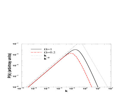
FIG. 1.: Behaviour of the power spectrum for a CDM model with $\Omega=1,0.2$ respectively. The two reference lines have exponents $k\;,k^{-2}$.

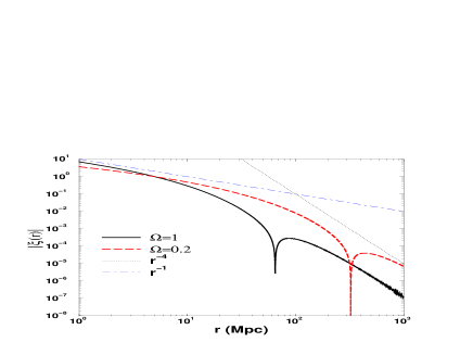
FIG. 2.: Behaviour of absolute value of the real space correlation function for the two CDM models $\Omega=1,0.2$ and $h=0.5$. The two reference lines are $r^{-4}$ and $r^{-1}$. Note that at small scale $\tilde{\xi}(r)>0$, with a zero crossing at a scale depending on the location of the peak or “turn-over” in the PS, after which it remains negative ($\tilde{\xi}(r)\sim-r^{-4}$) at larger distances. The correlation function has been normalised to be $\tilde{\xi}(r_{0})=1$ for $r_{0}=5Mpc$.

In Fig.3 we show the behaviour of the unconditional variance, computed in real-space spheres. We see again a clear convergence in both models to the predicted $1/R^{4}$ behaviour beyond the scale characterizing the “turn-over”.

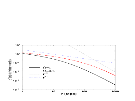
FIG. 3.: Behaviour of the unconditional variance in spheres for the two CDM models $\Omega=1,0.2$ and $h=0.5$. The two vertical lines show the transition to the $\xi(r)\sim r^{-4}$ behavior for the two models. The $r^{-4}$ behavior is a clear and distinctive feature corresponding to the $P(k)\sim k$ behavior.

In conclusion two simple real space characteristics today in the distribution of matter coming from the primordial H-Z PS are a negative non-oscillating power-law tail in the two point correlation function $\xi(r)\sim-r^{-4}$, and a $(\ln R)/R^{4}$ decay in the variance of mass in spheres of radius $R$. These are the peculiar distinctive feature of H-Z type spectra which should possibly be detected in real space by the new galaxy catalogs.

IV Real space classification of long range fluctuations

We now return to a the discussion of the nature of correlations in systems with H-Z like power spectra, with the aim of elucidating their properties by comparison with systems described in statistical physics. To this end we first introduce here a classification of all possible mass distributions in terms of the main features of the correlation function $\tilde{\xi}(r)$. Following from the discussion of Section(II) concerning the behaviour of mass fluctuations, we define three distinct classes (for either the case of discrete particle distribution and of a continuous density field):

1. If

   $$\int_{\Omega}d^{d}r\;\;\tilde{\xi}(r)=const.>0$$ (56)

   we can say that at large scale the system is substantially Poissonian. Indeed Eq. (56) implies that the PS goes to a constant non-zero value as $k$ goes to zero, and therefore that the large distance behavior of the mass fluctuations is

   $$\langle M^{2}(R)\rangle-\langle M(R)\rangle^{2}\sim R^{d}\sim\langle M(R)\rangle\,.$$ (57)

   We write here the unnormalized form of the variance, as the result that the variance of an extensive quantity such as the mass is proportional to the volume on which it is measured is the most intuitive way of characterizing a Poisson type behaviour. In this class is, for example, a system with a finite range correlation $\xi(r)\sim e^{-r/r_{c}}$. Beyond the scale $r_{c}$ (the correlation length - see below for a discussion about this length) the system is uncorrelated and effectively Poissonian.

2. If

   $$\int_{\Omega}d^{d}r\;\;\tilde{\xi}(r)=+\infty$$ (58)

   then we are in a case similar to a system at the critical point of a second order phase transition (e.g. the liquid-gas critical point). Such systems have a positive correlation function which is asymptotically a positive power law, with $\xi(r)\sim 1/r^{\gamma}$ and $\gamma<d$, corresponding to a PS $P(k)\sim k^{\gamma-d}$ as $k\rightarrow 0$. One then has at large scales the variance

   $$\langle M^{2}(R)\rangle-\langle M(R)\rangle^{2}\sim R^{\alpha}\;\;\mbox{with}\;d\leq\alpha<2d\;,$$ (59)

   or $\langle M^{2}(R)\rangle-\langle M(R)\rangle^{2}\sim\langle M(R)\rangle^{\beta}$ with $\beta=\alpha/d>1$. This means that mass fluctuations are large (always overwhelming the Poisson fluctuations) and thus they are strongly correlated at all scales. It is in this context that the concept of self-similarity and scale-invariance has been introduced in statistical mechanics. These terms refer to the fact that in these systems the mass fluctuation field has well defined fractal properties [25].

3. If

   $$\int_{\Omega}d^{d}r\;\;\tilde{\xi}(r)=0$$ (60)

   then, as we have discussed, we have for the behaviour of the mass fluctuations

   $$\langle M^{2}(R)\rangle-\langle M(R)\rangle^{2}\sim R^{\alpha}\;\;\mbox{with}\;d-1<\alpha<d\,,$$ (61)

   i.e. $\langle M^{2}(R)\rangle-\langle M(R)\rangle^{2}\sim\langle M(R)\rangle^{\beta}$ with $\beta=\alpha/d<1$, so that the mass fluctuations are always asymptotically smaller than in the uncorrelated Poisson case. This also corresponds to a strongly correlated, long-range ordered, system. We will refer to them with the term “super-homogeneous” to underline this feature that they are more homogeneous than a Poisson system. (Indeed, the Poisson particle distribution is considered as the paradigm of a stochastic homogeneous mass distribution [26]). In the context of statistical mechanics they can be described as glass-like, as they have the properties of glasses, which are highly ordered compact systems. That can be said to be typically lattice-like, with a long-range ordered packing, but without the discrete symmetries of an exact lattice. Note again that, since $\tilde{\xi}(0)>0$ (a Dirac delta function in the discrete case) by definition, $\tilde{\xi}(r)$ must change sign with $r$ at least once. They are systems with finely balanced positive and negative correlation.

The distinction between 1 and 2 is typical of the statistical physics of critical phenomena in order to distinguish a critical state (case 2) from a non-critical state (case 1). In this context the concept of correlation length is central. The correlation length is a measure of the distance up to which one has spatial memory of the spatial variations in the mass density [19]. There is no unique definition of this length scale, but from a phenomenological point of view it can be defined as the length scale up to which the effect of a small local perturbation in the system is felt. This is due to the fluctuation-dissipation theorem which links the response of the system to a local perturbation and the large scale behavior of the two-point correlation function (for the different precise definitions of the correlation length see for example [10]). A simple definition is (but see also [21, 22])

$$r_{\rm{corr}}^{2}=\frac{\int_{\Omega}r^{2}d^{d}r\;\;|\tilde{\xi}(r)|}{\int_{\Omega}d^{d}r\;\;|\tilde{\xi}(r)|}\;.$$ (62)

In case 1 one can generally define a finite correlation length, while in case 2 it will generally diverge. In particular in the case $\xi(r)\sim\exp(-r/r_{c})$, $r_{c}$ is indeed then the correlation length, while for a positive power-law $\xi(r)\sim 1/r^{\gamma}$ and $\gamma<d$ (case 2) $r_{\rm{corr}}\rightarrow\infty$.

Case 3 is typical of ordered compact systems with small correlated perturbations. One can meet this kind of correlation function for example in the statistical physics of liquids, glasses, phonons in lattices. The concept of correlation length in this context is less central, and the extension of its use to this class of systems is not particularly useful. Instead it is appropriate to classify the correlation properties of these systems directly through the integral of the correlation function as we have done. It is this behaviour of their correlations which distinguishes them from the other two cases, just as these cases are typically distinguished from one another by the value (finite or infinite) of their correlation length. Certainly, as we have noted, the use of the term “correlation length” in the cosmological literature, which is defined [14] as a scale defining the amplitude of the correlation function, is in no way related to its use in statistical physics.

Before continuing with a more detailed discussion of the nature of this class of super-homogeneous distributions to which standard cosmological models belong, we clarify one quite common misunderstanding about them in cosmology.

V $P(0)=0$ and constraints in a finite sample

As we have noted in the introduction the physical meaning of the constraint $P(0)$, equivalent to Eq. (60), is often missed in the cosmological literature because of a confusion with the so-called “integral constraint”, which is another very similar, but actually completed different, constraint. Let us clarify this point.

The “integral constraint” refers in this context to a constraint which appears in the estimation of the correlation function in a finite sample ($S$, say). It is a constraint which indeed can take the superficially similar form to (60):

$$\int_{S}d^{3}r\;\;\tilde{\xi}_{E}(r)=0$$ (63)

where the subscript indicates that the integral is over the finite sample volume, and $\tilde{\xi}_{E}(r)$ is the value of the estimator of the correlation function. This is in general a quantity calculable from the sample whose ensemble average converges to the real correlation function at any finite scale when the boundaries of the sample go to infinity.

That such a constraint has in principle nothing to do with the constraint $P(0)=0$ is clear from the fact that it is one which holds independently of what kind of distribution the sample is taken from. Its origin is simple, in the fact that the the mean mass density, relative to which fluctuations are estimated, is taken in the estimator from the sample itself. Therefore, roughly speaking, the positive correlations measured relative to this density are constrained to be balanced by anti-correlations, giving rise to a constraint like Eq. (63). More specifically the two point correlation function can be written as

$$\tilde{\xi}(r)=\frac{\langle n(r)\rangle_{p}}{\langle n\rangle}-1$$ (64)

where $\langle n(r)\rangle_{p}$ is the mean density at distance $r$ from an occupied point and $\langle n\rangle$ the true (unconditional) mean density. Integrating this expression over the volume of the sample $S$ gives the relation

$$\langle N_{S}\rangle_{p}-\langle N_{S}\rangle=\langle n\rangle\int_{S}d^{3}r\;\;\tilde{\xi}(r)$$ (65)

where $\langle N_{S}\rangle_{p}$ is the average number of points in the sample volume, with a point at the origin by construction, while $\langle N_{S}\rangle$ is the average number of points is the same volume, but without the condition that there is a point at the location of the observer. If one estimates the true mean density (i.e. $\langle n\rangle=\langle N_{S}\rangle/V_{S}$) in a galaxy catalogue sample from the actual density in the sample (i.e. on average $\langle N_{S}\rangle_{p}/V_{S}$), the estimator for the correlation function will by construction on average obey the condition Eq.(63) i.e.

$$\int_{S}d^{3}r\;\;\langle\tilde{\xi}_{E}(r)\rangle=0.$$ (66)

Such a systematic (i.e. ensemble average) offset between the estimated and the real correlation function is sometimes referred to in the cosmological literature on the subject as “bias”. It is only in very specific circumstances, with certain estimators, that Eq.(63) holds for a single sample. For an estimator of the form [25]

$$\tilde{\xi}_{E}(r)=\frac{\Gamma(r)}{n_{S}}-1$$ (67)

where $\Gamma(r)$ is estimator of $\langle n(r)\rangle_{p}$, and $n_{S}$ an estimate of the mean-density from the sample, Eq.(63) will hold if

$$n_{S}=\frac{1}{V_{S}}\int_{S}\Gamma(r)d^{3}r\;.$$ (68)

This is in fact a perfectly good prescription for how to estimate the mean density in a finite sample, but one that is not used in most estimators, which typically have a variance around the average behaviour Eq. (66). Estimators which do not take the mean density as the simple density of points in the sample do not in general obey even Eq.(66), but will always obey some constraint of this type, which cannot be avoided because it is intrinsic to the fact that any real sample contains an occupied point at the position of the observer.

In summary there are necessarily constraints on the correlation function $\tilde{\xi}_{E}(r)$ measured in a finite sample, which may take a form similar to the condition Eq. (60) defining super-homogeneous distributions, but over a finite integration volume. These two kinds of constraint have a completely different origin and meaning, one describing an intrinsic property of the fluctuations in a certain class of distributions, the other a property of the estimated correlation function of any distribution as measured in a finite sample. Their formal resemblance however is not completely without meaning and can be understood as follows: in a super-homogeneous distribution the fluctuations between samples are extremely suppressed, being smaller than poissonian fluctuations; in a finite sample a similar behaviour is artificially imposed since one suppresses fluctuations at the scale of the sample by construction. An estimator which imposes the relation Eq.(66) on the estimated correlation function would therefore be expected to make a smaller error for the class of super-homogeneous distributions than for others. We will return to issues such as this in forthcoming work.

VI Super-homogeneous Distributions

In this section we discuss the properties of long-range ordered mass distributions, or super-homogeneous distributions. We first discuss the simplest example of such a situation, represented by a lattice of particles. It has many of the relevant properties under discussion. By studying its perturbation (the “shuffled lattice”) it is possible to understand the properties of more isotropic distributions, both continuous and discrete, which are characterized again by long-range order. The main feature of these distributions, as we have discussed, is that $\sigma^{2}(R)$ (the unconditional variance) decays faster than in the uncorrelated Poissonian case, i.e. faster than $R^{-d}$(where $d$ is the space dimension). We then discuss how a continuous field with such correlations can be constructed, making it clear that the intuitions about the nature of the fluctuations in the shuffled lattice can be extended to the continuous case. We mention here that one physical model in which such correlations are found is the “one component plasma” studied, for example, in [11, 37]. This models a Coulomb system of discrete positive charges in a continuous negatively charged background. In equilibrium the charges reach an extremely ordered glass-like configuration with PS at small $k$ like that of the shuffled lattice.

A The perfect lattice

The microscopic density in the case of particles placed on the sites of a regular lattice (in any dimension) can be simply written as

$$\rho(\vec{r})=\sum_{\vec{R}}\delta(\vec{r}-\vec{R}-\vec{\eta})$$ (69)

where $\vec{R}$ is the generic lattice displacement vector and $\vec{\eta}$ is position vector of the lattice site with $\vec{R}=0$ with respect to the origin of coordinates, i.e. $\vec{R}+\vec{\eta}$ runs over all the lattice sites. For simplicity let us suppose we have a cubic lattice of unitary lattice spacing. Then, in order to eliminate the dependence on the position of the origin of coordinates with respect to the lattice, we can define an ensemble of lattices by varying the position of the origin with uniform probability in an unitary cell. For instance in $d=3$, $-1/2\leq\eta_{x},\eta_{y},\eta_{z}<1/2$ where $x,y,z$ are the axis coordinates, and then the “ensemble average” is $\left<...\right>\equiv\int\int\int_{-1/2}^{1/2}d\eta_{x}d\eta_{y}d\eta_{z}...$.

Clearly we have that

$$\langle\rho(\vec{r})\rangle=1\;.$$ (70)

We want to compute now the two-point correlation function $\langle\rho(\vec{r}_{1})\rho(\vec{r}_{2})\rangle$. Firstly we have that

$$\rho(\vec{r}_{1})\rho(\vec{r}_{2})=\sum_{\vec{R}_{1},\vec{R}_{2}}\delta(\vec{r}-\vec{R}_{1}-\vec{\eta})\delta(\vec{r}-\vec{R}_{2}-\vec{\eta})\;.$$ (71)

from which one obtains

$$\langle\rho(\vec{r}_{1})\rho(\vec{r}_{2})\rangle=\sum_{\vec{R}}\delta\left(\vec{r}_{1}-\vec{r}_{2}-\vec{R}\right)$$ (72)

and hence the two-point correlation function

$$\tilde{\xi}(\vec{r}_{1},\vec{r}_{2})=\frac{\langle\rho(\vec{r}_{1})\rho(\vec{r}_{2})\rangle}{\langle\rho\rangle^{2}}-1=$$ (73)

$$\!\left(\!\sum_{\vec{R}}\delta(\vec{r}_{1}-\vec{r}_{2}-\vec{R})\right)\!\!-\!1\;.$$ (74)

Note that $\tilde{\xi}(\vec{r}_{1},\vec{r}_{2})\equiv\tilde{\xi}(\vec{r}_{1}-\vec{r}_{2})$ which means that our occupation stochastic process (i.e. the ensemble) is stationary. However since it is not invariant for generic spatial rotations we have $\tilde{\xi}(\vec{r}_{1}-\vec{r}_{2})\neq\tilde{\xi}(|\vec{r}_{1}-\vec{r}_{2}|)$ (the lattice breaks spatial isotropy).

In order to evaluate $P(\vec{k})$ we need to perform the FT of $\tilde{\xi}(\vec{r})$. In the case of a lattice this gives simply

$$P(\vec{k})=\sum_{\vec{h}\neq 0}\delta(\vec{k}-\vec{h})$$ (75)

where the sum is extended to all the dual lattice vector $\vec{h}$ satisfying the duality condition $\vec{h}\cdot\vec{R}=2\pi m$, where $m$ is any integer, but with the exception of $\vec{h}=\vec{0}$. Note that, because of this last condition, also in this case $P(\vec{0})=0$.

It has been shown [16] that for the simple lattice in $d$ dimensions the fluctuations in a ball of radius $R$, centered on a randomly chosen point, behaves as

$$\langle M(R)^{2}\rangle-\langle M(R)\rangle^{2}\sim R^{d-1}.$$ (76)

compared to the Poisson behaviour $\langle M(R)^{2}\rangle-\langle M(R)\rangle^{2}\sim R^{d}$. This result can be understood as follows:

• In the Poisson distribution, if we take two randomly placed spheres of same radius, the numbers of particle contained in them differ by an amount which is typically of the order of the square root of the average number ($\sim R^{d}$);

• In the case of a lattice the two numbers differ by an amount which corresponds to a Poissonian fluctuation (i.e. the square root) of the number of particles contained in the last shell of the sphere of thickness equal to the lattice spacing (which scales as $R^{d-1}$).

This is due to the strong order of the particles in the lattice from a large scale point of view. Thus the lattice has a behaviour of its mass variance which places it in the super-homogeneous category, with the limiting decreasing behaviour

$$\sigma^{2}(R)\sim R^{-(d+1)}\;,$$ (77)

i.e. $\sigma^{2}(R)\sim R^{-4}$ for $d=3$.

B The “shuffled” lattice

In this section we define a super-homogeneous stochastic distribution of particles obtained from a lattice which shows more evident resemblances with the cosmological H-Z case. The recipe is the following: 1) Consider a cubic lattice of particle, as discussed above; 2) take a particle of the distribution and draw a lattice-oriented cubic box of size $l$ larger than the lattice spacing centered on the particle itself; 3) displace the particle to a randomly chosen point of this box; 4) repeat for each particle of the lattice.

We can write $\rho(\vec{r})$ for a certain realization of this stochastic process as

$$\rho(\vec{r})=\sum_{\vec{R}}\delta(\vec{r}-\vec{R}-\vec{\eta}_{\vec{R}}-\vec{\eta})\,,$$ (78)

where $\vec{R}$ and $\vec{\eta}$ have the same meaning as before, and $\vec{\eta}_{\vec{R}}$ is the vector giving the displacement of the particle in the box from the lattice rest position $\vec{R}+\vec{\eta}$. By definition each component of the vector $\vec{\eta}_{\vec{R}}$ is a random number uniformly distributed in the interval $[-l/2,+l/2]$. Therefore, for instance in $d=3$, the ensemble average $\left<...\right>$ is now defined to be:

$$\left<...\right>=\int\int\int_{-1/2}^{1/2}d^{3}\eta\prod_{\vec{R}}\int\int\int_{-l/2}^{l/2}\frac{d^{3}\eta_{\vec{R}}}{l^{3}}...\;.$$ (79)

After some algebra one finally obtains that $\tilde{\xi}(\vec{r}_{1},\vec{r}_{2})\equiv\tilde{\xi}(\vec{r}_{1}-\vec{r}_{2})$ (i.e. the ensemble is stationary) and in $d$ dimensions for integer $l$ one finds exactly:

$$\tilde{\xi}(\vec{r})=\delta(\vec{r})-\prod_{k=1}^{d}\left\{\begin{array}[]{ll}\frac{1}{l}-\frac{|r_{k}|}{l^{2}}\;\;\mbox{if}\;\;|r_{k}|<l\\ 0\;\;\mbox{if}\;\;|r_{k}|\geq l\end{array}\right.\;.$$ (80)

It is very simple to verify that $\int\int\int_{-\infty}^{\+\infty}\tilde{\xi}(\vec{r})d^{3}r=0$, which is the condition of super-homogeneity. Note that for $l\rightarrow+\infty$ $\tilde{\xi}(\vec{r})$ reduces correctly to the simple delta function, i.e. to the Poisson correlation function. In fact in that limit we must of course obtain a Poissonian distribution of particles without correlations. Note that consequently, we have the following non-commutativity of the limits:

$$0=\lim_{l\rightarrow\infty}\int\int\int_{-\infty}^{\+\infty}\tilde{\xi}(\vec{r})\neq\int\int\int_{-\infty}^{\+\infty}\lim_{l\rightarrow\infty}\tilde{\xi}(\vec{r})=1\,.$$ (81)

One can also find an exact form of $P(\vec{k})$ by applying Eq.(34) in $d$-dimensions:

$$P(\vec{k})=\frac{1}{(2\pi)^{d}}\left[1-\prod_{i=1}^{d}\frac{2(1-\cos(l\,k_{i}))}{l^{2}\,k_{i}^{2}}\right]\,.$$ (82)

Let us analyze the behavior for small values of $k$. At the leading order we can write

$$P(\vec{k})\approx\frac{l^{2}}{(2\pi)^{d}}\frac{k^{2}}{12}\,,$$ (83)

which implies an isotropic behavior for $k\rightarrow 0$ even though by construction $P(\vec{k})$ is not isotropic for a general $\vec{k}$. Note that we have the $P(\vec{0})=0$ behaviour of the H-Z spectrum. Finally, the fact that for $k\rightarrow\infty$ the PS tends to a positive constant, means that such a distribution is Poissonian at small scale ($r<l$).

It is now easy to calculate analytically the unconditional number variance. In particular the calculation can be done exactly in cubic boxes with the same lattice symmetry and, with some simple approximations, in spheres. In both cases one obtains $\sigma^{2}(R)\sim R^{-4}$ for large scales, as in the case of a lattice, but eliminating the pathology of different scaling behaviors between cubic boxes and spheres which we noted is present for the rigid lattice. Note that the fact that $\sigma^{2}(R)\sim R^{-4}$ at large scales corresponds to the fact that, despite the “shuffling” of particles with respect to the lattice, the strong lattice order is maintained at large scales. For non-integer $l>1$ , even though calculations are cumbersome and $\xi(r)$ is not simply writtable, the main results about $P(k)$ for small $k$ and $\sigma^{2}(R)$ for large $R$ are the same.

The H-Z spectrum has this same behaviour characteristic of lattice-like order at large scales, while its small $k$ PS is $P(k)\sim k$ instead of $\sim k^{2}$. This spectrum corresponds to more power at large scales. We will see in the next section that this can be associated with an appropriately more ordered (i.e. coherent) shuffling of the lattice, and precisely what kind of large scale correlations is required to obtain the H-Z spectrum will be made explicit. The crucial point is that such shuffling must leave intact at very large scales the strong order of the lattice, so that one still has the characteristic behaviors we have seen in the shuffled lattice (a correlation function which is negative at large scales and integrates to zero, a normalised variance in spheres decreasing faster than the volume). We thus say that the distribution described by the H-Z spectrum has a lattice-like or, more appropriately because of the isotropy, glass-like long range order. More specifically it can be characterized as a glass with superimposed opportune coherent long-range perturbative waves of displacement.

In relation to this description it is interesting to make some brief comments on cosmological N-body simulations (see e.g.[6]). In this context a standard algorithm used to generate initial conditions for these simulations involves imposing perturbations on a perfect lattice (or sometimes even “glassy” configuration). At first sight this would suggest that the point we are making about the H-Z spectrum is in fact already understood in the cosmological literature, or at least in the part of it on N-body simulations. This is not the case, and it is worth explaining this to avoid any possible confusion on this point. This technique for generating initial conditions has in fact been introduced to avoid problems with Poisson noise at small scales (large $k$) in the discretization procedure, and not because the system being simulated is understood to actually intrinsically resemble a lattice at small $k$. Indeed the primary goal of most of these simulations has been to study the dynamical evolution in a range of scales well below the “turn-over” in the PS, where the PS (at large $k$) has a negative power-law form ($\sim k^{-\beta}$, with $\beta>0$, corresponding to a positive correlation function with a “critical” power law behaviour). Thus this procedure is applied primarily in a range of scales where the system being modeled does not intrinsically resemble a lattice or glass at all.

Only the more recent very large simulations describe the larger scales at which the initial conditions should have $P(k)\sim k$. In this case too the use of a displaced lattice in setting up initial conditions is not because the underlying system is understood to be lattice-like, but is simply inherited as a numerical technique for the same small scale considerations [30]. Indeed, as will be further clarified in the following section, there is in principal no reason why one has to start from a lattice to produce such a spectrum; nor indeed is it certain that one obtains the right correlation properties if one starts from a lattice. What is true is that the spectrum of the initial conditions, if it is H-Z, should be glass-like in the sense we have discussed. A real space analysis of the initial conditions actually used in such simulations shows [7] that they do not in fact have the appropriate properties.

Note finally that glass-like systems belong to a wide family of distributions for which the common feature is that $P(k)\sim k^{a}$ with $a>0$ for $k\rightarrow 0$ and hence $P(0)=0$. However such behaviors in the PS do not imply directly that $\xi(r)$ has a negative power-law tail at large scales. In particular this is not true if the PS has a singularity for $P(0)\neq 0$, as happens in many systems. For example [7] the glass-like distributions (unperturbed and perturbed) used as initial conditions in cosmological N-body simulations have indeed an oscillating $\xi(r)$ at all scales, and a mass variance $\sigma^{2}(r)\sim r^{-4}$. Thus we emphasize that the negative power-law tail of the real-space correlation function of the H-Z distributions in cosmology is a very particular feature of these models.

C Uniform distributions with a displacement field

Let us consider the case of a mass distribution (a density field) obtained by superimposing a random displacement field on a completely uniform density field.

Let the uniform density field be $\rho_{0}(\vec{r})=\rho_{0}$ and superimpose on it the stochastic displacement field $\vec{u}(\vec{r})$ (the infinitesimal volume $dV$ at $\vec{r}$ is displaced by $\vec{u}(\vec{r})$). Let us call $\rho(\vec{r})$ the resulting density field. We suppose that the stochastic field displacement is the realization of a stationary and isotropic stochastic process characterized by the probability density functional ${\cal P}[\vec{u}(\vec{r})]$. In this way ${\cal P}[\vec{u}(\vec{r})]$ defines also an ensemble of density fields $\rho(\vec{r})$ which is stationary and isotropic, with $\left<...\right>$ the ensemble average.

By applying the mass conservation (i.e. the continuity equation) we find

$$\frac{\rho(\vec{r})-\rho_{0}}{\rho_{0}}\simeq-\vec{\nabla}\cdot\vec{u}(\vec{r})\,.$$ (84)

If we call as usual $\xi(r)$ the reduced two-point correlation function of the density field we can write

$$\xi(r)=\left<\vec{\nabla}\cdot\vec{u}(\vec{r})\vec{\nabla}\cdot\vec{u}(\vec{0})\right>\,.$$ (85)

Then, taking the FT of both sides of Eq. (85), and making use of the statistical isotropy, we obtain

$$P(k)\sim k^{2}P_{u}(k)\,,$$ (86)

where $P(k)$ is the usual PS of the mass density field and $P_{u}(k)$ is the PS of the displacement field.

Since $P_{u}(k)$ is a itself the PS of a SSP it is subject to the constraints of the Khintchine theorem. Thus at small $k$ it must diverge slower than $\sim k^{-3}$, allowing to obtain at most $P(k)\sim k^{-1}$, corresponding to a real space correlation function which must go to zero faster than $1/r^{2}$ as $r\rightarrow\infty$. Therefore any continuous SSP of the “substantially Poissonian” and “super-homogeneous” type can be obtained in this way, but not all the “critical” type behaviors. In particular one can obtain a H-Z type spectrum with $P_{u}(k)\sim k^{-1}$ describing a critical type SSP.

What is the relation to the discrete case? If we suppose that $P_{u}(0)=const.>0$, i.e. the displacement field at large spatial scales is Poissonian (i.e. uncorrelated), we find that for $k\rightarrow 0$ one has $P(k)\sim k^{2}$. This is exactly the same asymptotic behaviour as that we found for the case of the shuffled lattice. Indeed we obtained the latter through the superposition of an uncorrelated random displacement field to a “uniform” background, and thus the result is natural. Moreover in general we would expect the relation Eq. (86) to give us in the discrete case the large scale behaviour of a set of fluctuations imposed on a discretization of the continuous uniform density field, and in particular of a rigid lattice which is simply such an object. Thus if instead of shuffling the lattice as in the previous section we superimpose correlated fluctuations with a spectrum $\sim k^{-1}$ we will obtain at large scales a distribution with H-Z behaviour, and the associated real space properties at large scales.

Let us return again finally to our comments at the end of the last section on N-body simulations (see [7] for a more complete discussion of this point). With the previous construction it is easy to see why one arrives at the idea of generating a distribution with a certain PS by displacing points on a rigid lattice. The lattice is simply a discretization of the continuous uniform background which is then perturbed. One could in principle start from a Poissonian distribution of particles - for the generation of the large $k$ behavior - which can be always made “uniform” to any desired precision (assuming no practical limitation on the number of points used), and then superimpose the displacement field to produce the required PS. If the distribution produced is to be H-Z, and particluary of CDM type, it will have the “super-homogeneity” of a lattice at the corresponding scales, with the characteristic real space behaviors we have used to define it. Equally if one starts from a lattice one can arrive at distributions which are not super-homogeneous. Indeed, as we noted above, in the context of N-body simulations in cosmology the displacement from a lattice to produce initial conditions has been introduced in simulations describing the evolution in cosmological models at scales where the models are not H-Z, but rather have a positive correlation function with a “critical” power-law. The starting point of a lattice has been favored over a “uniform” Poisson distribution simply because of numerical limitations, the latter producing at any feasible resolution too much small scale noise overwhelming correlations at small scales. In summary the central point we are making here is not that a H-Z type spectrum can be obtained in principal by perturbing a lattice; rather the crucial point is that such a system is intrinsically lattice-like, irrespective of how a discrete realization of it is constructed in practice. These are two completely different things.

VII Discussion and Conclusions

First we return to the use of several terms “scale-invariance” in cosmology. We have described in section(III) with what meaning this term has been introduced in cosmology: it refers to the fact that the variance of the mass (or equivalently gravitational potential) has an amplitude at the horizon scale which does not depend on time. The PS associated with this behaviour is that of a correlated system which is of the super-homogeneous type. This use of the term “scale-invariance” therefore is not in any way analogous to its (original) use in statistical physics. In this context it is associated with a distinctly different class of distributions which have special properties with respect to scale transformations: typically critical systems, like a liquid-gas coexistence phase at the critical point, which have a well defined homogeneity scale and a reduced two-point correlation function which decays as a non-integrable power law: $\xi(r)\sim r^{-\gamma}$ with $0<\gamma<3$. In particular the term does not have anything to do with the amplitudes of fluctuations being independent of scale: the amplitudes of fluctuations vary with scale, while the system is correlated at all scales.

We note that one might be tempted to associate the term “scale-invariance” in the context of cosmology simply to the power-law behaviour of the correlation function. From a mathematical point of view, the terminology “scale-invariance” could be used for any distribution with a power-law tailed $\xi(r)$, that is satisfying $\xi(r^{\prime})=A(b)\xi(r)$ for $r^{\prime}=br$ . In this case the H-Z spectrum would, however, be no more “scale-invariant” than any other spectrum with a power-law form at small $k$. In terms of its meaning in physics however this usage is restricted to the context of critical phenomena, in which it has been demonstrated to be very powerful and useful. As we have discussed, this case is completely different from the systems we have termed super-homogeneous. In particular in the former systems fluctuations are always large at all scales, which formally is associated with the non-integrability of the correlation function. The super-homogeneous systems have correlations of a completely different kind: they are delicately balanced to make the mass fluctuations smaller than for a Poisson type distribution.

In section (IV) we have briefly discussed the use of the term “correlation length”. Historically this term was introduced in the context of critical phenomena to characterize the transition towards a state of the system where (positive) correlations are long range and the normalized fluctuations of the mass (or of other extensive quantities) decay with the scale more slowly than in the non-critical Poissonian state. Moreover in this context, the meaning of correlation length is given through the fluctuation-dissipation theorem, in which the correlation length plays the role of the distance up to which the system responds to a local external perturbation. It is thus a scale used to capture the essential physical distinction between two types of distributions which are both in turn distinct from the superhomogeneous systems. The essential difference between each of these three cases can be best characterized according to the large scale behavior of the mass fluctuations in each case. It is therefore useful to take as classification parameter the value of the integral of $\tilde{\xi}(r)$ over all space as we have done, while the notion of correlation length has no obvious or unique generalization in this case.

Another term whose meaning it is useful to clarify is “fractal”. Fractal distributions, which are the prototype of scale-invariant geometrical distributions, represent a more extreme case of correlated systems: their average density is zero in the infinite volume limit and the conditional average density $\left<n(\vec{r})\right>_{p}$ decays to zero as a power law $r^{-\gamma}$ as a function of the distance from an occupied point (with $0<\gamma<d$). The fractal dimension of the mass distribution is given by $D_{f}=d-\gamma$ [38, 39]. A fractal is inhomogeneous at all scales and the concept of average density in a finite sample centered on an occupied point has no intrinsic meaning, because it depends on the sample size. Moreover, since the asymptotic average density of a fractal distribution is zero, both $\xi(r)$ and $P(k)$ are undefined for such a system [25]. Instead one has to work directly with the unnormalized conditional density $\left<n(\vec{r})\right>_{p}$. In general, before introducing the estimators of $\xi(r)$ and $P(k)$ for a finite sample of a system whose underlying properties one does not know (e.g. the distribution of galaxies in the Universe), one needs to verify that the estimator of the average density $\rho_{0}$ is not strongly dependent on the sample size [25].

There is sometimes confusion in the cosmological literature about the meaning of “fractal” in connection with the notion of scale invariance. For example in the book by Peacock [40] (Sect.16) the author writes that “The Zeldovich spectrum is a scale-invariant spectrum….”. It is then shown that the PS of the fluctuations in the gravitational potential $P_{\phi}\sim k^{-3}$ and hence the auto-correlation function, or the quantity $\Delta_{\phi}^{2}\sim P_{\phi}(k)\cdot k^{3}$ is a constant: the author concludes that “Since potential perturbations govern the flatness of space-time, this says that the scale-invariant spectrum corresponds to a metric that is fractal : space-time has the same degree of ‘wrinkliness’ of each resolution scale.” Both the term “fractal” and “scale-invariance” are used here in an incorrect and misleading way with respect to any of the meanings attached to them in their (original) context of statistical physics. In particular the H-Z spectrum does not have any properties which would allow it to be associated with a fractal mass distribution.

We have discussed the criterion which leads to the H-Z spectrum. We have pointed out that the usual naive formulation of this condition is in fact not satisfied by the spectrum $P(k)\sim k$, and that one must phrase the condition in terms of the variance in Gaussian spheres at the scale of the horizon. This is because the spectrum $P(k)\sim k$ is singled out by the constancy (as a function of time) of $k^{3}P(k)$ at the horizon scale, which cannot be taken to be proportional to the variance in spheres of radius $R\sim k^{-1}$ for $P(k)\sim k^{n}$ and $n\geq 1$. We have emphasized that this is not at all an unphysical behaviour due to the ideality of a sphere. Rather it actually tells us something very fundamental about the nature of these distributions: They are distributions which are so ordered at large scales that the variance of mass at large scales really does come from small scales. The H-Z spectrum marks the transition to a pure lattice-like behaviour of the normalised variance in spheres $\sigma^{2}(R)\sim 1/R^{4}$, which has been shown to be the most rapid possible decay of this quantity for any stochastic distribution of points.

What then does the use, widespread in cosmology, of a Gaussian sphere mean for such a distribution? Mathematically it simply filters out the power up to a certain mode $k$ (which then dominates the integral). Physically it can be extremely misleading if interpreted incorrectly as a characterization of a variance in real space. Consider the example of the shuffled lattice. It has PS $\sim k^{2}$ at small $k$ (i.e. $kl\ll 1$, where $l$ is the shuffling scale). Using a Gaussian sphere one would infer that the variance at large scale goes as $1/R^{5}$. Physically we know that all the variance comes from small scales in this case, and that this behaviour dominated by the lower cut-off gives $\sigma^{2}(R)\sim 1/R^{4}$. The behaviour in Gaussian spheres comes from the fact that one is smearing the small scale behaviour over the scale $k^{-1}$. As the sphere grows the lower cut-off grows too. One would obtain the same behaviour by taking a different smearing scale on the sphere’s boundary, but by making this scale change in proportion to the radius of the sphere. The behaviour observed has to do with the very particular way one is smearing, and the real space properties of the system are actually obscured. The only usefulness of the Gaussian sphere is an alternative way of saying that $P(k)\sim k^{2}$, i.e. as a statement about $k$ space properties, not real space ones. It does not describe in any useful way a property of the system in real space. In particular the H-Z criterion should be understood really as a $k$ space one, and caution should be applied to its formulation as “constancy of mass variance at the horizon scale”.

We have highlighted the fact that all current cosmological models will share at large scales the characteristic behaviour in real space of the H-Z spectrum. Specifically we note primarily the very characteristic lattice-like behaviour of the variance in spheres $\sigma^{2}(R)\sim R^{-4}$ (up to a small correction which is formally logarithmic for the case of exact H-Z), as well as the characteristic negative (non-oscillating) power-law tail in the two point correlation function $\xi(r)\sim-r^{-4}$. In this paper we have not addressed practical questions concerning the observation of such behaviour in cosmological data. In particular one would expect such behaviour to be seen in principle, if these models are correct, in the distribution of matter in the Universe at large scales, and in particular in the distribution of galaxies. So far such behaviour has not been observed. Rather the characteristic feature of galaxy clustering at small scales is that it shows fractal behaviour [25, 41], which as we have noted corresponds to a very different kind of distribution than that described by CDM type models. A centrally important (and much debated [25, 41, 24]) observational question is the determination of the scale marking the transition from this behaviour to homogeneity. On much larger scales galaxy structures should then present the super-homogeneous character of the H-Z type PS. Indeed this should be a critical test of the interpretation of measurements of CMBR in terms of the H-Z picture on large spatial scales [4, 34, 35]. Observationally a crucial question is the feasibility of measuring the transition between these regimes directly in galaxy distributions. With large forthcoming galaxy surveys it may be possible to do so, but this is a question which must address exactly the statistics of these surveys and the exact nature of the signal in any given model. These are questions we will address in future works. One other direct usage of the results developed here is in the context of N-body simulations, in which one studies numerically the evolution of perturbations in cosmological models, and a knowledge of their real space characteristics can be very useful. We refer to [7] for a detailed discussion of this point.

REFERENCES

- [1] P. J. E. Peebles, Principles Of Physical Cosmology, (Princeton University Press, 1993).
- [2] E.R Harrison, Phys.Rev. D 1, 2726 (1970).
- [3] Ya.B. Zeldovich, Mon.Not.R.Acad.Soc. 160, 1 (1972).
- [4] C.L. Bennett et al., Astrophys.J., 436, 423 (1994)
- [5] G. Efsthathiou, M. Davis, C. Frenk and S. White, Astrophys.J.Suppl. 57, 241 (1985)
- [6] A. Jenkins et al., Astrophys.J. 499, 20 (1998)
- [7] T. Baertschiger & F. Sylos Labini, Europhys Lett. to appear (2002), astro-ph/0109199
- [8] S. Chandrasekhar, Rev. Mod. Phys. 15, 1 (1943)
- [9] A. Gabrielli, F. Sylos Labini and S. Pelligrini, Europhys Lett. 46, 127 (1999)
- [10] S.K. Ma The Modern Theory of Critical Phenomena (Benjamin Reading, 1976)
- [11] D. Levesque, J.-J. Weis and J. L. Lebowitz, Journal of Statistical Physics 100, 209 (2000)
- [12] Padmanabhan T., Structure formation in the universe (Cambridge University Press, 1993)
- [13] E.W. Kolb and M.S. Turner, The Early Universe (Addison-Wesley Publishing Company, 1990)
- [14] P.J.E Peebles, Large Scale Structure of the Universe (Princeton Univ. Press, 1980)
- [15] W.C. Saslaw, The distribution of galaxies (Cambridge University Press, 2000)
- [16] D. G. Kendall and R. A. Rankin, Quart. J. Math. Oxford (2) 4, 178 (1953)
- [17] J.L. Doob, Stochastic Processes (John Wiley & Sons, New York, 1953)
- [18] A. Gabrielli & F. Sylos Labini, Europhys.Lett. 54, 1 (2001)
- [19] K. Huang, Statistical Mechanics (Jonh Wiley & Sons, New York, 1987)
- [20] L.D. Landau and E.M. Lifshitz, Statistical Physics (Mir Moscow, 1978)
- [21] J. Gaite, A. Dominuguez and Perez-Mercader J., Astrophys.J.Lett. 522, L5 (1999)
- [22] A. Gabrielli, F. Sylos Labini and R. Durrer, Astrophys.J. Letters 531, L1 (2000)
- [23] M. Davis, P. J. E. Peebles, Astrophys. J., 267, 46 (1983)
- [24] M. Joyce and F. Sylos Labini, Astrophys.J.Lett. 554, L1 (2001)
- [25] F. Sylos Labini, M. Montuori and L .Pietronero, Phys.Rep.,293 ,66 (1998)
- [26] W. Feller, An Introduction to Probability Theory and its Applications, Vol. 2 (Wiley & Sons New York, 1977)
- [27] Lucchin F. and Coles P., Introduction to Comsology (John Wiley & Sons, New York, 1997)
- [28] J. Beck, Acta Mathematica 159, 1-878282 (1987).
- [29] A. Liddle and D. Lyth, Cosmological Inflation and Large-Scale Structure, (Cambridge University Press, 1999).
- [30] S.D.M. White, Lectures given at Les Houches astro-ph/9410093(1993)
- [31] I. Zehavi et al., Astrophys.J submitted astro-ph/0106764 (2001)
- [32] J. A. Peacock et al., Nature, 410, 169 (2001)
- [33] D.J. Eisenstein and W. Hu, Astrophys.J. 496, 605 (1998)
- [34] P. De Bernardis et al., Nature 404, 955 (2000)
- [35] S. Hanany et al., Astrophys.J 545, L1 (2000)
- [36] M. Kershcer, I. Szapudi and A. Szalay, Astrophys.J 535, L13 (2000)
- [37] B. Jancovici, Phys. Rev. Lett. 46, 366 (1981)
- [38] B. Mandelbrot, The Fractal Geometry of Nature (Freeman, New York 1982)
- [39] K. Falconer, Fractal geometry (J. Wiley & Sons, New York, 1990)
- [40] J.A. Peacock, Cosmological Physics (Cambridge University Press, 1993)
- [41] K.K Wu, O. Lahav and M. Rees, Nature, 225, 230 (1999)