Gravitational microlensing of stars with transiting planets

If planetary systems are ubiquitous then a fraction of stars should possess a transiting planet when being microlensed. This paper presents a study of the influence of such planets on microlensing light curves. For the giant planets recently identified, the deviations in the light curve can be substantial, although the specifics of the perturbations are dependent upon the radius of the planet relative to that of the star, the location of the planet over the stellar surface and the orientation of the sweeping caustic. Given that the instantaneous probability of transiting hot-Jupiter like planets is small, less than a percent, and only a proportion of microlensing events exhibit caustic crossing events, the probability of detecting a transiting planet during a microlensing event is small, $\sim 10^{-6}$. However, a number of factors influencing this probability, such as the number of solar type star that possess planets, are uncertain, and the prospect of detecting transiting planets in future large catalogues of microlensing light curves may be viable. The results of this study also have bearing on the gravitational microlensing of spots on the stellar surface.

1 Introduction

More than fifty planets have now been identified outside the Solar system (see http://exoplanets.org for a summary of the known planetary systems). While the majority of these have been found via the measurement of a stellar radial velocity changes due to the presence of an orbiting planet, more recently the dimming of stellar light due to the transit of a giant planet has been observed, specifically in the case of HD209458 (Charbonneau et al. 2000; Henry et al. 2000; Queloz et al. 2000; Castellano et al. 2000; Doyle et al. 2000; Gaudi 2000). Typically, light curves are seen to dip by $1-2\%$ as the planet transits the star, corresponding to planetary radii of $0.10-0.14\ R_{s}$. Given current observational limits, these techniques can only be used to identify planets within a few tens of parsecs.

Gravitational microlensing has the potential to discover planets over a much greater distance. Perturbing the magnification distribution, and hence the form of the microlensing light curve, planets can be identified orbiting compact objects in the Galactic Halo (Mao & Paczyński 1991; Gould & Loeb 1992; Bolatto & Falco 1994; Bennett & Rhie 1996; Wambsganss 1997). More recently, Graff & Gaudi (2000) and Lewis & Ibata (2000) turned their attention to using gravitational microlensing to identify planets orbiting stars in the Galactic Bulge, that is detecting planets orbiting the source star in a microlensing event, rather than orbiting the lens. Assuming that the star plus planet system is swept by a fold caustic formed by a binary lens, it was shown that the feeble light that is reflected from the planet ${\rm(up\leavevmode\nobreak\ to\sim 10^{-4}L_{*})}$ can be magnified to observable levels, resulting in a $\delta M\sim 0.03$mag fluctuation. The scattering responsible for reflecting the stellar light from the planet also acts to polarize it and Lewis & Ibata (2000) demonstrated that this signature too is boosted to observable levels, probing the physical conditions in the planetary atmosphere. Following these initial studies, Ashton & Lewis (2001) considered the influence of the planetary phase on the form of the microlensing light curve, finding that when the planet appears crescent-like, the magnification can be substantially greater than the simple, circularly symmetric model that was employed in these earlier studies. While the resulting flux is still lower than that of a microlensed planet at opposition, this additional magnification does aid detection of crescent-like planets.

This paper also focuses on the identification of planets orbiting stars that are the sources during gravitational microlensing events. Instead of looking at the reflected light, however, this paper examines what effect a planet transiting a stellar surface has on a microlensing light curve. Section 2 presents simulations of such microlensing situations, considering first a simple model with a star and static planet (Sect. 2.2), while Sect. 2.3 this study is expanded to include the effects of planetary motion. Section 3 compares the results of this study with previous investigations of the influence of spots on the stellar surface, as well as investigating the frequency of planetary transits during microlensing events. Section 4 presents the conclusions of this study.

Figure 1: A sample binary caustic-crossing microlensing light curve, showing the very sharp features characteristic of a caustic crossing. This paper concerns itself only with the high magnification regions of the light curve, where the caustic actually sweeps across the source. This is highlighted in the inset box. The time scale of the microlensing event is discussed in Sect. 2.3.

2 Simulations

2.1 Microlensing

A wealth of information has resulted from the rapid growth in the field of Galactic and Local Group gravitational microlensing over the last decade. The reader is directed to the review of Paczyński (1996) which covers this background material in detail.

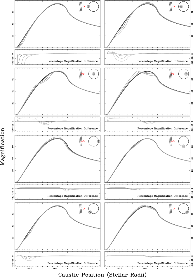
Figure 2: The microlensing light curves for the planetary configurations described in the text. In each panel, the relative position of the star, caustic (hashed region being the region of high magnification, with the arrow denoting its direction of travel) and planets are presented in the top right hand corner. Each series of light curves in a particular panel are for a range of planetary radii (0.035, 0.1, 0.2 & 0.3 $R_{s}$), the greyscale for each light curve corresponding to the greyscale of the planet in the upper portion of each figure. These light curves should be compared to the exampled light curve given in Fig. 1. The lower section of each panel presents the percentage difference in the magnification between a star with a transiting planets and the same star without such a planet. The units on the abscissa denote the position of the caustic in stellar radii, relative to the centre of the star at the origin. The total observed duration of such caustic crossings is $\sim$10 hours.

Most studies of Galactic halo microlensing have focused upon microlensing by isolated compact objects, which display simple, bell-shaped light curves. A fraction of events, however, display several rapid, asymmetric features which are characteristic of microlensing by a binary system (Alcock et al. 2000), presented schematically in Fig. 1. These features are the result of the presence of extended caustics which are associated with binary lenses. The large magnifications which result when a caustic sweeps across a source has proved to be a powerful diagnostic of not only stellar systems (Agol 1996; Han, Park, Kim & Chang 2000; Heyrovský, Sasselov & Loeb 2000), but also, at high optical depths, structure at the heart of quasars (Wambsganss & Paczyński 1991; Lewis & Belle 1998; Agol & Krolik 1999; Belle & Lewis 2000). Caustics in such networks are comprised of ‘ fold catastrophes’ (Schneider, Ehlers & Falco 1992), combining in regions to form higher order catastrophes. As they dominate the caustic structure formed by a binary lens in the following analysis it is assumed that the source star and planet are swept by a fold caustic. It is assumed that the caustic is straight in the vicinity of the source star and planet. It should be noted, however, that for a small number of microlensing light curves the observed variations are are consistent with the source star being swept with cusp-like caustics (see Alcock et al. 2000). Due to their curvature, microlensing events due to cusp caustics can result in different light curves (Fluke & Webster 1999).

As a point source is swept by a fold caustic, the magnification at a location $x$ is given by

$$\mu(x)=\sqrt{\frac{g}{x-x_{c}}}H(x-x_{c})+\mu_{o}\ ,$$ (1)

where $\sqrt{g}$ is the “strength” of the caustic, $x_{c}$ is the location of the caustic and $H(x)$ is the Heaviside step function. The background magnification, $\mu_{o}$, is due to other lensed images, not associated with the caustic crossing, formed by the binary lens. In the following study it is assumed that $\mu_{o}=1$.

An examination of Equation 1 reveals that as the caustic crosses the point source, where $x-x_{c}=0$, the resulting magnification is infinite. With any finite source, however, integrating the magnification distribution over the source results in a finite magnification, smoothing out the microlensing light curve in the vicinity of the caustic (see inset box in Fig. 1). The peak magnification in the light curve for a source swept by a fold caustic is given by

$$\mu_{peak}=f\sqrt{\frac{g}{R_{s}}}$$ (2)

where $R_{s}$ is the radius of the source, and $f$ is a form factor that accounts for the specific geometry of the source (Chang 1984). For a uniformly bright circular source, $f=1.39$. With regards to the work presented in Sect. 2.2, these parameters are chosen such that $\mu_{peak}\sim 70$, a value typical for microlensed stars of a Solar radius in the Galactic Bulge (Lewis & Ibata 2000). The results in this paper are simply scalable to other stellar radii and caustic strengths using Equation 2.

2.2 Idealized Simulations

The magnification of a star during a gravitational microlensing event is a powerful probe of the physical conditions of the stellar surface (Minniti et al. 1998; Gaudi & Gould 1999; Heyrovský, Sasselov & Loeb 2000). One particular observational success in this regard is the study of Albrow et al (1999b) who measured the limb-darkening of K giant star, the source of the microlensing event 97-BLG-28. Such a measure is only possible because the details of the surface brightness of the source star influences the form of the light curve during a gravitational microlensing event. As all stars will be limb-darkened to some degree, resulting in slightly different light curves. Hence, limb-darkening is introduced by modeling the surface brightness of the star to be (Albrow et al. 1999a; Afonso et al. 2000)

$$S(R)=1-\Gamma\left[1-\frac{3}{2}\sqrt{\left(1-\frac{R^{2}}{R_{s}^{2}}\right)}\right]$$ (3)

where $\Gamma$ is a limb-darkening parameter, such that $\Gamma=0$ corresponds to a star with a uniform surface brightness, while $\Gamma=1$ the star is centrally bright, fading to zero at $R_{s}$. Outside the range $0\leq\Gamma\leq 1$ the surface brightness distribution possesses negative regions and is, therefore, unphysical. In the following, the surface brightness of the star is parameterized with a limb-darkening of $\Gamma=0.3$, which is approximately the mean value found for the microlensing event 98-SMC-1 (Afonso et al 2000), although it is found that, while the form of the microlensing light curve is strongly dependent upon the value of $\Gamma$, the magnitude of the influence of a transiting planet is not.

The planet is also represented as a circular disk that completely obscures a fraction of light from the star. Four fiducial planetary radii were investigated, with $R_{p}=$ 0.035, 0.1, 0.2 &  0.3$R_{s}$. With regards to our own Solar system, Jupiter is $\sim 0.1R_{s}$, while Uranus and Neptune are $\sim 0.036R_{s}$; these would induce a transit dimming of the Sun of $1\%$ and $0.13\%$ respectively. For these initial simulations, it is assumed that the time scale for the caustic crossing the stellar surface is small compared to the orbital motion of the planet can be neglected. The orbital motion of the planet is considered in Sect. 2.3.

For a source with an arbitrary brightness profile, the calculation of its light curve as it is swept by a caustic is typically obtained with a brute-force integration (see Ashton & Lewis 2001). Therefore, to determine the magnification, such a brute-force approach was adopted, numerically integrating Equation 1, weighted by the brightness distribution over the disk of the star, and dividing by the flux of the star in the absence of the lens [see Lewis & Belle (1998) and Ashton & Lewis (2001) for a description of the approach]. The accuracy of the numerical integration was ensured with comparison to analytic results.

Figure 2 present the magnifications and light curve deviations for the models discussed in the previous section. In each panel, the schematic in the upper right-hand corner represents the relative orientation of the star, planet and caustic. The hashed region denotes the region of high magnification associated with the caustic, and the arrow its direction of motion. The upper section of each panel presents the microlensing light curve in the region of the peak magnification. The flux received by an observer is this magnification multiplied by the unlensed flux of the source, a point returned to in Sect. 2.3. The lower regions of each panel presents the percentage difference in the observed magnification between the light curves of a star with and without a transiting planet;

$$\delta\mu_{\%}=100.\left(\frac{{\mu}_{T}}{{\mu}}-1\right)$$ (4)

The scale on the abscissa on all panels is the location of the caustic with respect to the centre of the star, which resides at the origin. The time scale of these microlensing events is discussed in Sect. 2.3.

In the various panels of Fig. 2 the planet is located at several differing positions over the stellar surface. Some of these lie completely over the star, while with others only a fraction of the planet obscures the star. It is immediately apparent that the form of the microlensing light curve is very dependent upon the position of the planet over the stellar surface relative to the orientation of the sweeping caustic. If the planet is located where the caustic initially crosses onto the star, substantial fractional deviations from the case without a planet can be seen, the largest deviation occurring for the largest planets (a feature that is seen in all of the light curves presented in this paper). For planets placed further across the stellar surface, deviations can be seen to occur in the light curve, although the location of these deviations is strongly dependent upon the planetary location. When the planet is located nearer to the far side of the stellar surface, the deviations from the uniformly bright star become quite dramatic in vicinity of the light curve peak, displaying quite complex structure, with deviations of up to $\sim 10-20\%$ for the largest planets. For the smallest planets considered, however, the fractional deviation is comparatively small, typically peaking at a couple of percent.

2.3 Realistic Simulations

In the previous section, it was assumed that the planet remains fixed over the surface of the source star as it is swept my a microlensing caustic. Here, this assumption is examined in more detail.

Figure 3: Several examples of realistic microlensing simulations, presenting flux verses time for several planetary paths. The thin lines correspond to the microlensing light curves without a transiting planet, while those possessing a small deviation from this curve are for a planet of radius 0.1$R_{s}$. The large deviation light curves are for a planet with a radius of 0.3$R_{s}$. Each panel possesses a series of boxes which illustrate the position of the planet and the caustic over the stellar surface. The high magnification side of the caustic is denoted by a hashed region. Each box is labeled A…E, these correspond to the points on the light curves below each of the letters in the main panel.

An examination of a catalogue of binary microlensing light curves (Alcock et al. 2000) reveals that the total microlensing event (such as that portrayed in Fig. 1.) can span $\sim$20 to several hundred days. The time scale for the caustic sweeping across the source star, as denoted in the inset box of Fig. 1., is much smaller. Examining two cases in the literature, the light curves presented in Fig. 2 represent $\sim$17 hours in the case of 98-SMC-1 (Afonso et al. 2000) and $\sim$7.5 hours for 96-BLG-3 (Alcock et al. 2000), with the time for the caustic to cross the stellar surface being $\sim 9$ hours and $\sim 4$ hours respectively. It is the value for this latter event that will be adopted for the simulations presented in this section.

How does this time scale compare to the transiting time of an extrasolar planet? Examining the light curve of HD209458 (Charbonneau et al. 2000) reveals that the planet to cover the apparent stellar diameter is $\sim$2.3 hours (this is slightly shorter than the transit time if the HD209458’s planet is orbiting with an inclination of 90^o), comparable to the caustic sweeping time. Therefore, in fully simulating the influence of a transiting planet during a microlensing event requires changing the position of the planet over the stellar surface during the caustic crossing. In the following study, the transiting time scale for HD209458 will be employed.

Figure 3 presents eight examples of the microlensing of planetary transits. Each panel possesses a number of curves. The thin curves present the light curves in the case of no transiting planet. Two planetary radii are considered in this plot, represented as thick solid lines, one of 0.1$R_{s}$, the other of 0.3$R_{s}$; distinguishing these two is simple as the smaller planet always produces smaller deviations from the case with no transiting planet. Again, a limb-darkening parameter of $\Gamma=0.3$ is employed. Each panel also presents a series of boxes, displaying the relative position of the planet (dark circle) over the stellar surface (open circle). The caustic, denoted by a line with a hashed region indicating the high magnification side, is also presented. Each box is labeled with a letter, A..E; these correspond to the times along the light curve as indicated by the lettering at the top of each panel. An important point to note is that each light curve present flux verses time and so takes into account the slight dimming that occurs when a planet is in front of the stellar surface, which, for a planet of radius 0.3$R_{s}$ corresponds to a dip of almost $\sim 10\%$.

In examining the light curves presented here, there are several points to note. Firstly, as seem in the previous sections, larger planets have a larger impact on the microlensing light curves. Secondly, if a planet is located over the stellar surface but in a region yet to be swept by the caustic it produces no effect other than a slight dimming of several percent of the unlensed source flux; this change is negligible compared to the flux form the magnified portion of the star. Of course, when the planet has moved completely off the stellar surface it has no influence on the light curve which becomes the same as case without a transiting planet.

It is also apparent that the path of the planet over the stellar surface, relative to the sweeping caustic, greatly influences the form of the resultant light curve, with some light curves for a planetary radius of 0.3$R_{s}$, displaying variations of up to $\sim$20% from the situation with no transiting planet. For both Figs. 2 and 3 it is important to emphasis that the deviations in the light curves possess quite characteristic forms and would not be confused with an incorrectly assumed limb-darkening parameter etc. For large planets, such deviations would be apparent in the high signal-to-noise, fine temporal sampling light curve of caustic crossings already obtained (Afonso et al. 2000).

3 Discussion

3.1 Transit Frequency

Assuming randomly oriented circular orbits, the probability that a planet of radius ${R_{p}}$ will be found at a given instant transiting the surface of a star of radius ${R_{s}}$ is

$$P_{T}=\frac{1}{2}\left(1-\sqrt{1-\left(\frac{R_{s}+R_{p}}{a}\right)^{2}}\right)$$ (5)

where ${a}$ is the radius of the orbit. As an example, we consider the parameters of the recently identified transiting planet of HD 209458, a G0 star with a radius of 1.1$R_{\odot}$ (Henry, Marcy, Butler & Vogt 2000; Charbonneau, Brown, Latham & Mayor 2000). The planet is orbiting at 0.046AU and possesses a radius of $\sim 1.3R_{J}$, suggesting a transit probability of $P_{T}\sim 0.4\%$. As $R_{p}/R_{s}\sim 0.12$, the planet would cause deviations of several percent in a caustic crossing microlensing event (see Fig. 3).

In calculating the expected rate of planetary transit events seen in microlensing light curves, a number of points need to be considered. Firstly, what proportion of microlensing events possess caustic crossing events; Di Stefano (2000) considered this question, concluding that if the entire halo population was composed of binaries, then $\sim 6\%$ should present caustic crossings, although this may slightly underestimate, due to observational bias, the true rate (Alcock et al. 2000). This is, of course, modified by the halo fraction of binary MACHOs, $f_{bin}$, which has yet to be determined. Also important is the fraction of microlensed stars that are $\sim 1R_{\odot}$ in size; as it is the relative size of the star and planet that is important, the transit of even a hot (close-in) Jupiter around a giant star will not result in a significant light curve deviation. Alcock et al. (2000) found that $\sim 66\%$ of stars whose size could be determined in caustic crossing microlensing events possessed radii $\leq 1.5R_{\odot}$, the smallest being $\sim 0.9R_{\odot}$; this value is adopted here. Finally, there is the proportion of solar type stars that possess a hot Jupiter-like planet; again, given our current observations, this number if not well determined, although recent studies suggest that this is $\sim 3\%$ for planets orbiting at less than $\sim 0.1$AU (Cumming et al. 1999). Combining these, the fraction of microlensing events that are expected to show evidence of transiting planets is $\sim 5\times 10^{-6}f_{bin}$. While this indicates that the identification of transiting planets during microlensing events is a very rare occurrence, several factor are uncertainty and future revisions may make the identification of transiting planets in microlensing surveys a more attractive prospect.

3.2 Stellar Spots

The dimming produced by a transiting planet mimics a completely dark spot on the stellar surface. Heyrovský & Sasselov (2000) considered the microlensing of a spotty star by a single isolated mass. In general, this resulted in only small perturbations to the microlensing light curve, although larger deviations were possible with the alignment of the spot with the point-like caustic of the isolated lens. Han, Kim, Chang & Park (2000) extended this earlier work and considered a spotty star microlensed by the extended caustic structure of a binary lens, akin to the model presented in this paper. Han, Kim, Chang & Park (2000) placed a spot with a contrast of 10 projected solely at the centre of the star and assuming that changing the location of the spot does not greatly affect the resultant light curve. Considering the work presented in this paper, however, this latter assumption turns out not to be true, as changing the location of the spot, like changing the location of the planet, introduces quite different deviations into the light curve. Hence, the work of Han, Kim, Chang & Park (2000) needs to be extended to consider this effect (their study also requires the addition of a limb-darkened stellar surface brightness profile to obtain ‘realistic’ results.)

While it appears that the microlensing signature of a stellar spot can imitate the microlensing signature of a transiting planet, there are several features of each that can ease the differentiation of the two phenomena. Firstly, while a star with a single large spot can be envisaged, many are likely to present a number of spots on the stellar surface. This would result in multiple variations in the microlensing light curve, as opposed to the variations seen in Fig. 2. Multiple planets transiting the stellar surface may mimic such a spotty star, but considering the probabilities presented in Sect. 3.1, such occurrences will be extremely rare. Unlike planets, however, spots are not necessarily circular, presenting possibly peculiar forms to the sweeping caustic. Circular spots also appear elliptical when at the limb of a star, leading to deviations from the expected planetary light curves presented in this paper. As noted previously, stellar spots need not be completely black against the stellar surface, possessing both colour and intensity structure. These would introduce additional chromatic and spectroscopic variations to the microlensing event (Heyrovský and Sasselov 2000; Bryce and Hendry 2000). Unfortunately, the identification of such spectroscopic variability does not cleanly differentiate between the two as transiting planets in themselves can introduce such features (Queloz et al. 2000; Jha et al. 2000), as can microlensing of a rotating stellar surface (Gould 1997). Hence, a more careful spectroscopic analysis, taking into account the various sources of spectroscopic variability, is required before a conclusive identification of a transiting planet can be made. To provide the framework for such an analysis, and to fully determine the photometric and spectroscopic differences of the microlensing signature of a spotty star and a transiting planet, a more extensive numerical study of each case is required.

4 Conclusions

Several studies have demonstrated that planets orbiting compact objects in the Galactic disk/halo can perturb the form of a light curve during a microlensing event. More recently, researchers have turned their attention to using microlensing to identify planets orbit the source stars in the Galactic bulge and Magellanic Clouds. The resulting deviations in the form of the microlensing light curve are small and are observationally tricky with today’s technology. However, a number of specialized monitoring teams (MOA, PLANET, GMAN etc) have succeeded in collecting many hundreds of data points for several microlensing events, with high photometric accuracy, and demonstrate that it is possible to detect such small amplitude deviations.

This paper has investigated this scenario further by examining the microlensing of a star which possesses a transiting planet. Jupiter-like planets transiting Sun-like stars produce a $\sim 1\%$ dimming of the star light. If such a system is microlensed, however, the presence of a planet transiting the star can lead to very characteristic deviations to the form of the microlensing light curve. The degree of the deviation is very dependent upon the radius of the planet and the relative position of the planet in front of the star and the orientation of the caustic crossing.

In flux, the light curve profile can deviate strongly ($\sim 20\%$ for the largest planets considered), with quite characteristic shapes, from that expected from the microlensing of star without the transiting planet, making identification possible. Smaller deviations, corresponding to relatively smaller transiting planets, can be found by comparing separate high magnification events during binary microlensing events (see Fig. 1), as these are separated by several days and the planet will have moved due to its orbital motion to another location over the stars surface, or, more probably, completely off the stellar disk. As the characteristics of the caustic crossing will also be different, in both strength and sweeping direction, the resulting light curve of this second high magnification event will be different, even if the location of the planet over the stellar surface does not change. The details of the light curve reveal the underlying caustic structure of binary microlens (Alcock et al 2000) and, for events that do not possess a transiting planet, the surface brightness profile of the star, including the effects of limb-darkening, can be determined in detail (Albrow et al 1999b). This information can be used to untangle the influence of the stellar profile during the microlensing event with the transiting planet.

The deviations formed by the presence of a transiting planet can mimic the effects of a spot on the stellar surface. For many systems differentiating between planets and spots will be straight forward, as a star can possess multiple spots, where only a single transiting planet is expected. Other clues come from the non-circular nature of spots and the fact that spots can possess strong colour and intensity variations across them, resulting in additional chromatic deviations over the light curve, although a number of other spectral signatures as a result of microlensing of the stellar surface or the presence of the transit planet will make this differentiation more difficult. Finally, given the rarity of hot Jupiter planets, the possibility of transits and the low binary microlensing rates in the Galaxy, the prospects for detecting planetary transits during microlensing are poor. Some of the parameters necessary for determining the expected rate are poorly known and so a future revised estimate may make the proposition more favourable. The results in this study, however, are relevant to the study of the more frequently expected detection of stellar spots during microlensing.

5 Acknowledgments

Joachim Wambsganss is thanked for enlightening conversations gravitational microlensing and extrasolar planets, and for his comments on a previous draft of this paper, and Chris Tinney is thanked for discussions on planetary systems. The referee, David Heyrovský, is thanked for constructive comments.

References

- Afonso et al. (2000) Afonso, C. et al. 2000, ApJ, 532, 340
- Agol (1996) Agol, E. 1996, MNRAS, 279, 571
- Agol & Krolik (1999) Agol, E., Krolik, J. 1999, ApJ, 524, 49
- Albrow et al. (1999) Albrow, M. D. et al. 1999a, ApJ, 522, 1011
- Albrow et al. (1999) Albrow, M. D. et al. 1999b, ApJ, 522, 1022
- Alcock et al. (2000) Alcock, C. et al. 2000, ApJ, 541, 270
- Ashton & Lewis (2001) Ashton, C. E., Lewis, G. F. 2001, MNRAS, 325, 305
- Bennett & Rhie (1996) Bennett, D. P., Rhie, S. H. 1996, ApJ, 472, 660
- Belle & Lewis (2000) Belle, K. E., Lewis, G. F. 2000, PASP, 112, 320
- Bolatto & Falco (1994) Bolatto, A. D., Falco, E. E. 1994, ApJ, 436, 112
- (11) Bryce, H. M., Hendry, M. A. 2000, astro-ph/0004250
- Castellano et al. (2000) Castellano, T., Jenkins, J., Trilling, D. E., Doyle, L., Koch, D. 2000, ApJ, 532, L51
- Chang (1984) Chang, K. 1984, A&A, 130, 157
- Charbonneau, Brown, Latham & Mayor (2000) Charbonneau, D., Brown, T. M., Latham, D. W., Mayor, M. 2000, ApJ, 529, L45
- Cumming et al. (1999) Cumming A., Marcy G. W., Butler R. P., 1999, ApJ, 526, 890
- Di Stefano (2000) Di Stefano R., 2000, ApJ, 541, 587
- Doyle et al. (2000) Doyle, L. R. et al. 2000, ApJ, 535, 338
- Fluke & Webster (1999) Fluke, C. J. & Webster, R. L. 1999, MNRAS, 302, 68
- Graff & Gaudi (2000) Graff, D. S., Gaudi, B. S. 2000, ApJ, 538, L133
- Gaudi (2000) Gaudi, B. S. 2000, ApJ, 539, 59
- Gaudi & Gould (1999) Gaudi, B. S. & Gould, A. 1999, ApJ, 513, 619
- Gould (1992) Gould, A., 1997, ApJ, 483, 98
- Gould & Loeb (1992) Gould, A., Loeb, A. 1992, ApJ, 396, 104
- Han, Park & Lee (2000) Han, C., Park, S., Lee, Y. 2000, MNRAS, 314, 59
- Han, Park, Kim & Chang (2000) Han, C., Park, S., Kim, H., Chang, K. 2000, MNRAS, 316, 665
- Henry, Marcy, Butler & Vogt (2000) Henry, G. W., Marcy, G. W., Butler, R. P., Vogt, S. S. 2000, ApJ, 529, L41
- Heyrovský & Sasselov (2000) Heyrovský, D., Sasselov, D. 2000, ApJ, 529, 69
- Heyrovsky, Sasselov & Loeb (2000) Heyrovský, D., Sasselov, D., Loeb, A. 2000, 543, 406
- Jha et al. (2000) Jha, S., Torres, G., Stefanik, R. P., Latham, D. W., & Mazeh, T. 2000, MNRAS, 317, 375
- Lewis & Belle (1998) Lewis, G. F., Belle, K. E. 1998, MNRAS, 297, 69
- Lewis & Ibata (2000) Lewis, G. F., Ibata, R.. A. 2000, ApJ, 539, L63
- Mao & Paczynski (1991) Mao, S., Paczyński, B. 1991, ApJ, 374, L37
- Minniti et al. (1998) Minniti, D., Vandehei, T., Cook, K. H., Griest, K., & Alcock, C. 1998, ApJ, 499, L175
- Paczynski (1996) Paczyński, B. 1996, ARA&A, 34, 419
- Queloz et al. (2000) Queloz, D., Eggenberger, A., Mayor, M., Perrier, C., Beuzit, J. L., Naef, D., Sivan, J. P., Udry, S. 2000, ApJ, 359, L13
- Schneider, et al (1992) Schneider, P., Ehlers, J., Falco, E.E. 1992, Gravitational lenses (Berlin: Springer)
- Wambsganss (1997) Wambsganss, J. 1997, MNRAS, 284, 172
- (38) Wambsganss, J., Paczyński, B. 1991, ApJ,102, 864