On Rossby waves and vortices with differential rotation

We present a simplified model for linearized perturbations in a fluid with both differential rotation and differential vorticity. Without the latter the model reduces to the classical Shearing Sheet used in the description of spiral density waves in astrophysical disks. Without the former it reduces to the $\beta$-plane approximation, used in the description of Rossby waves. Retaining both, our model allows one in general to discuss the coupling between density waves and Rossby waves, resulting in what is known as the “corotation resonance” for density waves. Here we will derive, as a first application of this model, the properties of Rossby waves in a differentially rotating disk. We find that their propagation is quenched by differential rotation: after a limited number of oscillations, a Rossby wave collapses to a singular vortex, as fluid elements are sheared apart by differential rotation. In a keplerian disk, this number of oscillations is always lower than one. We also describe how, in a similar manner, a vortex is sheared in a very short time.

1 Introduction

Spiral density waves are well known in differentially rotating disks; they can be propagated by pressure alone, producing the Papaloizou-Pringle instability (Papaloizou and Pringle, 1984); or they can rely on long-range forces: self gravity, as in galactic disks or Saturn’s rings (see e.g. Binney and Tremaine, 1987, and references therein), or magnetic stresses (Tagger et al., 1990; Tagger and Pellat, 1999). Their nature is that of compressional waves, i.e. sound waves modified by differential rotation and long-range forces. They can be excited by various interactions (in particular tidal forces), or linearly unstable.

On the other hand Rossby waves are widely studied in the context of planetary atmospheres, with solid rotation (associated with the planet) but differential vorticity, due to the latitudinal gradient. Their nature is essentially that of a torsional wave, propagating vorticity. Their basic properties are derived in a convenient model, the “$\beta$-plane approximation”, where one neglects the gradients of all equilibrium quantities (including geometrical ones) except vorticity: the physics is thus reduced to the minimal description needed to describe Rossby waves.

Symmetrically, density waves are described in the “Shearing Sheet” model, where the sole gradient considered is differential rotation, and in particular the gradient of vorticity is neglected. These models are very convenient since they allow one to consider the essential properties of the waves, including their amplification. Global models, on the other hand, give more complete results but their complexity in general precludes a detailed understanding of the basic physics involved. However the Shearing Sheet as well as the $\beta$-plane approximation neglect quantities which may convey important physical information. In particular, in a disk, the vorticity is:

$$W=\frac{\kappa^{2}}{2\Omega}$$ (1)

where $\Omega$ is the rotation frequency, and $\kappa$ the epicyclic frequency given by:

$$\kappa^{2}=4\Omega^{2}+2\Omega\Omega^{\prime}\ r$$ (2)

where the prime notes the radial derivative. Thus in a keplerian disk ($\Omega\sim r^{-3/2}$) one has $W=\Omega/2$, so that its gradient is comparable to differential rotation and should not a priori be neglected. Symmetrically, in planetary atmospheres, zonal circulation is often fast enough that differential rotation might play an important role in the propagation of Rossby waves.

In this paper we show how, in the cylindrical geometry of a disk, the derivation of the Shearing Sheet model can be made more exact, while retaining its essential simplicity. This results in a set of equations with two parameters, the gradients of rotation frequency and of vorticity. The model reduces to the $\beta$-plane approximation or to the classical Shearing Sheet (CSS) respectively, when either parameter vanishes. In the former case one recovers Rossby waves, and in the latter case usual spiral density waves. In the general case where both gradients are retained, the model allows one to describe how these waves, loosing their identity because of differential rotation, become coupled: density waves generating Rossby waves as they propagate, and reciprocally Rossby waves spawning density waves as they are sheared by differential rotation. The corresponding exchange of energy and angular momentum between the waves affects the linear stability of the disk, as discussed below. For this reason we call our model, appropriate to describe this exchange of energy and momentum, the Rossby Shearing Sheet.

The details and consequences of this coupling will be presented in separate publications. Here we will discuss only the basic properties of the model, in section 2, and present in section 3 a first application: we will give an exact solution in the incompressible limit, describing the propagation of Rossby waves in presence of differential rotation. We find that after a finite number of oscillations a Rossby wave always collapses to a singular vortex, as fluid elements participating in the wave motion are sheared apart by differential motion. We also discuss in section 4 how differential rotation shears a vortex in a very short time, as found in recent numerical simulations.

The last section will be devoted to a short discussion of these results, their consequences and their connection with already existing ones.

2 The Rossby Shearing Sheet

Our goal is to derive in a rigorous manner a form of the Shearing Sheet model, that would allow us to take into account the vorticity gradient, and thus the physics of Rossby waves. In practice this will result in a set of equations going smoothly from the classical Shearing Sheet (CSS, no vorticity gradient) to the $\beta$-plane approximation (no differential rotation).

We thus start from the linearized Euler and continuity equations, written in cylindrical geometry:

$$\frac{\tilde{\partial}}{\partial t}v_{r}-2\Omega v_{\vartheta}=f_{r}$$ (3)

$$\frac{\tilde{\partial}}{\partial t}v_{\vartheta}+Wv_{r}=f_{\vartheta}$$ (4)

$$\frac{\tilde{\partial}}{\partial t}\rho=-\rho_{0}\@vec{\nabla}\cdot\@vec{V}$$ (5)

where $f=F/\rho_{0}$, $\rho_{0}$ is the equilibrium density, and the force $F$ is left unspecified; we have assumed, in the spirit of the CSS, a disk with constant density and temperature. We have defined:

$$\frac{\tilde{\partial}}{\partial t}=\frac{\partial}{\partial t}+im\Omega$$

where $m$ is the azimuthal wavenumber.

We use logarithmic coordinates with

$$s=\ln r$$

and define

$$u = rv_{r}$$

$$v = rv_{\vartheta}$$

$$D = \frac{\partial}{\partial s}u+imv=r^{2}\@vec{\nabla}\cdot\@vec{V}$$

$$R = \frac{\partial}{\partial s}v-imu=r^{2}\left(\@vec{\nabla}\times\@vec{V}\right)_{z}$$

Thus $D$ and $R$ represent the compressional and vortical components of the velocity field.

Combining equations (3-5) we get:

$$\frac{\tilde{\partial}}{\partial t}D-2\Omega R-2\Omega^{\prime}(v-imu) = r^{2}\@vec{\nabla}\cdot\@vec{f}$$ (6)

$$\frac{\tilde{\partial}}{\partial t}R+WD+W^{\prime}u = r^{2}\@vec{\nabla}\times\@vec{f}$$ (7)

$$\frac{\tilde{\partial}}{\partial t}h = -\frac{D}{r^{2}}$$ (8)

where the ^′ now defines the derivative with respect to $s$, and $h=\rho/\rho_{0}$. These equations are exact in cylindrical geometry. In MHD disks threaded by a vertical magnetic field (see Tagger & Pellat 1999) the term in $\@vec{\nabla}\times\@vec{f}$ gives access to the physics of Alfven waves. Here we restrict ourselves to conventional fluid disks with only pressure stresses, so that this term disappears (it would also disappear if we retained self-gravity), while

$$\@vec{\nabla}\cdot\@vec{f}=-\frac{c_{S}^{2}}{r^{2}}\left(\frac{\partial^{2}}{\partial s^{2}}-m^{2}\right)h$$

where $c_{S}$ is the sound speed, and we have assumed for simplicity an isothermal equation of state. By writing the equations for $D$ and $R$, we have explicitly displayed the term in $W^{\prime}$ in equation (7), which does not appear in the usual derivation of the shearing sheet. Thus we can now use the same techniques as in the CSS, considering as constant all the coefficients in the left-hand sides except for the rotation frequency, linearized around the fiducial radius $s=0$ (which can conveniently be taken as the corotation radius $r_{0}$, if one treats a monochromatic wave). Thus we write:

$$\frac{\tilde{\partial}}{\partial t}=\frac{\partial}{\partial t}+im(\Omega_{0}+2Ams)$$ (9)

where $\Omega_{0}=\Omega(s=0)$, and $A=\Omega^{\prime}/2$ is Oort’s constant. We perform a Fourier transform in $s$ (note that then the radial wavenumber $k$ is non-dimensional), so that the term proportional to $s$ gives a derivative in $k$. We work in the frame rotating at the frequency $\Omega_{0}$, so that finally the time derivative becomes

$$\frac{\tilde{\partial}}{\partial t}\longrightarrow\frac{\partial}{\partial t}-2Am\frac{\partial}{\partial k}$$ (10)

We use the exact relations:

$$u=\frac{-ikD+imR}{q^{2}},\ v=\frac{-imD-ikR}{q^{2}}$$

where

$$q^{2}=k^{2}+m^{2}$$

and get a third order differential system:

$$\left(\frac{\partial}{\partial t}-2Am\frac{\partial}{\partial k}\right)D = 2\Omega R$$

$$+\displaystyle\frac{4A}{q^{2}}[-(k+i) m D+(m^{2}-ik)R]+q^{2}c_{S}^{2}h$$ (11)

$$\left(\frac{\partial}{\partial t}-2Am\frac{\partial}{\partial k}\right)R = -WD+i\frac{\alpha}{q^{2}}\left(kD-mR\right)$$ (12)

$$\left(\frac{\partial}{\partial t}-2Am\frac{\partial}{\partial k}\right)h = -\frac{1}{r_{0}^{2}}D$$ (13)

where we have defined

$$\alpha=W^{\prime}$$

(note that $\alpha=A$ in a keplerian disk). In the CSS, the last term disappears from the right-hand side of equation (12), allowing us to reduce the system to second order with

$$h=Wr_{0}^{2}R$$ (15)

This describes the Papaloizou and Pringle (1984, 1985) instability; with additional forces it would describe self-gravity driven or magnetically driven spiral instabilities. Note that equation (15) is the linearized form of the more general conservation of specific vorticity (also called vortensity in this context):

$$(\@vec{\nabla}\times\@vec{V})/\rho$$

but that a model involving equilibrium radial density gradients would be much less tractable than the present one; thus for simplicity we will stick (in the spirit of the CSS and $\beta$-plane approximation) to the description of a flow with no equilibrium gradients besides rotation and vorticity. For comparison with more complete models however, we will need to keep in mind this difference.

The third order system must usually be solved numerically: the coupling between the second-order system and the third equation, proportional to $\alpha$, describes the exchange of energy and angular momentum between the density and Rossby waves. However we can get interesting results already in the incompressible limit: setting $h=D=0$, the system reduces to:

$$\left(\frac{\partial}{\partial t}-2Am\frac{\partial}{\partial k}\right)R=-im\frac{\alpha}{q^{2}}R$$ (16)

Let us first consider solid rotation with differential vorticity ($A=0,\ \alpha\neq 0$): equation (16) gives the dispersion relation of Rossby waves, in the $\beta$-plane approximation:

$$\omega=\frac{m\alpha}{k^{2}+m^{2}}$$ (17)

Going back to the full compressible equations, and retaining both $A$ and $\alpha$, we use the little-known, but powerful formalism of Lin and Thurstans (1984): we note that $t$ appears in equations (11-13) only through the operator in the left-hand sides. We can thus separate variables, writing:

$$\Phi(k,t)=\hat{\Phi}(k)F(k-2Amt)$$ (18)

where $\Phi$ is the vector $(D,\ R,\ h)$. Then the function $F(k-2Amt)$ can be factored out and disappears from the equations; it is an envelope function, given by the initial conditions. Two choices of $F$ have an important physical meaning: $F=Cte$ corresponds to normal modes (standing wave patterns). This can easily be seen by writing the inverse transform:

$$\Phi(s,t)=\frac{1}{2i\pi}\int_{-\infty}^{+\infty}dk\ e^{iks}\ \hat{\Phi}(k)\ F(k-2Amt)$$ (19)

so that, with $F=Cte$, $\Phi$ does not depend on $t$, in the frame rotating at the frequency $\Omega_{0}$. This corresponds to a standing wave pattern, i.e. a normal mode, for the discrete set of wave frequencies (corresponding to a choice of $r_{0}$) such that the appropriate boundary conditions are fulfilled.

In the same manner, one finds that $F=\delta(k-2amt-k_{0})$ corresponds to a single wave, launched with $k=k_{0}$ at $t=0$. This allows one to study the transient fate of a single wave propagating in the disk, as differential rotation causes its radial wavenumber $k$ (selected by the delta function in $F$) to evolve with time, so that the wave pattern changes from tightly wound leading (with $k$ large and negative) to open ($k\simeq 0$) to tightly wound trailing ($k\rightarrow+\infty$).

For simplicity we will neglect the $\hat{\ }$ below. Equations (11-13) become, for any choice of $F$:

$$-2Am\frac{\partial}{\partial k}D = 2\Omega R$$

$$+\frac{4A}{q^{2}}[-(k + i)mD+(m^{2}-ik)R]+q^{2}c_{S}^{2}h$$ (20)

$$-2Am\frac{\partial}{\partial k}R = -WD+i\frac{\alpha}{q^{2}}\left(kD-mR\right)$$ (21)

$$-2Am\frac{\partial}{\partial k}h = -\frac{1}{r_{0}^{2}}D$$ (22)

In equation (21), the term proportional to $\alpha$ now describes an exchange of specific vorticity with the equilibrium flow. With $\alpha=0$, the system can be reduced to a second order ODE, in which self-gravity and magnetic stresses are easily incorporated. This system has thus been the basis to analyze the amplification of spiral waves driven by self-gravity, by magnetic stresses, or by pressure forces.

As discussed above, on the other hand, in the incompressible limit equation (21) represents the propagation of Rossby waves. In general the term proportional to $\alpha$ in equation (21) thus represents a source of Rossby waves, generated by the propagation of density waves. The Rossby wave exchanges energy and angular momentum with the spiral, thus causing amplification or damping.

The dependence of this mechanism on the vorticity gradient, and the singularity of Rossby waves which will be discussed in the next section, allow us to identify it with the “corotation resonance”, known to occur for density waves: this has been discussed in particular by Panatoni (1983) for self-gravity driven spirals, by Papaloizou and Pringle (1985), Papaloizou and Lin (1989) and Narayan et al. (1987) for the Papaloizou-Pringle instability, and more recently by Tagger and Pellat (1999) in the case of magnetically driven spirals. In the first two cases it was found to make only a minor difference on the properties and growth rate of the instabilities.

In the latter case on the other hand it was found both quite efficient (as compared with the weak instability found in the CSS) and promising: the spiral wave grows by extracting energy and angular momentum from the disk, and transferring them to the Rossby vortex at the corotation radius; the vortex twists the footpoints of magnetic field lines threading the disk, and this torsion will in turn be propagated as Alfven waves to the corona of the disk, where it might energize a jet or an outflow.

As the CSS or the $\beta$-plane approximation, our model can retain its essential simplicity only at the cost of discarding the gradients of equilibrium quantities such as the density or magnetic field. It is thus important to remember the more complete result obtained in the above-mentioned works : they have shown that the corotation resonance depends in fact on the gradient of $W/\rho$ (the specific vorticity) for waves driven by pressure or self-gravity, or $W\rho/B_{0}^{2}$ (where $B_{0}$ is the equilibrium magnetic field) for waves driven by magnetic stresses.

3 Rossby waves with differential rotation

These applications of the coupling between spiral density waves and Rossby waves must be discussed in the specific context associated with a given disk model, and we defer this to separate works. In particular we will make use of the fact that these equations can straightforwardly be extended to include vertical motions and the vertical gradient of equilibrium quantities, in order to study the vertical structure of the waves.

Here, in order to illustrate the use of the Rossby Shearing Sheet, we limit ourselves to present an exact solution for the propagation of Rossby waves in a differentially rotating disk, in the incompressible limit. This result is new, although it might have been obtained much more simply from the conservation of specific vorticity. We believe that, given the simplicity of the system of equations (20-22), it can be applied straightforwardly to a planetary atmosphere with zonal circulation.

In the incompressible limit, ($D=h=0$) equation (21) has the exact solution:

$$R=R_{0}\exp\left(i\frac{\alpha}{2Am}\arctan\frac{k}{m}\right)$$ (23)

Let us first consider this solution with the envelope function:

$$F(k-2Amt)=Cte.$$

The inverse Fourier transform gives:

$$R(s,t)=R_{0}\int_{-\infty}^{\infty}dk\exp\left[i\left(ks+\frac{\alpha}{2Am}\arctan\frac{k}{m}\right)\right]$$ (24)

which is independent of $t$ (i.e. a normal mode solution if, by the choice of the frequency $\omega=m\Omega_{0}$, we manage to verify the appropriate boundary conditions).

We will first discuss a case with weak differential rotation, $A\ll\alpha$. Figure (1) shows the integrand, in equation (23), for $\alpha/2Am=20$.

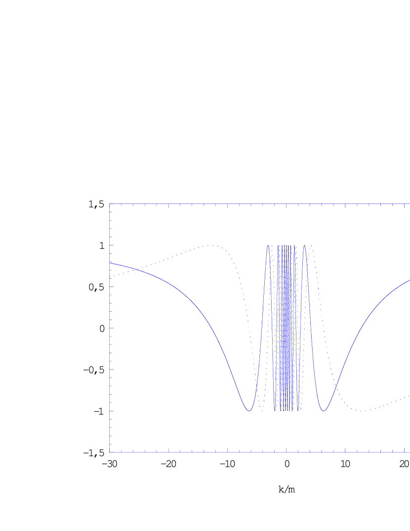
Figure 1: Real (solid) and imaginary (dots) parts of the solution, equation (23) for very weak differential rotation ($\alpha/2Am=20$). The finite imaginary part at $k\rightarrow/\infty$ is responsible for the singular behavior of the wave as $t\rightarrow\infty$.

The exponent in equation (24) varies rapidly when $k\sim m$. The method of stationary phase tells us that at a given radius $s$ the main contribution to the integral in equation (24) comes from the value of $k$ such that the exponent is stationary:

$$s+\frac{\alpha}{2A(k^{2}+m^{2})}=0$$ (25)

Using equation (9) we see that this gives a local wavenumber $k(s)$ such that it verifies the dispersion relation of Rossby waves, Doppler-shifted by the equilibrium rotation:

$$\omega-m\Omega(s)=\frac{m\alpha}{k^{2}+m^{2}}$$ (26)

with $\omega=m\Omega_{0}$. The wave propagates between $s=0$ (corotation, at large $k$) and a turning point ($k=0$) at:

$$s_{max}=-\frac{\alpha}{2Am^{2}}$$

Let us now consider the solution with

$$F=\delta(k-2Amt):$$

the $\delta$ function has the effect that the full solution $R(k,t)$ explores the separated one, equation(23), while $k$ varies from tightly wound leading ($k\rightarrow-\infty$) to tightly wound trailing ($k\rightarrow\infty$) because of the shear. The inverse Fourier transform gives:

$$R(s,t) = R_{0}\int_{-\infty}^{\infty}dke^{iks}\delta(k-2Amt)$$ (27)

$$\hskip 85.35826pt\exp\left(i\frac{\alpha}{2Am}\arctan\frac{k}{m}\right)$$

$$= R_{0}\exp\left[i\left(ks+\frac{\alpha}{2Am}\arctan\frac{k}{m}\right)\right]$$

where now $k=2Amt$. Again in the limit where differential rotation is weak, $A\ll\alpha$, the stationary phase tells us that at a given $s$ the perturbation is strong only when $k$ has the value given in equation (25), and at the corresponding time: we now have a description of a travelling Rossby wave, propagating from tightly leading ($k$ large and negative) at corotation at $t=-\infty$, to the turning point (at $t=0$) and back to corotation as tightly trailing ($k$ large and positive).

A qualitatively new and important result is obtained by considering the evolution of the wave at corotation: as $k$ varies the arctangent in equation (27) varies from $-\pi/2$ to $\pi/2$, so that the exponent varies between $\pm{\pi\alpha}/{4Am}$.

This means that at corotation the Rossby wave oscillates only

$$n_{oscillations}=\frac{\alpha}{4Am}$$ (28)

times before it gets sheared away by differential rotation. It always evolves, as $t\rightarrow\infty$, to a singular vortex (a jump in $v_{\vartheta}$ at $s=0$). This final evolution will occur even for arbitrarily weak differential rotation.

At $s\neq 0$ the solution still oscillates with time because of the $ks$ term in the exponent: this is only due to the fact that a feature which is stationary at $s=0$ is seen Doppler-shifted by differential rotation by an observer at a different radius. These results are still valid (since the solution, equation (23) is exact) when differential rotation is not weak, as in a keplerian disk, but their WKB interpretation in terms of propagating waves becomes blurred.

At this stage we have thus described, in an equivalent (by the method of stationary phase) to a WKB model, the propagation of a single Rossby wave in a disk with differential rotation.

In the normal mode solution ($F=Cte$), at $s=0$, the initial and final values of the integrand in equation (24) are different, also giving by inverse Fourier transform a singularity at corotation. In the standing pattern obtained with this choice of $F$, the Rossby wave becomes a stationary vortex.

In general the envelope function $F$ is given by the initial conditions, so that if they are regular initially (e.g. describing a localized wave packet) the Fourier transform will be well-behaved at infinity. The evolution will nevertheless lead to the same conclusion.

In the more general case where $A$ is not small, this evolution will be very rapid: in a keplerian disk ($A=\alpha$) the wave will describe only a fraction $1/4m$ of a cycle before it degenerates! This is the reason why Rossby waves cannot be seen in disks with a realistic vorticity gradient. It is also the reason why the corotation resonance is more efficient at low $m$, so that the CSS can be considered as a convenient approximation for $m\gg 1$.

4 Evolution of vortices

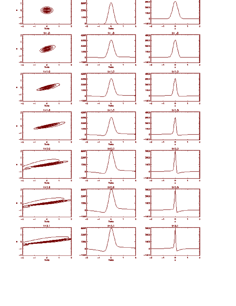
Figure 2: Evolution of a vortex in a differentially rotating disk. Contour plots, as well as cross sections at $\vartheta=0$ and $s=0$, are shown as time varies from $0$ to $\pi$, i.e. during a half rotation period.

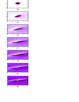
Figure 3: Same as figure 2, with color-coded contours showing more details.

Recent numerical studies (Bracco et al., 1998; Godon and Livio, 1999, 2000; Davis et al., 2000) have addressed the fate of vortices in protoplanetary disks. This was prompted by the work of Barge and Sommeria (1995), who had shown that a vortex would favor the formation of planets, by capture and coagulation of dust particles. These studies show that, as expected, vortices are rapidly sheared apart by differential rotation unless they are strong enough that non-linear effects allow them to survive for a significant time. This is obtained by Godon and Livio (1999, 2000) as embedded cyclonic and anticyclonic vortices. Davis et al. obtain longer lived anticyclonic vortices. The difference probably lies in the initial conditions given. In both cases this requires such strong amplitudes (locally reversing the rotation velocity gradient in the work of Davis et al.) that the mechanism which could create such vortices (supersonic if they are larger than the disk thickness) remains mysterious.

Here we will give a simple description of the linearized evolution of a vortex. We start from an initial gaussian vorticity perturbation, whose Fourier transform is:

$$R^{0}(m,k)=e^{-(m^{2}/m_{0}^{2}+k^{2}/k_{0}^{2})}$$ (29)

with $m_{0}=k_{0}=7$ for the numerical solution displayed. Using the previous results, we find that the envelope function for each Fourier component is given by:

$$F_{m}(k)=R^{0}(m,k)\exp\left[-i\frac{\alpha}{2Am}\arctan\frac{k}{m}\right]$$ (30)

giving the time evolution of the vorticity (after a convenient change of variables, $k\rightarrow k+2Amt$, in the inverse transform):

$$R (s,\vartheta,t)=\sum_{m}e^{im(\vartheta+2Ats)}e^{-m^{2}/m_{0}^{2}}\int_{-\infty}^{+\infty}dke^{iks}e^{-k^{2}/k_{0}^{2}}$$ (31)

$$\ \exp\left({i\frac{\alpha}{2Am}\left[\arctan(\frac{k}{m}+2At)-\arctan(\frac{k}{m})\right]}\right)$$

which is easily computed (as it would be with any other choice of initial condition). The result is displayed in figures 2 and 3. It shows that, as expected, the vortex is rapidly sheared away by differential rotation, reducing to the vorticity sheets described by Davis et al. (2000). It applies (since this is linear theory) to positive or negative vorticity, ı.e. cyclonic or anticyclonic vortices, and corresponds to the evolution observed for all but the highest amplitude vortices studied in non-linear simulations. An obvious extension would be to include compressibility, i.e. return to the full third-order system of equations, and solve it numerically for the equivalent of the incompressible solution, equation (23).

5 Discussion

We have derived, from the equations describing a differentially rotating disk, a model (which we call the Rossby Shearing Sheet) which retains the intrinsic simplicity of the conventional Shearing Sheet (obtained with only differential rotation) or the $\beta$-plane approximation (obtained with only differential vorticity) while including both gradients. The model results in a third order system of ordinary differential equations, rather than second order as in the CSS or first order in the $\beta$-plane approximation. This means that, besides inward- and outward-propagating spiral density waves, it incorporates the physics of Rossby waves.

In a first application, we have used incompressibility to separate the propagation of Rossby waves; we have shown that, for any ratio $A/\alpha$ between differential rotation and differential vorticity, the wave always collapses after a finite time to a singular vortex (a jump in $v_{\vartheta}$ at its corotation radius). In a realistic disk, this evolution is so fast that it occurs before the wave has completed even one cycle of oscillation. In a planetary atmosphere, on the other hand, zonal circulation should result in a lower ratio $A/\alpha$ and a slower evolution of the wave, but still in its collapse to a singular vortex in a finite time.

We have also described the linear evolution of a vortex in a keplerian disk, showing (as observed in non-linear simulations) that it reduces to a thin vorticity sheet in a very short time. This confirms that, unless a very strong non-linear mechanism can be found to maintain a vortex against shear, there is little hope of forming planets in this manner.

Lifting the constraint of incompressibility, we find that the density waves and Rossby waves are no more independent: this means that they are coupled by differential rotation in the disk. Waves loose their identity (the solutions are no more separated), so that a density wave generates a Rossby wave, and reciprocally. This process, in which energy and angular momentum are exchanged leading to growth or damping of the waves, is known as corotation resonance (but was not analyzed in terms of coupling to the Rossby wave) in studies of the spiral instability, with or without the long-range action of self-gravity or magnetic stresses. In the latter case it has recently been found to make an important contribution, leading to what we have called an Accretion-Ejection instability. In recent works, Lovelace et al. (1999) and Li et al. (2000) have also found an instability of unmagnetized disks, when the specific vorticity profile has an extremum.

Actually our result already allows us to give a physical interpretation for the sign of the corotation resonance: we found that a Rossby wave can propagate only between corotation and a radius $s_{max}=-\alpha/2Am^{2}$, ı.e. inside corotation if $\alpha$ and $A$ have the same sign: since a wave propagating inside corotation has negative energy and angular momentum (see e.g. Collett and Lynden-Bell, 1987) we conclude that a spiral wave propagating inside corotation will be damped by exciting a Rossby wave. On the other hand we have mentioned that in fact the relevant gradient for Rossby waves is that of specific vorticity, $W/\Sigma$, or of $W\Sigma/B^{2}$ in a magnetized disk. Thus if these gradients change sign, they will also change the sign of $s_{max}$ so that the Rossby wave will now propagate beyond corotation, and will have a positive energy. This means that exciting it will amplify a spiral wave.

Future work will be dedicated to using this model for a deeper analysis of the coupling between density and Rossby waves, in accretion disks and in planetary atmospheres.

References

- (1) Barge, P. & Sommeria, J., 1995, A&A 295, L1
- (2) Binney, J. and Tremaine, S., 1987, Galactic Dynamics, Princeton University Press
- (3) Bracco, A., Chavanis, P.H. &Provenzale, A., 1998, Phys. Fluids 11, 2280
- (4) Collett, J.L. & Lynden-Bell, D., 1987, MNRAS 224, 489
- (5) Davis, S.S., Sheehan, D.P., and Cuzzi, J.N., 2000, ApJ 545, 494
- (6) Godon, P. & Livio, M., 1999, ApJ 523, 350
- (7) Godon, P. & Livio, M., 2000, ApJ 537, 396
- (8) Li, H. Finn, J. M. Lovelace, R. V. E. and Colgate, S. A., 2000, ApJ 533, 1023L
- (9) Lin,C.C., and Thurstans , R.P.: 1984, in Proc. of a course on Plasma Astrophysics, Varenna, Italy, ESA S.P. 207 (Noordwijk, Holland), 121
- (10) Lovelace, R. V. E., Li, H., Colgate, S. A. and Nelson, A. F., 1999, ApJ 513, 805L
- (11) Narayan, R., Goldreich, P. and Goodman, J., 1987, MNRAS 228, 1
- (12) Pannatoni, R.F., 1983, Geophys. Ap. Fluid Dyn. 24, 165
- (13) Papaloizou, J.C.B. and Pringle, J.E., 1984, MNRAS 208, 721
- (14) Papaloizou, J.C.B. and Pringle, J.E., 1985, MNRAS 213, 799
- (15) Papaloizou, J.C.B. and Lin, D.N.C., 1989, ApJ. 344, 645
- (16) Tagger, M., Henriksen, R.N., Sygnet, J.F. and Pellat, R., 1990, ApJ 353, 654
- (17) Tagger, M., and Pellat, R., 1999, A& A 349, 1003