Automated Galaxy Morphology: A Fourier Approach

Abstract

We use automated surface photometry and pattern classification techniques to morphologically classify galaxies. The two-dimensional light distribution of a galaxy is reconstructed using Fourier series fits to azimuthal profiles computed in concentric elliptical annuli centered on the galaxy. Both the phase and amplitude of each Fourier component have been studied as a function of radial bin number for a large collection of galaxy images using principal component analysis. We find that up to 90% of the variance in many of these Fourier profiles may be characterized in as few as 3 principal components and their use substantially reduces the dimensionality of the classification problem. We use supervised learning methods in the form of artificial neural networks to train galaxy classifiers that detect morphological bars at the 85-90% confidence level and can identify the Hubble type with a $1\sigma$ scatter of 1.5 steps on the 16-step stage axis of the revised Hubble system. Finally, we systematically characterize the adverse effects of decreasing resolution and $S/N$ on the quality of morphological information predicted by these classifiers.

Date of this version:

Subject headings: galaxies: automated morphological classification

1 INTRODUCTION

One of the earliest galaxy classification schemes, discussed by Hubble (1926), was based on the visual appearance of two-dimensional images. This and other early schemes, based largely on photographic images in roughly the $B$ bandpass, used global image properties such as the visually perceived bulge-to-disk ratio and the degree of azimuthal surface brightness symmetry as major classification criteria. Even these early systems discussed the presence of spiral structure and the overall characteristics of the spiral arms: grand design of high or low pitch angle verses patchy or multiple arms (later termed flocculent spirals). The early Hubble system delineated spirals into a parallel sequence of barred and unbarred disk galaxies in a two-dimensional system. A refinement of this approach by de Vaucouleurs (1959), established a three-dimensional classification volume with the major axis being the Hubble stage (E,S,I) and the two other axes representing family (barred or unbarred) and variety (ringed or non-ringed). The revised Hubble system (hereafter referred to as the RHS) was designed to describe a continuum of morphological properties. Early workers in the field strove to systematize the degree of visual structures we see in galaxies (bulge/disk ratio, spiral arms, bars, rings) in an effort to understand the physical processes that formed these different galaxies.

A useful classification system must relate members of different classes to well understood general properties of the objects being systematically classified. It has long been known (de Vaucouleurs 1977, Buta et al. 1994, and Roberts and Haynes 1994) that the stage axis of the Hubble sequence produces smooth, strong correlations with well known global properties: color, surface brightness, maximum rotational velocity, and gas content. These measured quantities are linked directly to very important physical properties: stellar population fraction, the surface density of stars, total mass of the system, and the rate of conversion of gas to stars. As discussed by Odewahn and Aldering (1995), such correlations may be smooth and significant in a mean sense, however the degree of accidental scatter in these relations is quite large. In most cases this scatter is much larger than that introduced by measurement error and is clearly cosmic in origin. The family and variety estimates of the RHS produce much less significant correlations with such properties. Buta and Combes (1995), in an excellent review of these morphological features, make clear that family and variety convey information about the specific dynamical properties of disk systems: the degree of differential rotation, the presence of certain families of resonant orbits among the stellar component of the disk, and the response of the viscous disk components (the gas) to the global and local properties of the galaxy potential well.

Galaxy classification systems are generally built on the visual appearance in an image, and hence data sets based on these systems can be gathered from imaging surveys alone. The mean correlations described above are then used to draw inferences about important physical processes describing galaxies via these catalogs. In other words, morphological classification provided a ”cheap” and direct means of acquiring large statistical samples describing galaxies. In some respects, the qualitative nature of this classification approach, and the dearth of recognized experts who classified in some established system gave the approach a less than deserved poor reputation. However, even recent comparisons among the estimates of experienced human classifiers (Naim et al. 1995) show a reliable level of repeatability is achieved. With an expansive increase in the quantity and quality of galaxy images in the last decade data via HST and a host of ground-base imaging surveys, interest has returned to the field of morphological classification (Driver et al. 1995a,b; Glazebrook et al. 1995; Abraham et al. 1996; Odewahn et al. 1996). Many workers have developed automated image analysis systems that provide quantitative estimates of galaxy types (Okamura et al. 1984, Whitmore 1984, Spiekermann 1992, Storrie-Lombardi et al. 1992, Abraham et al. 1994, Odewahn 1995, Han 1995, Odewahn et al. 1997). In one the most physically meaningful approaches, Rix and Zaritsky (1995) showed in a small sample of spiral galaxies that kinematic distortions in the global velocity field of a galaxy can be linked to global asymmetry measurements in the light distribution. A discussion of novel feature spaces for identifying peculiar galaxies is presented by Naim et al. (1997). All of these studies have produced a wealth of information about the systematic properties of galaxies, particularly in the area of comparing the low and high redshift Universe (Abraham et al. 1996, Odewahn et al. 1996). However, it must be conceded that none of these classification systems are truly morphological in nature. In general, each method uses one or more two-dimensional parameter spaces based on global image properties and produces a type estimate via mean correlations like those discussed above using some multivariate pattern classification approach (e. g. linear parameter space divisions, principal component analysis, decision tree, artificial neural network).

In this paper we describe a truly morphological approach to galaxy classification based on the Fourier reconstruction of galaxy images and the subsequent pattern analysis based on the amplitude and phase angle of the Fourier components used. This method can quantitatively detect the presence of spiral arms and bars. In addition, it provides a systematic means of describing the degree of large-scale global asymmetry in a galaxy, a property known to correlate loosely with Hubble stage, but one which is also strongly linked to important physical events such as merging and tidal interaction.

In Section 2 we describe our machine-automated classification method. In Section 3 we compare independent sets of visual estimates of morphological types in the RHS that establish a well understood set of training/testing cases. These date are comprised of a local sample from ground-based imaging and a distant sample collected from the HST archive. In Section 4 we demonstrate a practical application using these data to train and assess the performance of several Fourier-based galaxy classifiers. We discuss the role of systematic and accidental errors in its use caused by varying image resolution and $S/N$ . In Section 5 we summarize the results and lay the groundwork for future morphological studies of distant galaxy populations.

2 CLASSIFICATION METHODOLOGY

The two-dimensional luminosity distribution observed in most galaxies most often displays a high degree of azimuthal symmetry. This justifies the use of one-dimensional radial surface brightness profiles in describing the radial stellar surface density distribution. Such profiles are then decomposed into constituent photometric components (de Vaucouleurs 1958, de Vaucouleurs and Simien 1986, Kent 1986, de Jong and van der Kruit 1994). This profile is extracted from the galaxy image in many ways, but most often by computing mean flux density in elliptical annuli having the shape and orientation of the faint surface brightness, outer isophotes. Parameterizing this profile, c. g. with a concentration index, will produce a measurement that correlates well with bulge-to-disk ratio and hence with Hubble type. Local departures from this overall radial symmetry in the form of high spatial frequency components (arms, bars, rings) form the basis for additional criteria to visual galaxy classification systems like the RHS.

A method which quantitatively describes departures from azimuthal symmetry in galaxy images would seem to be a rich starting place for developing a machine automated classification system, either of the supervised learning variety (Odewahn et al. 1992, Weir et al. 1995) or the unsupervised variety (Mahonen et al. 1995). Towards this end, we have adapted a moments-based image analysis technique (Odewahn 1989) to fit Fourier components to fixed-grid azimuthal profiles in elliptical annuli to reconstruct galaxy images. One may think of this step as an optimized data compression technique for reducing the dimensionality of our ultimate pattern classification problem: the recognition and characterization of morphological features in galaxies.

The technique of Fourier decomposition presented here is used to quantify the two dimensional luminosity distributions of galaxies. Similar approaches have been used to study the shapes of isophotes in elliptical galaxies by Bender and Mollenhoff (1987), and applications to the luminosity distribution are described by Lauer (1985), Buta (1987), and Ohta (1990). With this methodology, we can quantify the amplitude and phase of the bar and spiral arm components in a galaxy image. This technique is very useful for modeling the bar luminosity distribution for systems in which a simple elliptical bar model was not sufficient, as was first demonstrated by Elmegreen and Elmegreen (1985) in describing the bar luminosity distributions exhibited by galaxies over a range of Hubble types.

2.1 Pattern Classification Using Artificial Neural Networks

Artificial neural networks (ANN’s) are systems of weight vectors, whose component values are established through various machine learning algorithms. These systems receive information in the form of a vector (the input pattern) and produce as output a numerical pattern encoding a classification. They were designed to simulate groups of biological neurons and their interconnections and to mimic the ability of such systems to learn and generalize. Discussion of the development and practical application of neural networks is well presented in the literature (see McClellan and Rumelhardt 1988). In astronomical applications, this technique has been applied with considerable success to the problem of star-galaxy separation by Odewahn et al. (1992). A neural network classifier was developed Storrie-Lombardi et al. (1992) to assign galaxy types on the basis of the photometric parameters supplied by the ESO-LV catalog of Lauberts and Valentijn (1989). Applications of this method to large surveys of galaxies using photographic Schmidt plate material are discussed in Odewahn (1995) and Naim et al. (1995). More recent discussions of star-galaxy separation using ANN’s are presented by Andreon et al. (2000), Mahonen & Frantti (2000), and and Philip et al. (2000). An extremely thorough discussion of galaxy classification with ANN methods is given by Bazell (2000).

The neural network literature quoted above contains a wealth of information on the theoretical development of neural networks and the various methods used to establish the network weight values. We summarize here only the practical aspects of the ANN operation and the basic equations for applying a feed-forward network. The input information, in our case the principal components formed from the Fourier profiles discussed in Section 3.2, is presented to the network through a set of input nodes, referred to as the input layer. Each input node is “connected” via an information pathway to nodes in a second layer referred to as the first hidden layer. In a repeating fashion, one may construct a network using any number of such hidden layers. For the backpropagation networks discussed here, we have used ANN’s with two hidden layers. The final layer of node positions, referred to as the output layer, will contain the numerical output of the network encoding the classification. This system of nodes and interconnections is analogous to the system of neurons and synapses of the brain. Information is conveyed along each connection, processed at each node site, and passed along to nodes further “upstream” in the network. This is referred to as a feed-forward network. The information processing at each node site is performed by combining all input numerical information from upstream nodes, $a_{pj}$, in a weighted average of the form:

$$\beta_{i}=\sum_{j}w_{ij}a_{pj}+b_{i}$$ (1)

The $j$ subscript refers to a summation of all nodes in the previous layer of nodes and the $i$ subscript refers to the node position in the present layer, i.e. the node for which we are computing an output. Each time the ANN produces an output pattern, it has done so by processing information from the input layer. This input information is referred to as the input pattern, and we use the $p$ subscript to indicate input pattern. Hence, if there are 5 nodes in the previous layer ($j$), each node ($i$) in the current layer will contain 5 weight values ($w_{ij}$) and a constant term, $b_{i}$, which is referred to as the bias. The final nodal output is computed via the activation function, which in the case of this work is a sigmoidal function of the form:

$$a_{pi}=\frac{1}{1+\exp^{-\beta_{i}}}$$ (2)

Hence, the information passed from node $i$ in the current layer of consideration, when the network was presented with input pattern $p$, is denoted as $a_{pi}$. This numerical value is subsequently passed to the forward layer along the connection lines for further network processing. The activation values computed in the output layer form the numerical output of the ANN and serve to encode the classification for input pattern, $p$.

In order to solve for the weight and bias values of equation 1 for all nodes, one requires a set of input patterns for which the correct classification is known. This set of examples is used in an iterative fashion to establish weight values using a gradient descent algorithm known as backpropagation. In brief, backpropagation training is performed by initially assigning random values to the $w_{ij}$ and $b_{i}$ terms in all nodes. Each time a training pattern is presented to the ANN, the activation for each node, $a_{pi}$, is computed. After the output layer is computed, we go backwards through the network and compute an error term which measures of the change in the network output produced by an incremental change in the node weight values. Based on these error terms, all network weights are updated and the process continues for each set of training patterns. As discussed in the next section, precautions must be taken in this process to avoid problems from over-training (i. e. simply memorizing the input pattern set as opposed to generalizing the problem).

The goal of the present work is to develop a system that automatically detects the presence of specific types of morphological structures in galaxy images. This is clearly a more complex problem compared to the use of a few global photometric parameters to predict types, and so we desired to use an additional method of neural network classification to confirm the results of our classical backpropagation approach. Philip et al. (2000) develop a neural network based on Bayes’ principal that assumes the clustering of attribute values (the input parameters). The method considers the error produced by each training pattern presented to the network, and weights are updated on the basis of the Bayesian probability associated with each attribute for a given training pattern. In this approach, the probability density of identical attribute values flattens out while attributes showing large differences from the mean get boosted in importance. This is referred to as a difference boosting neural network (DBNN). We have applied this new approach as a check on our backpropagation network results, however this method has the added advantage that it trains to convergence in a much faster time than is required by classical backpropagation methods.

2.2 Initial Image Reconstruction

In this paper we develop a technique that is a pre-processing step for producing input to a supervised classifier in the form of an artificial neural network (Odewahn 1997). In this approach, the radial surface brightness profile of a galaxy is computed in elliptical annuli centered on the galaxy center. The rational here, valid in most cases, is that we are isolating the disk component of the galaxy and hence establishing a way of defining the equatorial plane of the system. The position, shape and orientation of these annuli are determined using classical isophotal ellipse fitting techniques. Within each annulus, we compute the run of flux density with position angle, $\theta$, in the equatorial plane of the galaxy, to form the azimuthal surface brightness profile. To describe each azimuthal profile, and reduce the dimensionality of our classification problem, each azimuthal profile is modeled by the following Fourier series:

$$I_{o}(r,\theta)=I_{\circ}+\Sigma I_{mc}(r)\cos m\theta+\Sigma I_{ms}(r)\sin m\theta$$ (3)

For computational efficiency, the Fourier terms are computed for each azimuthal profile using the following moment relations :

$$I_{o}(r)=<I(r,\theta)>$$ (4)

$$I_{mc}(r)=2<I(r,\theta)\cos m\theta>$$ (5)

$$I_{ms}(r)=2<I(r,\theta)\sin m\theta>$$ (6)

where $\theta$ is the angle (in the equatorial plane of the galaxy) with respect to the photometric major axis, and m is an integer. Hence, if we assume galaxy disks to be thin and suffer no internal extinction, this approach crudely removes inclination effects and allows us to compare galaxy images independent of orientation. The Fourier series in this paper were computed up to m=5. Fourier amplitudes, describing the relative amplitude of each component are computed using the following expression :

$$A_{m}(r)=\sqrt{I_{mc}(r)^{2}+I_{ms}(r)^{2}}/I_{o}(r)$$ (7)

Finally, a phase angle describing the angular position of the peak signal contributed by each component can be computed. We compute the phase angle of the $m\theta$ component as:

$$\theta_{\circ}=(1/m)\tan^{-1}(I_{ms}/I_{mc})$$ (8)

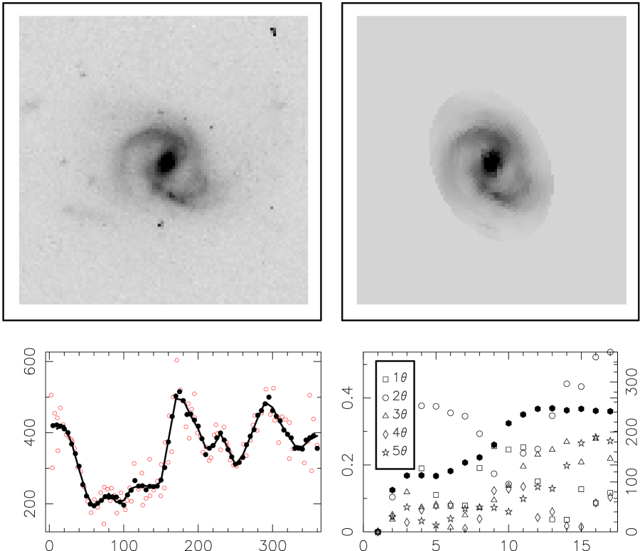
Figure 1: The Fourier image-modeling method described in the text applied to a galaxy observed with HST in the B-Band Parallel Survey (BBPS, Cohen et al. 2001). The original $I$ image is shown in the upper-left panel, and the Fourier model image is shown in the upper-right. In the lower-left panel we plot the azimuthal profile for the annulus over-plotted in the galaxy image. Open circles are individual pixel values, solid points represent the smooth points, and the solid line represents the Fourier series fitted to this profile. In the lower-right panel we plot the five Fourier amplitudes as a function of radial annulus number using open symbols (left numeric scale). Finally, the solid points represent the phase angle, measured in degrees in the equatorial plane, of the 2$\theta$ component (right numeric scale).

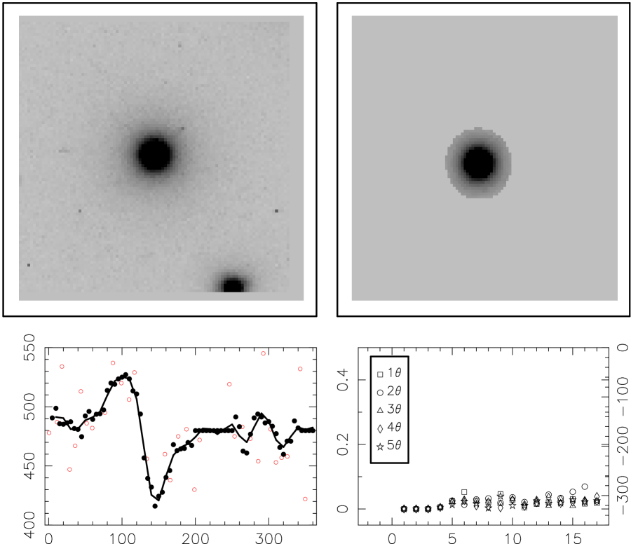
Figure 2: The same style of figure as in Figure 1, except we now measure an early-type galaxy from the BBP. In this case, there is little high spatial frequency image structure and only very small departures from radial symmetry. Hence, the Fourier amplitudes, plotted to the same scale as in Figure 1, are very small. Additionally, no phase angles are plotted since the $2\theta$ Fourier amplitudes were below the $S/N$ limit imposed for computing these angles.

A practical application of this method to a barred spiral galaxy imaged with HST is shown in Figure 1. Another example for an elliptical galaxy image which contains no high spatial frequency image structure is shown in Figure 2. Through experimentation with both HST- and ground-based images, we have determined that using 17 elliptical annuli and up to $m=5$ in Equation 3 consistently reproduces the basic morphological features of most galaxy images. A considerable amount of experimentation went into determining how one should establish the radial bin intervals in this procedure. A series of tests were made using unequal linear bins that overlapped and logarithmic binning interval. We experimented with normalizing the bin radius by the effective radius, $r_{e}$, so that all galaxies could be compared on more uniform spatial scale. This approach proved problematic since it produced profile scales that were highly compressed for early-type systems, a highly expanded in late-type systems. In such cases, the inner regions if the late-type galaxies, where much of the important morphological structure is present, was under-resolved. Additionally, we found that measurement of the effective radius of galaxies in low resolution, low $S/N$ HST images can be systematically low, and using $r_{e}$ in this manner will introduce a substantial bias when comparing local and distant samples. In the end, we found that using equal size radial bins extending to an outer, low surface brightness optical isophote produce the most robust results for comparing morphological properties among galaxy images.

It should be noted that one can justify the use of higher order Fourier components for cases of high resolution galaxy images. In experiments with some of the deep Palomar 60^′′ images described in Section 3, we found that the bars of many galaxies have a strong contrast relative to the disk, and high spatial frequency components (up to $12\theta$) are required to reconstruct such a sharp feature. Incorporating so many spatial frequencies in a general image classifier is impractical, but one might hope to use some type of information about high frequency structure: if the inclusion of such components in the model significantly improves the model fit, then this is important information. Perhaps a good number of barred galaxies can be identified if we simply search for images that require high order Fourier components in the inner annuli to build a good fit model.

2.3 Dimensionality Reduction using Radial Trends

The Fourier-reconstructed images described above are comprised of radially-dependent sets of Fourier amplitudes and phase angles. Using 17 annuli, 6 Fourier amplitudes (including the $m=0$ term) and the corresponding phase angles to parameterize each image, we thus describe each galaxy with a 221 element classification vector. Some human classifiers have insisted that at least 10,000 resolution elements are required in a galaxy image that is to be morphologically classified (de Vaucouleurs, private communication). More liberally, we might consider that one should have at least a $50\times 50$ image of a galaxy, or 2500 pixels, to convey morphological information. Hence, using the Fourier description of a galaxy reduces the number of parameters describing the image information content by a factor of more than ten compared to that used by a human classifier. An input classification vector with over 100 elements is rather large for most pattern classifiers trained in the presence of noise. To distill our image parameterization further, we have chosen to characterize the radial properties of each Fourier component. In other words, just as we often describe the radial surface brightness profile of a galaxy using several model parameters, so too can we describe the radial trends in each set of amplitude and phase estimates computed with equations  7 and  8.

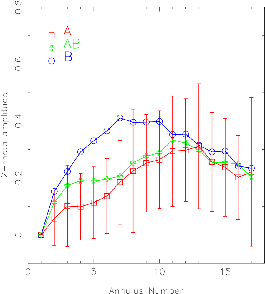
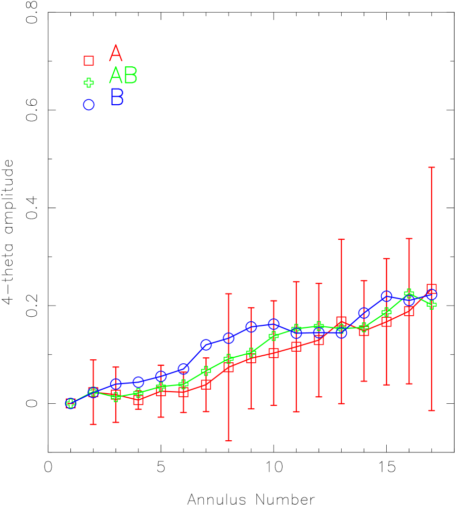
Figure 3: Mean profiles of the $2\theta$ (left) and $4\theta$ (right) amplitudes computed for three sets of galaxies divided by family class. We used 71 A, 73 AB, and 61 B galaxies. The mean barred (B) galaxy trends are well separated from unbarred (A) galaxies for annuli numbers (on the x-axis) in the range 3 to 12. We plot the $1\sigma$ error bars for the mean A points only. It is significant that in both the $2\theta$ and $4\theta$ cases the mean AB profiles lie between the A and B curves indicating that these galaxies do indeed possess only weakly detected bar structures.

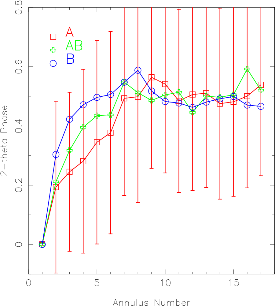
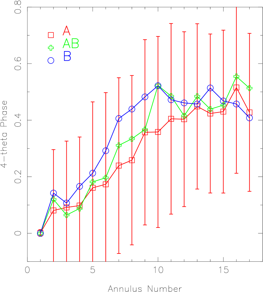
Figure 4: Mean profiles of the $2\theta$ (left) and $4\theta$ (right) phase computed for the same samples used in Figure 3. Although amplitude information clearly provides a more powerful means of detecting the presence of a bar, phase information is needed to differentiate between a purely linear structure like a bar and a simple two-armed spiral pattern.

The mean radial trends in both the amplitude and phase of the coefficients in equations  7 and  8 are shown in Figures  3 and  4 for three types of galaxies. In these figures the mean phase or amplitude of a given Fourier component is plotted on the y-axis as a function of elliptical annulus number on the x-axis. We divided a sample of 196 galaxies from Section 3 into three family categories: A (unbarred system), AB (transitional systems), and B (barred systems) and computed the mean radial profiles for the amplitude and phase coefficients of the $2\theta$ and $4\theta$ coefficients. As noted by Elmegreen and Elmegreen (1985) and Ohta (1990), these are the dominant terms needed to reproduce the light distributions of most barred galaxies. In Figure 3 we see a clear trend among the $2\theta$ and $4\theta$ amplitudes: barred systems have significant power in the inner rings, AB systems have systematically lower power, and A galaxies have the lowest amount of $2\theta$ and $4\theta$ power in even the inner elliptical annuli. These mean profiles were computed with 71 A, 73 AB and 61 B galaxies taken from the analysis of Section 4. The 1-$\sigma$ error of each point in the A-system profiles are shown in Figures  3 and  4, and it is clear that a single point from the profile of one galaxy will have little discriminatory power in distinguishing bar class. However, if we combine the information of the points from annuli with ring numbers between 3 and 12, then we can expect to derive a robust estimate of whether a bar is present in the inner regions of a galaxy image. In this region of the reconstructed images, the mean Fourier profiles clearly delineate the presence of a bar. In Figure 4 we plot the corresponding mean profiles for the $2\theta$ and $4\theta$ phase angles. Although these profiles are less sensitive to bar presence, the phase terms will be important in distinguishing barred galaxies from purely spiral systems. In the case of a barred galaxy, the $2\theta$ and $4\theta$ phase angles remain fixed with ring number (radius), whereas with a two-armed spiral pattern we expect to see a systematic variation of $2\theta$ and $4\theta$ phase angles with radius since the flux density peaks are changing their position angle smoothly as we progress outward in the radial annuli. As can be seen in Figure 4 we still observe a gradual progression in the trends of these phase angle profiles for the A, AB, and B galaxy sets. To summarize, the radial $2\theta$ and $4\theta$ amplitude and phase angle profiles of a galaxy carry important information about the nature of the 2-D structure present in a galaxy image, and specifically allow us to robustly quantify the presence of a linear bar structure.

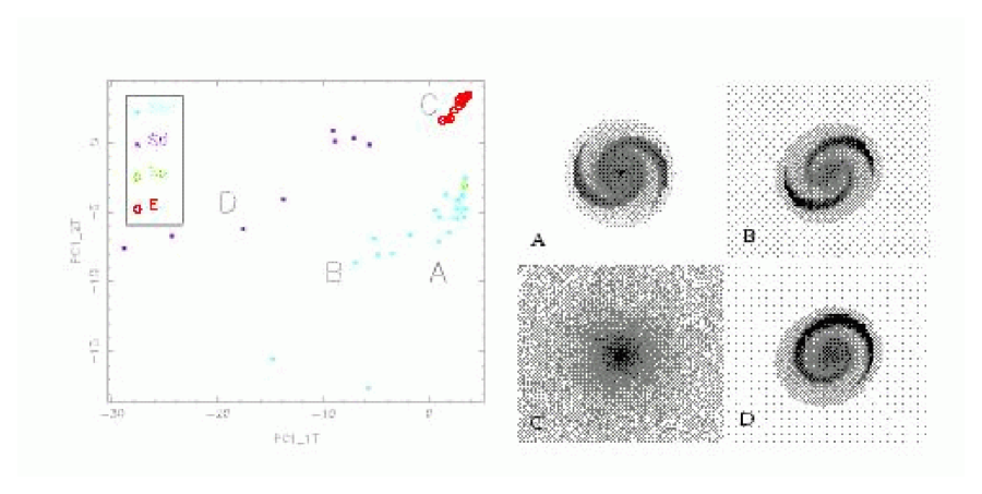
Figure 5: (a) [Left] A parameter space formed from the first principal component of the 1$\theta$ Fourier amplitude profile, PC_1T, and the first principal component of the 2$\theta$ Fourier amplitude profile, PC_2T. The large letter labels correspond to the images in the right panel. (b) [Right] Sample model images produced by LMORPHO that were used to compute the parameter space in the left-hand panel. Objects in the top row (A,B) are idealized mid-type spirals (with B inclined assuming an optically thin disk model), object C (lower left) is a typical elliptical model, and object D (lower right) is the one-armed spiral morphology often seen in compact groups (see compact group 16 in the catalog of Hickson 1993). We have used model galaxy images in this figure to clearly demonstrate the power of the method, but tests with real galaxy images have been found similarly effective.

Following the innovative work of Han (1995), we performed a principal component analysis (PCA) of each set of Fourier profiles for our collections of galaxies that had reliable stage and family classifications. For most Fourier coefficients it was determined that 85% to 90% of the profile variance could be described with only 2 or 3 principal components. Hence, using the eigenvectors determined from this analysis, we can characterize the Fourier profile of a random galaxy using only 2 or 3 parameters. Should we use the amplitude and phase of only the $2\theta$ and $4\theta$ components to characterize a galaxy, then we can parameterize the light distribution using 4 coefficients $\times$ 2 principal components $=$ 8 parameters. Such an image vector constitutes a very reasonable size for training a supervised classifier with the 100-200 patterns (galaxies) available in this work. In Figures  3 and  4 we have divided the galaxies by family class, but these Fourier-based principal components may be used to identify stage-related image traits also. In Figure 5 we demonstrate our principal component method by showing PCA-based image parameter spaces that are symbol coded by stage and family class.

3 TRAINING AND TESTING SAMPLES

The development of a pattern classifier based on supervised learning, i. e. a classifier that works in a predefined system, requires a data sample consisting of the input classification information (the image parameters) and the corresponding target patterns (the galaxy types). This sample is referred to as the training set, and a portion of it is held back from the actual supervised learning process (in our case backpropagation training) to be used as a test sample to make an unbiased judgement of classifier performance during and after training. As we discuss below, nearly all of the past morphology-based studies of high redshift galaxies have focused on the stage axis only. Since our aim is to develop morphological classifiers that estimate the family and variety of galaxies based on Fourier amplitude strengths and phases, we have visually reclassified a large number of high $S/N$ , well-resolved HST galaxy images in the RHS to establish a statistically significant testing sample. Although the present sample is based on 35 medium-deep and deep WFPC2 fields, the number of galaxy images from this sample that are suitable for such classification is only 146. Hence, for the present study we incorporated the local galaxy samples from ground-based CCD observations by de Jong and van der Kruit (1995), hereafter J95, and Frei et al. (1996), hereafter F96, adding 124 more galaxies to the sample. For both the local and distant HST samples we inter-compare our classification sets in order to objectively define a weighted mean training set whose systematic and accidental errors are well understood. From such a sample we may establish a fair ”ground-truth” sample of objects for use in training and testing pattern classifiers.

A large collection of visual Type estimates in several bandpasses from WFPC2 deep fields were discussed in Odewahn et al. (1996) and Driver et al. (1995b). Similar visual classification sets have been assembled since that time for the Hubble flanking fields (Odewahn et al. 1997) and the BBPS fields (Cohen et al. 2001). To begin our assessment of classifier errors, we have analyzed a large number of past visual stage estimates made in the F814W bandpass images. We inter-compared all of the stage estimates common to the 5 classifiers of Odewahn et al. (1996) and the DWG sample and derived linear transformations to convert all classifiers to a common system. The vast majority of classifications were from one classifier (1000 from Odewahn, hereafter referred to as SCO). It was decided that the Odewahn classes, which match well the RC3 mean Type system, would define the HST classification system. Following Odewahn and de Vaucouleurs (1993) we then use a residual analysis to determine the accidental scatter associated with each classifier, and hence a relative weight associated with each classification of an HST-observed galaxy. Finally, a catalog of 1306 galaxy types was assembled: 1000 with single Odewahn estimates with mean error of $\pm 2.2$ type steps and 306 weighted mean types (109 having 5 independent estimates) with mean error of $\pm 1.2$ type steps. The galaxies in this catalog have stage estimates from the the F814W images and objective errors estimated for each type. These data will hereafter be referred to as the HST1 set.

The purpose of our current work is to develop automated techniques that identify morphological structures, and with the exception of the bright BBP galaxy types estimates of SCO, the HST1 types are comprised only of estimates of the stage axis in the RHS (i. e. E, S0, Sa, …, Im). Such data sets are fine for the type classifiers discussed in Odewahn et al. (1996), however for more advanced classification experiments we desired a set of faint HST-observed galaxies with classifications in the RHS: stage, family and variety. To collect this set we extracted 4534 galaxy images in F814W from 39 different WFPC2 fields. The majority of these images were contributed by moderate depth WFPC2 parallel fields, but the deep 53W002 and HDF-N fields were also used. From this sample we established, purely through visual inspection, the group of 146 galaxy images having sufficient $S/N$ and resolution to allow good morphological classification. As a second sample, we binned 125 ground-based CCD images of F96 (in Gunn g) and J95 (in Johnson B) to a resolution similar to that of the HST images.

The manipulation of all galaxy images used in this work, whether for the purpose of human visual classification or for automated image analysis was performed with a variant of the MORPHO package discussed in Odewahn et al. (1997). A new version of this galaxy morphological classification software system called LMORPHO, which is optimized for use under the linux operating system, provides an image database manager that allows users to select galaxies for analysis based on morphological traits, photometric properties or many other meta-data properties (c. g. bandpass, image size, or pixel scale). Beyond the image database manager of LMORPHO, the system provides tools performing automated galaxy surface photometry, basic astronomical image processing, and a variety of multivariate statistical analysis and pattern classification tasks.

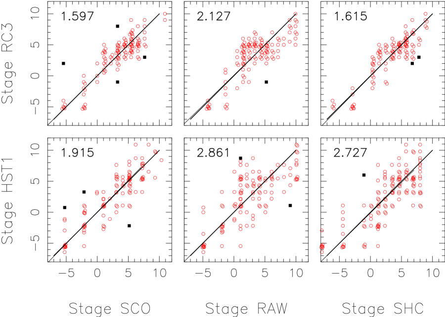
Figure 6: Correlations between the revised Hubble type stage estimates made by different classifiers. Small scale and zeropoint adjustments were made to each set in order to bring all catalogs onto the system defined by RC3 stage estimates. Using the method discussed in Odewahn and de Vaucouleurs (1993) we derived the accidental error associated with each classifier.

Our galaxy image libraries were independently inspected by three classifiers using an LMORPHO graphical galaxy classification tool. The three classifiers were SCO, Windhorst (hereafter RAW), and Cohen (hereafter SHC), and each visually estimated the stage, family, and variety for each of the 272 galaxy images in the adopted sample. For a variety of reasons (insufficient $S/N$ or resolution, high inclination, etc…) certain aspects of the classification (usually the family and variety) were uncertain and these were designated as unknown. Following the method used for the HST1 sample, we next inter-compared these type catalogs in order to establish the systematic and accidental errors associated with each set. The results of this are summarized in Table  1 and Figure 6. For the local galaxy samples, we compared each classifier to the weighted mean types in the RHS contained in the RC3 and discussed in Buta et al. (1994). For the distant sample we compared each classifier’s types with the weighted mean types of HST1. Although many of the HST1 types are indeed weighted means of several independent estimates, the majority are single estimates from SCO and hence we should regard the HST1 set as an independent (SCO-dominated) unit-weight catalog.

For both the local and distant galaxy samples, a preliminary linear regression analysis was performed to determine transformation relations for converting to the RC3 and HST1 systems respectively. An impartial regression analysis, using each catalog as the dependent variable, was used to determine the mean relationship between all possible catalog pairs. For each sub-sample (local and distant), small scale and zeropoint shifts were applied to the SCO, RAW and SHC stage estimates to bring all classifications onto a uniform system. It is informative to note that the size and sense of the scale corrections were uniform by classifier irrespective of local or distant sample: SCO and RAW systematically classified galaxies later at the 8% level, and SHC systematically classified galaxies earlier at the 6% level. These scale adjustments were statistically significant at the $2\sigma$ level. The zeropoint shifts, statistically significant at the $3\sigma$ level, were general less than one step on the 16-step stage axis of the RHS (with the exception of a $-2.2$ step correction for the distant RAW sample). In each case (local and distant) mean transformation equations were derived for the SCO, RAW, and SHC classification sets. Following these small, but statistically justified, transformations a second correlation analysis was performed to verify system uniformity and to compute the mean variance associated with each catalog comparison. This analysis is illustrated in the top panel of Figure 6 for the local sample and in the bottom panel for the distant (HST) sample. With all stage estimates transformed to a common mean system, we followed the methodology of Odewahn and de Vaucouleurs (1993) to compute the mean standard deviation of the $2\times 2$ residuals in each comparison (these values are plotted in each panel of Figure 6). These estimates were combined via a system of linear equations to calculate the standard deviation associated with each individual catalog. The results, summarized in Table  2, show first that each classifier (SCO,RAW,SHC) is able to produce stage estimates for the local galaxies in the RC3-defined system with scatter of between 1 and 2 steps on the RHS. This is quite consistent with a similar study by Naim et al. (1995) using 831 galaxies typed from Schmidt images by 6 expert classifiers. As expected, the r.m.s. scatter estimated for the distant galaxy samples are somewhat larger, but still in the 1.5 to 2 step range.

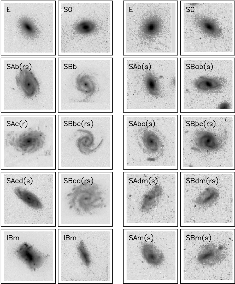
Figure 7: Sample images for galaxies with weighted mean revised Hubble types. The two columns on the left are taken from a sample of local galaxies with types from the RC3, and the two on the right are taken from a sample of distant galaxies imaged with WFPC2 in F814W and types from SCO+RAW+SHC (see text). The nearby galaxy images have been processed to yield $S/N$ and resolutions measures to those comparably found in HST images. The common morphological structures described by the RHS are seen in both samples of galaxy images.

Using the systematic corrections and sample weights derived for the HST classification sets we have compiled a catalog of weighted mean revised Hubble types for our distant galaxy samples. In this way we produce not only a final catalog of higher quality types compared to that from any single classifier, but we are able to derive error estimates for each galaxy. This last point is important from the point of view of assessing the quality of any automated morphological classifier. Galaxies whose morphological properties are uncertain to a number of human classifiers are most likely peculiar in some aspect and hence should not be included in the training or testing of a generic machine classifier. Weighted mean types and errors for our local galaxy sample were adopted from the RC3. Representative galaxies from each of these samples, broken into stage and family groups, are shown in Figure 7.

3.1 A high weight set for family and variety classification

Although agreement between stage classifications was found to be quite satisfactory for developing adequate test/train samples for automatic stage classifiers, the uniformity of the family (barred vs. unbarred) and the variety (ringed vs. non-ringed) classes was less than satisfactory. From the HST image samples, all 3 classifiers agreed on the family assignment only 30% of the time and on the variety assignment only 25% of the time. This is clearly due to a lack of the $S/N$ and resolution required for such morphological classification in galaxy images. In reality, some of the ground-based images also lacked sufficient $S/N$ to allow for the unambiguous assignment of family and variety assignment. Hence, for the purposes of developing a robust morphological classifier capable of dealing with these image properties we chose to develop a third, higher weight set of galaxy images. During the course of a large program to acquire photometric calibration fields for the Digital Palomar Sky Survey (Gal et al. 2000) one of us (SCO) initiated a program for non-photometric conditions of imaging large, bright well-classified galaxies from the list of ”best-classified” galaxies in Buta et al. (1994). These galaxies had classifications agreed upon by several human experts and in fact represent proto-types of the various Hubble stages. Each galaxy was imaged in Gunn gri or Cousins B for 10 to 15 minutes with the Palomar 60-inch using CCD13. Conditions were generally not photometric, but thin cirrus and seeing no worse than 2.5 arcsec FWHM was tolerated for this program. When possible, multiple images of the same galaxy were obtained so that we might characterize how accidental errors in the surface photometry will affect output from the automated morphological classifier. In Table  3 we summarize 30 images in Gunn g and Cousins B of 20 different galaxies selected for experimenting with with automated family and variety classification.

4 PRACTICAL APPLICATION OF THE METHOD

Here we describe the application of the method to a set of HST archival images. Using the results of Section 2, we assembled samples of local and distant galaxies having weighted mean stage estimates and family classifications that at least two human classifiers agreed upon. We show a representative sample of these galaxies in Figure 7. As we shall discuss below, the criteria for building a family classifier training set had to be somewhat liberal in order to compile a usable experimental sample. For stage classification, a series of backpropagation networks using different input parameter vectors and network layer architectures were experimented with. In the case of the family classifier, we used two different types ANN classifiers: a backpropagation-trained feed forward network, and a difference boosting neural network (DBNN) developed by Philip et al. (2000).

4.1 Stage Classification

A set of 262 images were collected using the sample of galaxies having $b/a>0.4$ and weighted mean stage estimates from the analysis of Section 3. Most galaxy classification systems provide criteria for estimating the morphological type of an edge-on system, however because we are concerned here with the analysis of two-dimensional morphological structures, we chose to exclude such high-inclination systems. An LMORPHO task was used to perform automated surface photometry of each image, and then an interactive mosaic viewer was used to inspect the ellipse fit to the low surface brightness isophote in each galaxy postage stamp image. This was done to verify that no improper image processing errors occurred due to confusion from nearby images or other image defects. Ten galaxy stamps were rejected in this step, the majority of these being relatively faint HST-observed galaxies that extended too close to the edge of the WFPC2 field. The human classifiers dealt well with ”masking” such edge effects when the visual classification of Section 2 was performed, however the sky fitting and surface brightness contouring routines of LMORPHO were unable to properly handle such situations. Future automated morphological surveys will of course have to deal more effectively with this type of error, but for the purpose of this work we chose to simply delete these galaxies from any machine classification experiments.

For each of the 252 postage stamp images of well-classified galaxies remaining in our experimental sample the full set of morphologically-dependent Fourier image parameters discussed in Section 3 were computed with LMORPHO. A series of backpropagation neural networks were trained following the procedures outlined in Odewahn (1997) using 3 different types of input vector sets and 6 different network architectures. In every training case, two hidden layers of the same size were used to map n-dimension input vectors to an 8-node output layer, one node for each 2-step interval of the stage axis of the RHS. In practice, a final type was assigned for each input vector using the weighted mean value of the output node value. This allows one to assign not only the highest weight classification, but the rms scatter in this node-weighted mean value can be used to assign a classification confidence. Hence, while any output pattern will result in the assignment of an estimated type, patterns where most of the output signal is carried in one major node will have a high confidence assignment, and patterns where the output pattern is distributed over many nodes will be assigned low confidence.

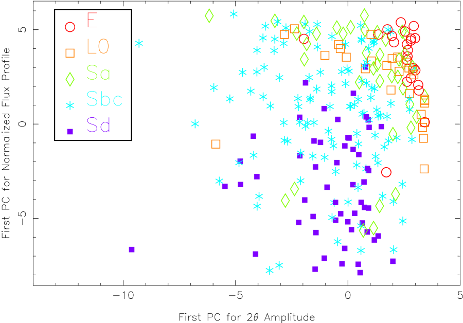
Figure 8: The first principal components formed from an analysis of the $2\theta$ amplitude and normalized flux profiles from 246 local and distant galaxies. We see a clear segregation by revised Hubble stage (normally referred to as the Hubble type). A variety of independent and similarly fuzzy Fourier-based image parameter may be combined via the ANN classifiers described in the text to predict stage values.

The image parameter catalogs were collected into a single binary catalog which can be used in LMORPHO to interactively generate symbol-coded parameter space plots like those shown in Figures  8 and  9. With this package the user can quickly view many different parameter spaces and judge which one shows the largest degree of type separation (whether stage or family) by determining how well the different type-coding symbols are separated in the plot. An important feature in this graphical tool is that any point may be marked and used for a variety of uses. In one mode the user can choose to view on a real-time basis the galaxy image of any selected data point. In this way one is able to determine if a particular outlier is due to improper image processing or some truly unique morphological circumstance. In the latter case, such data are retained for use in classifier training. In the former, these patterns would be rejected from use in gathering training and testing samples. As the images used in this particular series of classification experiments were generally of high quality, fewer than 5% of the original 252 postage stamps were rejected in this manner. For only a few hundred galaxy images (or even less than a few thousand) this process of parameter space inspection is trivial to complete in a few minutes. Finally, we made a preliminary set of ANN training runs using different input parameter sets as well as subdividing the training/testing data in different subsets. Through this process we uncovered an additional 28 objects that consistantly gave highly discrepant training results, i. e. the image parameter combinations for these sources were highly abnormal compared to the bulk of the data, and these sources were rejected from further experiments. This represented about 9% of our original training set, but determining the source of peculiarity for these galaxies will require a larger, more diverse collection of images for future experiments. We determined a number of useful input parameter combinations that showed good segregation by morphological type and a series of different image parameter set patterns were formulated. Each type of pattern would form the input layer to an ANN classifier. For clarity, we assigned a running integer value to each type of input, and we refer to this as the feature set number. We indicate the feature set number for each training exercise in column 8 of Table 6.

In Table 4 we summarize the LMORPHO image parameters that were selected for the stage and family classifiers developed in this paper. Since different image parameters are used in each classifier, we list in column 2 the feature set number for each input pattern using each image parameter.

The selection of training and testing samples was carried out in the same manner for all input vector types. As summarized in Table 5 all galaxies were binned into the 8 type bins corresponding to the 8 nodes of the ANN output layer. Each such bin was divided into two sets: one for training and one for testing. One is always tempted to use more galaxies in the training sample so that the network has a larger number of patterns for generalizing the problem. One danger in backpropagation training is over-training: beyond some number of training iterations the network weights could be adjusted so as to simply memorize the training pattern sets as opposed to generalizing the mapping of input vectors to output classes. To prevent this, one should use an independent test data set to judge classifier performance. The backpropagation code in LMORPHO computes classifier statistics for both a training sample and a testing sample at each user-specified iteration in which the updated ANN weights are stored. In a post-training phase, each set of statistics is inspected by the code to determine the optimal training cycle. The algorithm used to isolate this iteration uses the slope and rms scatter of the correlation between the target stage prediction and the ANN stage prediction. Both the training and testing data sets are used. The case of over-training is detected by a progressive drop in the rms scatter for the training data with a flat or even increasing rms scatter for the test sample. An optimal training cycle is selected that minimizes the rms scatter for training data before over-training occurs. Additionally, the slope of the linear regression must be close to unity within some user-specified tolerance, usually set at 20%.

We summarize the results of our backpropagation training to develop Fourier-based ANN classifiers in Table  6. The slope ($\alpha$) and scatter ($\sigma_{1}$) about a linear regression between the ANN-predicted and the targeted mean Hubble stage are tabulated for both the training and testing data sets for the selected optimal training epoch. Additionally, as with the type comparison analysis in Section 3, we compute a scatter ($\sigma_{2}$) based on direct differences between the ANN and target values following Odewahn and de Vaucouleurs (1993). This statistic reflects more honestly the scatter to be expected for the user of such an ANN-derived catalog. As expected, scatter among the training data is systematically lower than for the test data, since the error function being minimized in the backpropagation training is formed with the training data. However, the scatter derived for the test data is usually about 2-steps on the RHS stage axis, and hence very reasonable for most scientific pursuits with morphological data.

In Figure 10 we compare mean neural network classifier types from 3 different ANNs (marked with asterisks in Table  6) to weighted mean visual types for two sets of data: the training data and the testing data. To summarize, the test data, comprised of sets of input classification parameters and their corresponding target types, were never presented to the ANN classifiers during backpropagation training to establish the network weight values. As such, this data sample represents a fair comparison by which we can judge true network performance. We include in Figure 10 the same correlation for the training sample. In summary, the Fourier-based stage classifiers developed in this experiment clearly perform as well as a human classifier. These results are certainly encouraging if our goal is simply to estimate revised Hubble types for a large number of digital images, but a more important point must be stressed. We have shown that our method of parameterizing a galaxy image preserves the information content needed to emulate the process used by a human classifier. As with the bar classification work described below, our ultimate goal will be to use such a digital image analysis to search for more direct correlations among galaxy properties and ultimately develop a more physically meaningful classification system beyond the RHS.

4.2 Family Classification

As discussed in Section 3, the visual classifiers divided the family estimates into the three bins of the RHS: A, AB, B. The difference between each class is somewhat vague and subject to personal bias. It is not surprising that we found very few cases where all three classifier agree that a galaxy was of the AB family class. As was discussed for Figure 3, the Fourier profiles for AB galaxies are, in the mean, intermediate between the A and B galaxies. However, the AB galaxies show a markedly large variance which is probably due to the wide variance in AB classification criteria used by the human classifiers. The presence of such uncertainty made it impossible to train an effective 3-division stage classifier. For the present work, we approached the problem using an unambiguous set of A and B galaxies and attempted to develop a robust classifier for identifying them using the Fourier-based eigenvector approach discussed in Section 3. When larger samples of morphologically classifiable galaxy images are collected, it is anticipated that a more thorough study of bar strength parameters will allow the development of a more sophisticated automated family classifier.

For the present set of classification experiments we gathered images of 71 A galaxies and 61 B galaxies drawn from the analysis of Section 3. In this case, any galaxy which had family classifications that were agreed upon by at least 2 of the 3 human classifiers were adopted for use. To clarify the problem, we used only A and B classes for classifier experiments. After a series of parameter space inspections, such as those described in the stage classification section, we chose to use the first principal components of the $2\theta$ and $4\theta$ amplitude profiles. We found that additional discrimination was added in many cases using the first principal component of the $4\theta$ phase profile and adopted this for use in the classifier input vector. It was found that including parameters that are highly correlated with bulge to disk ratio (i. e. the principal components of the normalized flux profile) did not add significantly to detecting the presence of a bar. This was surprising in that it is well known that bar shapes and properties are correlated with Hubble stage, and hence bulge to disk ratio (Elmegreen and Elmegreen 1986). In future work with much larger samples of galaxies, the use of terms related to the shape of the surface brightness profile may prove useful for this reason: pattern classifiers can better interpret the meaning of morphological shape parameters like the first principal components of the $2\theta$ and $4\theta$ amplitude profiles if some information related to Hubble stage is provided. For the present small sample of potentially useful training samples, we decided to exclude the use of surface brightness profile shape parameters for the training of a family classifier.

We added two simple global image parameters that contribute information about bar presence that were independent of the Fourier model approach. In determining the shape and orientation of the optimal elliptical aperture for measuring each galaxy, LMORPHO computes a series of ellipse fits to progressively fainter surface brightness levels. The initial surface brightness levels are high and generally sample the bright inner region of a galaxy where the bars are found. It was found that simple parameters using these elliptical isophote parameters could be formed that gave useful information about the presence of a bar that would be independent of the image models derived with the Fourier method. We define the minimum axis ratio of the series of ellipse fits to be $B_{P1}$, and the axis ratio of the largest ellipse (i.e. the fit to the lowest surface brightness level) to be $B_{P2}$. In general, a barred galaxy will have $B_{P1}<B_{P2}$, but with the condition that the major axis length of the isophote measured for $B_{P1}$ is significantly smaller than that measured at the isophote for $B_{P2}$. To discriminate this condition we formed the parameter $B_{P3}=r_{1}/r_{2}$, where $r_{1}$ is the semi-major axis length measured at $B_{P1}$ and $r_{2}$ is the semi-major axis length measured at $B_{P2}$. Additionally, we formed $B_{P4}=B_{P2}/B_{P1}$, to measure the contrast of the ellipticity variation in the galaxy image. It was found that for many galaxies, a plot with $B_{P4}$ on the y-axis and $B_{P3}$ on the x-axis places B galaxies in the upper left corner and A galaxies in the lower right corner. Of course, there is a rather substantial overlapping zone in the low $B_{P4}$ and low $B_{P3}$ region of this plot. Hence, while such a simple scheme can not discriminate all A,B galaxies, it can provide high weight information for some systems. Simple initial ANN classification experiments provided evidence that these parameters, when added to the Fourier-based parameters, produced better discrimination for A,B samples and hence we included them in the training of our final family classifier.

Two types of family classifiers were trained with the input vector parameters shown in Table 4. First, the backpropagation network code used the previously discussed stage classifiers was used to train a network consisting of 2 hidden layers having 12 nodes each. This network mapped an 8-element input vector to a 2-node output layer. Patterns with more power produced in output node 1 were classified as A, and patterns with more power produced in output node 2 were classified as B. Many of the dimensions in this 8-dimensional classification space produce a good split between the A and B populations and hence the backpropagation training converged relatively quickly. As with the stage classifiers, a sample of pure test patterns was retained and used to assess network performance at each stage in the backpropagation weight update process. This procedure gives us a truly independent check on the classifier performance and an effective means of guarding against over-training. A total of 30 training epochs were used in the backpropagation training, and epoch 15 was selected as providing optimal performance with a success rate performance of 92% among training patterns and 85% among test patterns. In a second experiment the DBNN method of Philip et al. (2000) was applied to the identical training and testing patterns as for the backpropagation ANN. After boosting, the training set was found to produce a 94.1% successful classification rate and the test set was found to produce a success rate of 87.5%. The performance of the DBNN classifier was found to be marginally better than the backpropagation-trained network, however a large sample of training data will be needed to assess if this improvement is significant. Nevertheless, both methods produced automated family classifiers that are able to discriminate bar presence with a roughly 90% probability of success.

4.3 Systematic Effects with $S/N$ and Resolution

Image quality plays a crucial role in determining the extent to which morphological classification can be performed on a galaxy. A gradual decrease in image resolution and $S/N$ will systematically degrade the quality of morphological classifications, both by human and machine methods. With stage estimation, one might expect that we lose the ability to differentiate the bulge and disk components, making it extremely difficult to work at the early stage of the Hubble sequence (i. e. differentiate E, S0 and early spiral systems). At the late Hubble stages, we lose many of the low surface brightness features in the out disk regions that are crucial for differentiating among the Sd, Sm and Im systems. With family classification, one can expect that gradual image degradation will make it impossible to detect the presence of a bar, much less characterize the properties of the bar (see van den Bergh 2001). In the past, human classifiers, in particular those dealing with low resolution and low $S/N$ Schmidt plate images (Nilson 1973, Corwin et al. 1985), have generally taken such effects into account by dropping the amount of detail in the literal type assigned to a galaxy. In other words, a system might be classified simply as ”S” rather that ”SBc”, if the image quality is sufficient only to differentiate the difference between early-, mid-, or late-type galaxy. Such effects must be accounted for in any automated system geared towards the recognition of morphological features. One must know if there is a strong systematic bias towards, for instance, missing bar or spiral features as resolution decreases. Perhaps if such effects are well understood we may hope to correct large statistical samples in some systematic way. At the very least, we must quantify the levels of low $S/N$ or resolution that can be tolerated before the quality of automated classifications falls below some minimum tolerance required by a given science goal.

We chose to define resolution as the number of pixels in a galaxy image contained within the isophotal ellipse used to integrate the isophotal magnitude in LMORPHO. This is a reasonable approach for HST images where, for most filters, each pixel approaches the resolution of the optical image. For ground based images we should use the size of the seeing disk, which is generally several times larger than the pixel size. In our present study all of the ground based images have been block averaged to produce pixel sizes that are comparable to the seeing disk and hence we can use this uniform resolution definition for all of the galaxies analyzed. As for defining the $S/N$ in a galaxy image we used two approaches. In the first, we simply compute the ratio of the mean signal (above sky) per pixel to the standard deviation of the local sky measure. In the second approach, we define the mean signal, $S$, to be the zeroeth order term in the Fourier series fitted to the azimuthal distribution in each model annulus, and the noise, $N$, is the r.m.s. scatter about that fit. This latter approach incorporates the Poisson noise associated with the detected galaxy signal and accounts for large scale structural changes across the azimuthal profile. In practice, the two methods had very different ranges, but were found to be well correlated. The method 1 approach yielded $S/N$ estimates in the range 100 to 1000, and the Fourier-based method produced values in the range of 3 to 20. It was found that the early-type galaxies, having little large scale structure in their images, produced the tightest correlation between these two types of $S/N$ estimators. For practical reasons, we used the more easily computed method 1 values in the image classification experiments described in this section.

To characterize how decreased $S/N$ and resolution will affect the quality of our Fourier-based ANN classifiers, we selected sets of galaxies having extremely high $S/N$ and resolution. These systems were found to be classified correctly by the stage and family classifiers discussed in the previous sections. Most of these images were taken from the ground-based datasets obtained with the Palomar 60^′′ discussed in Section 3, but a few of the highest resolution HST images were also included. For samples having well classified stage and family types, we selected galaxies with images that had at least 2000 pixels contained within the optimal elliptical aperture. These sets of images were then systematically re-sampled using an LMORPHO package designed for this experiment to produce postage stamp images of galaxies having progressively lower $S/N$ and resolution. As this exercise was designed to study the general systematic effects of image degradation on morphological classification, no attempt was made to model the noise properties of a given detector, like WFPC2 or STIS (as in Odewahn et al. 1997). For each re-sampled image, an extra component of gaussian noise was added to the original image. We modeled decreasing resolution in two ways. First, we consider the case of high sample rate with image blurring, the case typically encountered with ground-based observations of nearby galaxies. In the second, and more relevant case, we considered a low sample rate with high optical resolution, i. e. the image suffers from a high degree of pixelation. To simulate this effect, we simply block averaged the original galaxy images to a lower image sampling rate. This latter effect is well known to anyone who has classified large numbers of distant galaxies on WFPC2 images and is the one, as we will show, which dominates our ability to determine distant galaxy morphological classification.

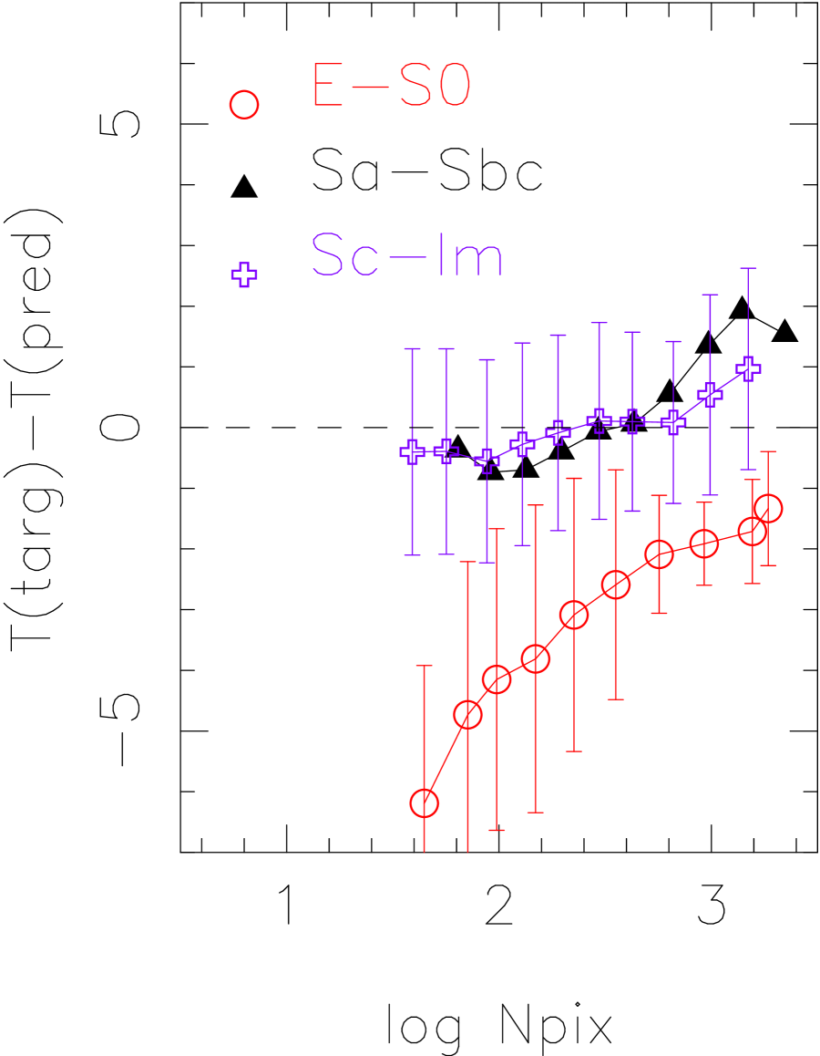
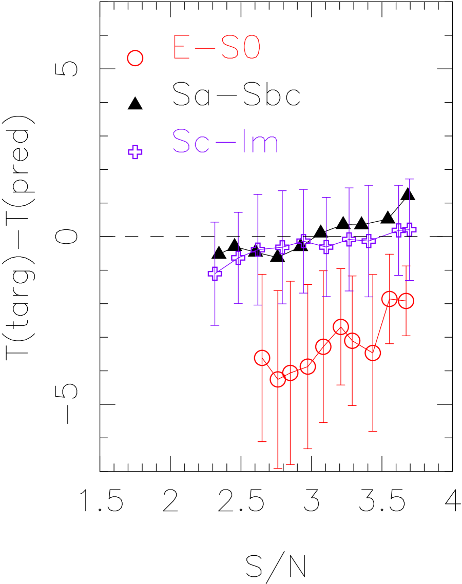
Figure 11: Resolution and $S/N$ in a set of 261 galaxy images have been systematically degraded using repixelation and the addition of a gaussian noise component. The resulting 1901 images were processed with the ANN classifiers discussed in Section 4.2 to estimate Hubble stage. We plot the mean trend in stage residual (target-predicted) for three intervals of target galaxy stage as a function of resolution as measure by the number of image pixels (left) and $S/N$ (right). In each case we have used overlapping x-axis bins of width 0.2 dex to demonstrate the smooth degradation in classifier performance as image quality is lowered. Spiral and irregular stages show a moderate trend in positive mean offset (ANN classifies earlier) and increased rms scatter with decreasing resolution and $S/N$ . The E+S0 systems, as one expects from viewing Figure 10, exhibit a mean negative offset (ANN classifies later) of 2-3 Hubble steps at even the best image quality for the present samples. Additionally, this mean offset and increasing rms scatter in T-types is clearly steeper than for spiral and irregular galaxies.

The results for the backpropagation ANN stage classifiers are summarized in Figure 11. For this experiment a simple success rate calculation was not appropriate. We desire to know not only whether a classifier fails to predict the correct stage estimate within some number of type bins, but in which direction a misclassification occurs. If the classifier consistently pushed stage estimates in an early (towards E,S0) or a late (toward Im) direction then a substantial bias will be introduced in the scientific interpretation of the ANN-generated morphological catalog. Hence, we chose to compute the trend in type stage residuals, computed in the sense of $T(target)-T(ANN)$, as a function of resolution and $S/N$ , where $T(target)$ is the true galaxy type. These trends were computed using overlapping bins in resolution or $S/N$ , with the mean stage residual and the rms about that mean computed in each bin. A set of 1901 re-sampled images were processed with the ANN classifiers discussed in Section 4.2 to estimate Hubble stage. In Figure 11 we show trends in stage residuals for three sets of target stage intervals: E-S0, Sa-Sbc, and Sc-Im. In each case we have used overlapping x-axis bins of width 0.2 dex, and we expect to observe the degradation in classifier performance as image quality is lowered. Spiral and irregular stages show a moderate trend in positive mean offset (i. e. the ANN classifies these galaxies with an earlier value) and increased rms scatter about the mean with decreasing resolution and $S/N$ . Of more significance, E+S0 galaxies exhibit a mean negative offset (i. e. the ANN classifies these systems to be later than the target value) of 2-3 Hubble steps. This occurs for even the highest resolution and highest $S/N$ galaxy images in our present sample. Additionally, this mean offset and increasing rms scatter in T-types for the E+S0 galaxies is clearly steeper than for spiral and irregular galaxies. A variety of network architectures and input parameter vectors were experimented with in order to correct this problem. Little improvement was obtained due in large part to the lack of a sufficiently large sample of images for such galaxies. As discussed in Cohen et al. (2001), E+S0 in the field are relatively rare for $I_{814}$ ${}_{<}\atop{{}^{\sim}}$22, and hence a very large number of HST parallel observations are needed to build up a significant image library. Work is currently underway to collect such images from the many archival HST observations of moderate-redshift clusters. Clusters contain not only a large number of galaxies in a single WFPC2 field, but the morphological fractions of these galaxies are skewed to the early-types. The analysis of such large samples will potentially eliminate the mean negative stage offsets observed for the E+S0 samples of Figure 11, however it is doubtful that we can hope for a comparable decrease in the rms of such stage classifications in the low $S/N$ and resolution regimes. It is clear that images of sufficiently high quality are needed to differentiate many of the subtle structural properties of early-type galaxies, as is clear from the work of Im et al. (2000). The larger field size, higher quantum efficiency, and especially increased resolution of ACS, compared to WFPC2, will make this the instrument of choice on HST for identifying large samples of moderate-redshift E+S0 systems in the near future.

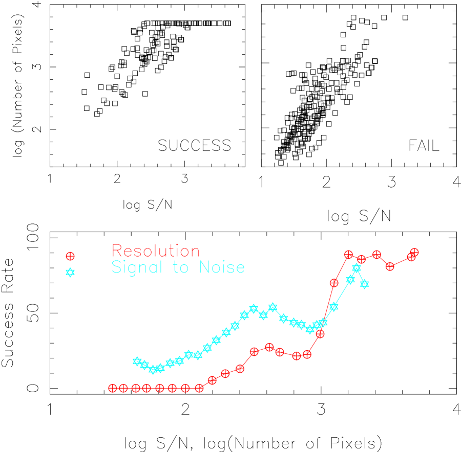
Figure 12: The resolution and $S/N$ of a set of excellent quality images of clearly barred galaxies (family=B) have been systematically degraded to produce trends in $S/N$ vs. resolution (as measured by number of pixels) for the cases of classifier success (left) and failure (right). The resulting mean trends in classifier success with $S/N$ (star) and resolution (cross) are shown in the lower panel.

The results for the backpropagation ANN family classifier are summarized in Figure 12. Unlike the stage classifiers, our family classifiers predict only two states: A or B. Hence, we are able to characterize the output results as success or failure cases. We therefore chose to plot the distribution of $S/N$ and resolution for ANN-predicted classes for a sample of barred galaxies that agree with the target value and for those that fail to agree. As expected, in Figure 12 the success cases cluster in the high $S/N$ , high resolution area of the plot, and the failure cases cluster most heavily in the low $S/N$ and resolution region. For clarity, we also plot the success rate trends binned by $S/N$ and resolution. For identifying the presence of a bar, it is quite clear from these mean relations that some critical image resolution is required. For our present samples and Fourier-based ANN classifiers, we are unable to effectively identify barred systems at better than a 70% success rate until we obtain galaxy images with at least 1000 resolution elements ($\log N_{pixels}$ ${}_{>}\atop{{}^{\sim}}$3, where $\log N_{pixels}$ is the number of image pixels above the isophotal threshold). The trend with $S/N$ is less steep, but a mean $S/N$ (per pixel) of around 1000 is also required to reliably identify bars. The same experiment was carried out for a sample of unbarred (A) galaxies with different, but expected, results. In this case, galaxies that are successfully classified as A at high $S/N$ and resolution generally retain that classification at low $S/N$ and resolution. In other words, the ANN classifiers rarely turn A galaxies into B galaxies, as is true for human classifiers. In general, as we lose image resolution we begin to loose the ability to identify morphological bars, but we do not tend to contaminate B galaxy samples with misclassified A galaxies, an important point when considering the the frequency of barred systems at high redshift.

5 SUMMARY

In this work we have developed a methodology for classifying galaxies based on the strength of Fourier components in the azimuthal light distribution. We have used pattern recognition techniques to develop machine classifiers which map the Fourier mode information to the revised Hubble system, a well known galaxy classification system. We must stress that the basic motivation here is not simply to create a machine-based replication of the revised Hubble system. The RHS was developed to describe a variety of properties, some of which are directly related with two-dimensional morphological structures in galaxies. We therefore have chosen to use this classification system to guide our development of new quantitative classification systems. We have demonstrated here a method of extracting galaxy image information in a way which permits us to automate the recognition of bars and Hubble type, as defined by the family and stage axes of the RHS.

In a sense, this work represents a proof-of-concept study. The current method is able to recognize many of the same structural properties of galaxies that have guided the study of galaxy morphology for the last fifty years. Having established how well the method works, under a variety of image $S/N$ and resolution regimes, we can entertain the prospect of searching for refinements in the classification system itself. In other words, the next step is to apply various multivariate statistical techniques and non-supervised learning methods to determine if there are relationships among the Fourier-based model image parameters that convey more directly relationships among galaxies. For instance, strength of the $2\theta$ and $4\theta$ Fourier components in the inner regions of disk galaxies might be used to form a continuous measure of bar strength, and we might dispense with the 3-cell family axis of the RHS all together. Continuity along each axis of RHS was recognized long ago (de Vaucouleurs 1959), but human classifiers lacked the image measurement ability to classify galaxies in anything other than a set of bins. In addition, as discussed in Section 4.3, we may now incorporate information on image quality, as measured by $S/N$ and resolution, in determining what measurable morphological information is available in a galaxy image.

Finally, disk systems in the late stages of the RHS show increasing amounts of global image asymmetry. Such asymmetries are sometimes linked to tidal encounters with nearby galaxies. How are these asymmetries related? Is the increased degree of disk asymmetry caused exclusively by encounters, and is the high frequency of asymmetric systems observed at $z$ ${}_{>}\atop{{}^{\sim}}$0.5 the result of an increased interaction rate? Strength of the $1\theta$ Fourier component, as measured by the first principal component of the $1\theta$ amplitude profile, may be used to measure this asymmetry independent of the presence of other morphological structures like bars and arms, something that is not possible with less sophisticated image-rotation asymmetry measurements. Such asymmetry measurements may be correlated closely with the internal kinematics of the galaxy (Rix & Zaritsky 1996) or the present level of active star formation in a disk and hence will convey more direct insight into the physical processes driving galaxy formation and evolution.

We acknowledge support from NASA grants AR.6385.01.95A, GO-6609.01-95A, and AR-7534.01-96A.

REFERENCES

Abraham, R., Tanvir, N.R., Santiago, B., Ellis, R. S., Glazebrook, K. G. & van den Bergh, S., 1996, MNRAS, 279, L47

Abraham, R., Valdes, F., Yee, H., & van den Bergh, S. 1994, ApJ, 432, 75

Andreon, S., Gargiulo, G., Longo, G., Tagliaferri, R., Capuano, N. 2000, MNRAS, 319, 700

Bazell, D. 2000, MNRAS, 316, 519

Bertin, E., & Arnouts, K., 1997, A&A, 124, 163

Bender, R. & Mollenhoff, C. 1987, A&A, 177, 71

Buta, R. 1987, ApJS, 64, 383

Buta, R. & Combes, F. 1996, Fund. Cosmic Physics, 17, 95

Buta, R., Mitra, S., de Vaucouleurs, G., & Corwin, H.G. 1994, AJ, 107, 118.

Cohen, S. H., Windhorst, R. A., Odewahn, S. C., Chiarenza, C. A. T., & Driver, S. P. 2001, AJsubmitted

Southern Galaxy Catalog (University of Texas Monograph in Astr., No.4)

Corwin, H. G., de Vaucouleurs, A. & de Vaucouleurs, G. 1985, Southern Galaxy Catalog (University of Texas Monograph in Astr., No.4)

de Vaucouleurs, G., de Vaucouleurs, A., Corwin, H.G., Buta, R., Paturel, G. & Fougué, P. 1991, The Third Reference Catalog of Bright Galaxies, Springer Verlag: New York (RC3)

Driver, S. P., Windhorst, R. A., & Griffiths, R. E. 1995a, ApJ, 453, 48

Driver, S. P., Windhorst, R. A., Ostrander, E. J., Keel, W. C., Griffiths, R. E., & Ratnatunga, K. U. 1995b, ApJ, 449, L23

de Vaucouleurs, G. 1977, The Evolution of Galaxies and Stellar Populations, ed. B. Tinsley and R. Larson, 43, (New Haven, USA:Yale University Press)

de Vaucouleurs, G. 1958, Rev. Modern Phys., 30, 926

de Vaucouleurs, G. 1959, Handbuch der Physik, 53, 311

de Jong, R. S., & van der Kruit, P. C. 1994, A&AS, 106, 451.

Elmegreen, B., & Elmegreen, D. 1985, ApJ, 288, 438

Frei, Z. et al. 1996, AJ, 111, 174

Gal R.R., de Carvalho, R.R., Brunner, R., Odewahn, S.C., & Djorgovski, S.G., 2000, AJ, 120, 540

Glazebrook, K., Ellis, R. E., Santiago, B., & Griffiths, R. E. 1995, MNRAS, 275, L19

Hickson, P. 1993, Astrophysical Letters and Communications, 29, 1

Hubble, E. 1926, ApJ, 64, 321

Kent, S. 1986, AJ, 91, 1301

Lauberts, A., and Valentijn, E.A., 1989, The Surface Photometry Catalogue of the ESO-Uppsala Galaxies (European Southern Observatory, Garching)

Lauer, T. 1985, ApJS, 57, 473

Mahonen, P. H. & Hakala, P. J. 1995, ApJ, 452, L77

Mahonen, P. & Frantti, T. 20001 ApJ, 541, 261

Naim, A., Lahav, O., Sodre, L., & Storrie-Lombardi, M. C. 1995, MNRAS, 275, 567

Naim, A., Ratnatunga, K. U., Griffiths, R. E. 1997, ApJ, 476, 510

McClelland, J. L. & Rumelhardt, D. E. 1988, Explorations in Parallel Distributed Processing, (MIT Press), Cambridge, MA

Nilson, P. 1973, Uppsala General Catalog of Galaxies, Roy. Soc. Sci., Uppsala (UGC)

Philip, N. S, Joseph, K. B., Kembhavi, A., & Wadadekar, Y 2000, Proceedings of Automated Data Analysis in Astronomy, Narosa Publishing, New Delhi, 125

Rix, H. & Zaritsky, D. 1995, ApJ, 447, 82

Roberts, M. S. & Haynes, M. P. 1994, ARA&A, 32, 115

Odewahn, S.C. 1997, Nonlinear Signal and Image Analysis, Annals of the New York Academy of Sciences, 188, 184

Odewahn, S.C., Windhorst, R. A., Driver, S. P., & Keel, W. C. 1996, ApJ, 472, L13

Odewahn,S.C., Stockwell, E.B., Pennington, R.M., Humphreys, R.M., and Zumach, W.A. 1992, AJ, 103, 318

Odewahn, S. C, & Aldering, G. 1995, AJ, 110, 2009

Odewahn, S. C. 1995, PASP, 107, 770

Odewahn, S.C., Stockwell, E.B., Pennington, R.M., Humphreys, R.M., & Zumach, W.A. 1992, AJ, 103, 318

Odewahn, S.C. 1989, Properties of the Magellanic Type Galaxies, Ph.D. thesis, Univ. of Texas

Ohta, K, Hamabe, M., & Wakamatsu, K. 1990, ApJ, 357, 71

Simien, F & de Vaucouleurs, G. 1986, ApJ, 302, 564

Spiekermann, G., 1992, AJ, 103, 2102

Storrie-Lombardi, M.C., Lahav, O., Sodre, L.J., and Storrie-Lombardi, L.J. 1992, MNRAS, 258, 8

van den Bergh, S., Cohen, J. G., & Crabbe, C. 2001, AJ, 122, 611

Weir, N., Fayyad, M. F., & Djorgovski, S. 1995, AJ, 109, 2401

Whitmore, B. C. 1984, ApJ, 278, 61

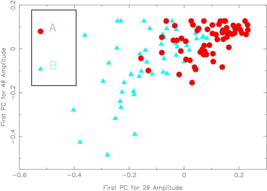
Figure 9: The first principal components formed from an analysis of the $2\theta$ and $4\theta$ profiles from 205 local and distant galaxies. We see a fuzzy segregation by revised Hubble family (barred vs. unbarred). The unbarred (A) galaxies preferentially occupy the upper region of this space. The AB galaxies cover an intermediate region of this parameter space, and for clarity we plot only the A and B galaxies.

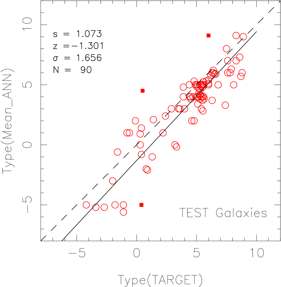
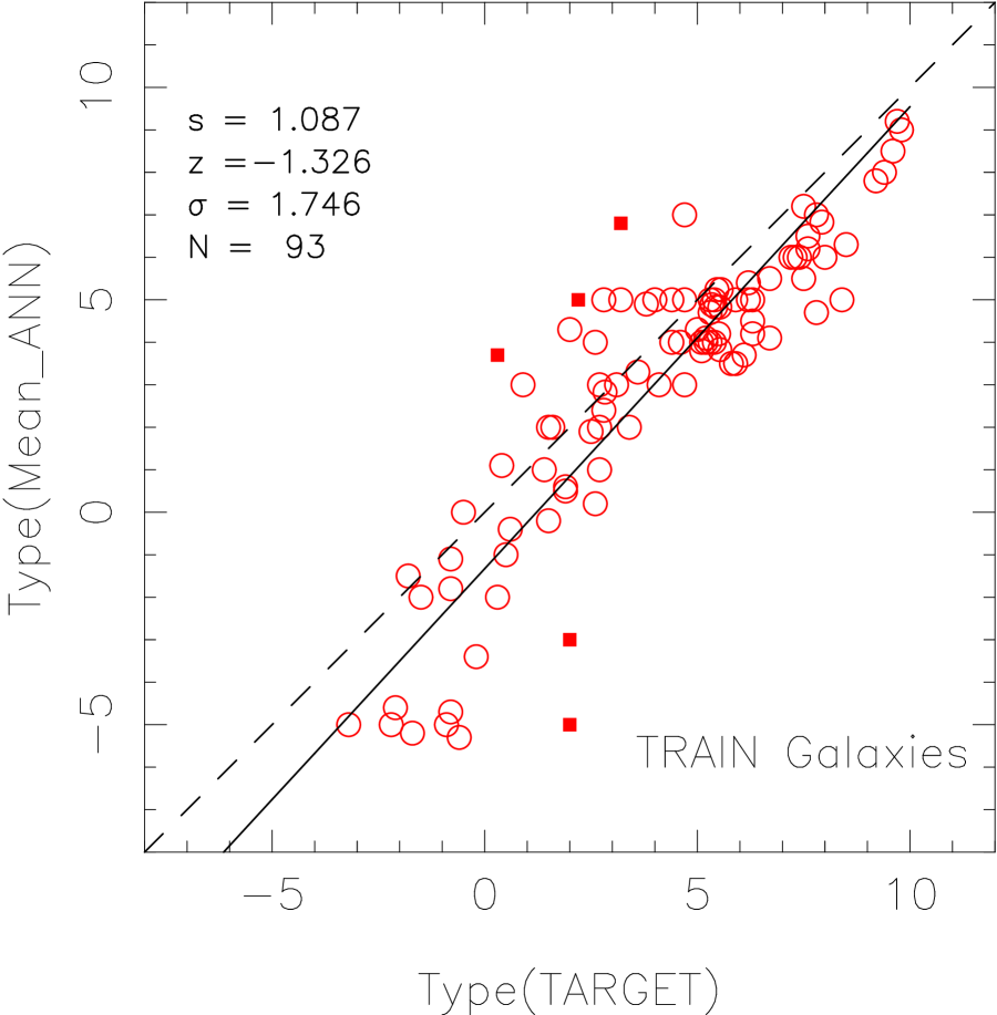
Figure 10: (a) [Left] The mean stage estimates from 4 independently trained ANN classifiers as a function of target type as given by the catalog of weighted mean visual stage estimates. As discussed in the text, each ANN classifier is fed a combination of principal components based on an eigenvector analysis of Fourier amplitude profiles. The linear regression indicated by the solid line departs systematically from the dashed unity line but gives a reasonable y-axis residual scatter of 1.6 steps on the 16-step revised Hubble stage axis. [Right] The same correlation with the exception that we plot only data from galaxies used as input patterns during backpropagation training to establish ANN weight values. In both cases, the the small box symbols are data rejected after two cycles of 3-sigma rejection in the linear regression fit.

Table 1: Results of Human Classifier Stage Comparisons

$T_{x}$	$T_{y}$	S	a	b	R	N	$\sigma$
SCO	RC3	L	1.00$\pm$0.05	0.022$\pm$0.148	0.898	119	1.60
SHC	RC3	L	0.98$\pm$0.06	0.089$\pm$0.213	0.810	123	2.13
RAW	RC3	L	1.02$\pm$0.05	-0.060$\pm$0.159	0.889	121	1.61
SHC	SCO	L	1.00$\pm$0.08	-0.083$\pm$0.275	0.739	123	2.53
RAW	SCO	L	1.00$\pm$0.04	0.060$\pm$0.118	0.929	120	1.38
RAW	SHC	L	1.02$\pm$0.07	-0.077$\pm$0.240	0.792	121	2.21
SCO	HST1	D	1.02$\pm$0.04	0.045$\pm$0.087	0.911	117	1.92
SHC	HST1	D	0.99$\pm$0.07	-0.011$\pm$0.161	0.786	125	2.86
RAW	HST1	D	0.98$\pm$0.06	-0.107$\pm$0.154	0.810	137	2.73
SCO	SHC	D	0.99$\pm$0.07	0.113$\pm$0.148	0.795	116	2.84
RAW	SCO	D	0.99$\pm$0.06	0.114$\pm$0.117	0.860	113	2.41
RAW	SHC	D	0.99$\pm$0.08	-0.046$\pm$0.201	0.729	123	3.27

The first two columns indicate the stage catalogs used on each axis to fit the relation $T_{y}=aT_{x}+b$. The column labeled S indicates whether a sample of local (L) or distant (D) galaxies were used. The correlation coefficient, R, the number of galaxies in the fit, N, and the standard deviation of the stage residuals, $\sigma$ are also tabulated.

Table 2: Accidental Stage Errors by Classifier

Sample	RC3	HST1	SCO	RAW	SHC
Local	$0.97\pm 0.35$	-	$1.26\pm 0.26$	$0.88\pm 0.39$	$2.02\pm 0.16$
Distant	-	$1.53\pm 0.13$	$1.20\pm 0.13$	$2.16\pm 0.09$	$2.48\pm 0.08$

Table 3: The Palomar Galaxy Sample

name	RC3 Type	filters
NGC 1744	SB(s)d	1g
NGC 4501	SA(rs)b	2B
NGC 4519	SB(rs)d	1g
NGC 4618	SBm	2g
NGC 5850	SB(r)b	1g,1B
NGC 5985	SAB(r)b	1g
NGC 5377	SB(s)a	1g
NGC 6070	SA(s)c	3g,1B
NGC 6340	SA(s)0	1g
NGC 6384	SAB(r)bc	1g,2B
NGC 6643	SA(rs)c	1g
NGC 6764	SB(s)bc	1g
NGC 6824	SA(s)b	1g
NGC 6951	SAB(rs)bc	2g
NGC 7217	SA(r)ab	2g
NGC 7457	SA(rs)0	1g
NGC 7479	SB(s)c	1g
NGC 7741	SB(rs)cd	1g
PGC 61512	SB(s)dm	1g

Table 4: LMORPHO Image Parameters Used for Classification

name	Feature Set	Comment
PC1_Fnorm	1,2,3	First PC of normalized flux profile
PC2_Fnorm	1,2,3	Second PC of normalized flux profile
PC1_1TA	2,3	First PC of $1\theta$ amplitude profile
PC1_2TA	1,2,3,4	First PC of $2\theta$ amplitude profile
PC2_2TA	1	Second PC of $2\theta$ amplitude profile
PC1_4TA	1,2	First PC of $4\theta$ amplitude profile
PC2_4TA	1,2,4	Second PC of $4\theta$ amplitude profile
PC1_4TP	1,2	First PC of $4\theta$ phase profile
PC2_4TP	1,2,4	Second PC of $4\theta$ phase profile
S/N	3	Mean $S/N$ measured in elliptical aperture
$N_{pix}$	3	Number of image pixels
$B_{P3}$	4	Bar parameter 3
$B_{P4}$	4	Bar parameter 4

Table 5: Train/Test Galaxies Divided by Stage

node number	Number	T interval	Literal range
1	19	-8.0 -4.5	E to E0-1
2	6	-4.5 -2.5	E+ to L0-
3	13	-2.0 -0.5	L0 to L0+
4	18	-0.5 1.5	S0a to Sa
5	34	1.5 3.5	Sab to Sb
6	91	3.5 5.5	Sbc to Sc
7	30	5.5 7.5	Scd to Sd
8	12	7.5 10.5	Sdm to Im

Table 6: Results for Backpropagation ANN Stage Classifiers

$\alpha^{TR}$	$\sigma_{1}^{TR}$	$\sigma_{2}^{TR}$	$\alpha^{TE}$	$\sigma_{1}^{TE}$	$\sigma_{2}^{TE}$	Epoch	Feature Set	l
0.920	0.93	2.09	0.908	2.25	2.09	5800	1	9
0.953	1.15	1.71	0.968	2.29	1.71	2900	1	11
1.045	1.16	1.68	0.949	2.46	1.68	2600	1	12 $\ast$
0.935	1.20	1.84	0.959	2.37	1.84	2000	1	13
0.705	1.71	2.57	0.722	1.92	2.57	1000	1	14
0.931	1.78	2.28	0.906	1.92	2.28	4200	2	9
0.974	1.35	1.82	0.909	2.06	1.82	4300	2	11
0.936	1.56	2.25	0.914	2.06	2.25	2300	2	12
0.938	1.13	1.87	0.986	2.51	1.87	3900	2	13 $\ast$
1.081	1.32	1.74	1.005	1.88	1.74	3600	2	14
1.009	1.44	1.71	0.978	1.71	1.71	1800	3	9
0.878	1.16	2.59	0.803	1.77	2.59	1000	3	11
1.016	0.93	1.54	0.946	1.83	1.54	900	3	12 $\ast$
0.917	1.36	2.07	0.965	1.62	2.07	500	3	13
1.025	0.79	1.38	1.045	1.79	1.38	900	3	14

Asterisks indicate networks that gave the best performance for a given node architecture and these were used to compute mean types in Figure 10. The TR superscript refers to training results and TE refers to testing results. The l column indicates the number of nodes in each of the two hidden layers used in every ANN. As explained in the text, the Feature Set number indicates the set of image parameters fed to each network.