Dynamical Modeling of the Stellar Nucleus of M31

We present stellar dynamical models of the lopsided, double–peaked nucleus of M31, derived from Hubble Space Telescope (HST) photometry. A Schwarzschild–type method, in conjunction with Richardson–Lucy deconvolution, was employed to construct steadily rotating, hot, stellar disks. The stars orbit a massive dark object, on prograde and retrograde quasi–periodic loop orbits. Our results support Tremaine’s eccentric disk model, extended to include a more massive disk, non zero pattern speed ($\Omega$), and different viewing angle. Most of the disk mass populated prograde orbits, with $\simeq 3.4\%$ on retrograde orbits. The best fits to photometric and kinematic maps were disks with $\Omega\simeq 16\mbox{\,km\, s${}^{-1}$\, pc${}^{-1}$}\,$. We speculate on the origins of the lopsidedness, invoking recent work on the linear overstability of nearly Keplerian disks, that possess even a small amount of a counter–rotating component. Accretion of material—no more massive than a globular cluster—onto a preexisting stellar disk, will account for the mass in our retrograde orbits, and could have stimulated the lopsidedness seen in the nucleus of M31.

1 INTRODUCTION

The nuclei of normal galaxies are thought to harbor massive dark objects (MDOs), which could be supermassive black holes. These central regions often possess dense agglomerations of stars, whose structural and kinematical properties appear to be correlated with global galaxy properties (see Gebhardt et al., 1996; Ferrarese & Merritt, 2000; Gebhardt et al., 2000). The imprint of galaxy formation is surely recorded in the nature of stellar orbits. No more unusual examples are, perhaps, known than the nuclei of the galaxies, NGC4486B (in the Virgo cluster) and M31 (our nearest large neighbor). The proximity of M31 has enabled detailed photometric and kinematic observations of its nucleus, beginning with the detection of its asymmetrical shape by Stratoscope II (Light et al., 1974), and its resolution into a double–peaked structure by the HST images of Lauer et al. (1993). The central peak (P2) lies close to the presumed location of the MDO, located in a small region of UV–bright stars (King et al., 1995; Lauer et al., 1998; Kormendy & Bender, 1999). Tremaine (1995) proposed that the off–centered peak (P1) marks the region in a disk of stars, where lie the apoapses of many eccentric orbits. This lopsided structure is expected to rotate steadily with some pattern speed, and remain locked in place by the self–gravity of all the stars. We construct numerical stellar dynamical models, wherein the disk potential is derived directly—after bulge subtraction—from the HST photometry of Lauer et al. (1998). Model construction and comparisons with data make many demands on computational resources. Hence it was not practical to explore the effects of varying values of many of the parameters concerning the bulge and disk; we take many of these values from Kormendy & Bender (1999). However, we do explore the effect of varying the pattern speed. We state our assumptions and give an outline of our method below.

We assumed that the bulge–subtracted light emanated from a steadily rotating, inclined, razor–thin, flat, disk of stars, in orbit about the MDO. The stars compose a collisionless, self–gravitating system. Hence the orbits of individual stars are governed by the combined gravitational attractions of the MDO, and the smooth, self–gravitational potential of all the stars. A bulge–disk decomposition of the V–band image of Lauer et al. (1998) yielded the disk surface density, from which the smooth disk potential was computed. For some chosen value of the pattern speed ($\Omega$), orbits of test stars were integrated numerically in the rotating frame. A selection of prograde and retrograde (quasi–periodic) loop orbits of various sizes composed an orbit library. The orbits were populated with “stars” ($\sim 237,000$ in all), spaced uniformly in time, and the disk light (in a central region) partitioned into many cells, with more cells than orbits. Determination of orbit masses, from the known luminosities of the cells, required solving an overdetermined problem, involving positive quantities. This was achieved through $\sim 5000$ iterations of a RL algorithm (Richardson, 1972; Lucy, 1974). The entire procedure was repeated for several values of $\Omega$. Comparisons with the kinematic maps of Bacon et al. (2001) followed. Central line–of–sight velocity distributions were calculated to emphasize the regions in velocity space, where retrograde orbits contribute. Following Kormendy & Bender (1999), we assumed a distance to M31 of $770\mbox{\,kpc}$ (on the sky, $1\arcsec$ corresponds to $\simeq 3.73\mbox{\,pc}$), mass of the MDO, $M\,=\,3.3\times 10^{7}\mbox{\,M${}_{\sun}$}\,$, and mass–to–light ratio of the (bulge–subtracted) nuclear disk equal to $\Upsilon_{V}=5.73\,$.

2 MODEL CONSTRUCTION

2.1 Deprojection and Disk Potential

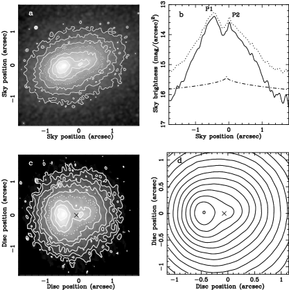
Figure 1: Derivation of the nuclear disk, and its (smooth) gravitational potential. (a) Observed sky brightness distribution, from Lauer et al. (1998); the dotted curve has magnitude $14.3$, and successive isocontours differ by $0.25$ magnitudes. (b) Brightness profiles along the P1–P2 line: observed (dotted curve), the Sérsic bulge (dashed–dotted curve), and the bulge–subtracted nuclear disk (solid curve). (c) Brightness distribution of the disk, viewed face–on; the isocontours follow the same convention as in (a). Isocontours of the disk–potential are displayed in (d); the units are such that the deep minimum near P1 has depth equal to unity, and successive isocontours mark increments of $0.05\,$. In (c) and (d), “X” marks the location of the center of mass.

Fig. 1a shows the nucleus of M31, plotted from the V–band, HST observations of Lauer et al. (1998). The UV cluster and the MDO are at the origin. P2 is near the MDO, with sky coordinates ($0\aas@@fstack{\prime\prime}023,\,0\arcsec$), and P1 is located at ($-0\aas@@fstack{\prime\prime}48,\,0\arcsec$). The bulge was assumed to be spherical, with a Sérsic brightness profile (Sérsic, 1968; Kormendy & Bender, 1999)—see Fig. 1b. The center of mass (COM) of the bulge, disk, and MDO was required to coincide with the bulge center; this common location was determined, by an iterative method, at ($-0\aas@@fstack{\prime\prime}0684,0\arcsec$), in agreement with Kormendy & Bender (1999). With one notable exception, (Bacon et al., 2001), all investigations have assumed that the nuclear disk is coplanar with the much larger galactic disk of M31. We obtained very poor results with this assumption. Therefore, we resolved to determine the inclination and orientation of the nuclear disk, based on the photometry, similar to Bacon et al. (2001). The disk light covered an approximately elliptical region, with a ragged edge. The plane in which the best–fit ellipse (to the edge) deprojected to a circle was defined to be the disk plane; its inclination ($i$), and PA of the line of nodes, were $\simeq 51.54{\degr}$, and $\simeq 62.66{\degr}$, respectively. The face–on view of the disk, shown in Fig. 1c, has mass $\simeq 2.15\times 10^{7}\mbox{\,M${}_{\sun}$}\,$.

To minimize edge–effects, the self–gravitational potential was evaluated in the disk plane, at $10^{4}$ grid points within a central square, of side equal to $2\aas@@fstack{\prime\prime}28$. However, the Newtonian $|{\bf r}-{\bf r^{\prime}}|^{-1}\,$ contributions from the entire disk of Fig. 1c, which has diameter $\simeq 3\aas@@fstack{\prime\prime}6$, was used. The grid values were fit to a $20$–th order polynomial function of the Cartesian coordinates, $\Phi_{d}(\mbox{\boldmath$r$})$, a contour plot of which is displayed in Fig. 1d. The polynomial form smoothed the potential, facilitated coding of the integrator, and checking of the integrated orbits in the nearly Keplerian limit (Sridhar & Touma, 1999). Figs. 1c and 1d can be imagined as either snapshots of a rotating configuration, or as steady images in a frame rotating with some angular speed $\Omega$, about an axis normal to the disk plane, and passing through the COM. The forces on a test star include the gravitational attractions of the MDO and disk, as well as centrifugal and Coriolis forces. The contribution of the bulge was ignored, because it is so much smaller than the other forces.

2.2 The Orbit Library

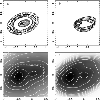
Figure 2: Orbits in the rotating frame and photometric fits. The axes in all panels are sky positions. (a) and (b) show prograde and retrograde loop orbits, respectively, as seen on the sky, for $\Omega=16\mbox{\,km\, s${}^{-1}$\, pc${}^{-1}$}$; the parent (resonant) orbits are overdrawn as the solid curves. The photometry in (c) is from (Lauer et al., 1998), smoothed with a Gaussian beam of FWHM $=0\aas@@fstack{\prime\prime}17\,$. The (bulge–subtracted) light in the region enclosed by the dashed box was employed in our Schwarzschild–type iterative method. (d) is our model disk, including the bulge. The dotted lines in both (c) and (d) have magnitude equal to $14.5$, and successive isocountours differ by $0.25$ magnitudes. The brightness is displayed in the “negative” mode, to better emphasize the distribution.

Orbits were computed in the rotating frame by numerically integrating the equations of motion,

$$\mbox{\boldmath$\ddot{r}$}\;=\;-\frac{GM}{r}\;-\;\mbox{\boldmath$\nabla$}\Phi_{d}\;-\;\Omega^{2}\mbox{\boldmath$r$}\;-\;2\Omega\,\left(\hat{z}\,\mbox{\boldmath$\times$}\,\mbox{\boldmath$\dot{r}$}\right)\,,$$ (1)

using a $4$th–order, adaptive step size, Runge–Kutta scheme. The global structure of orbits was explored by studying Poincaré surfaces of section. The principal families of orbits were lenses and loops. Lens orbits change the sign of their orbital angular momentum (Sridhar & Touma, 1997, 1999). Stars on such orbits will collide with the MDO, in the time it takes an orbit to precess. These time scales do not exceed a million years, even for quite large orbits; dwarf, as well as giant stars on lens orbits will be lost to the MDO (if not tidally disrupted before). Hence lens orbits were excluded from our modeling. Other orbits that were also omitted included chaotic orbits, and those parented by higher order resonances. The loops orbits were of two kinds: prograde and retrograde, some of which are shown in Figs. 2a and 2b; these were the only orbits included in our orbit library. The kinematic model of Tremaine (1995), the Kepler–averaged dynamics of Sridhar & Touma (1999), and studies of slow, linear modes by Tremaine (2001), all suggest the use of the prograde loops as the back bones of the orbit library. The necessity of including retrograde loops is less obvious, and was stimulated by the investigations of Touma (2001). It turned out that the retrograde loops significantly improved fits near P2.

For each value of energy, loops of two or three different “thicknesses” (i.e. deviations from the parent loop) were computed. Each orbit was sampled, and populated with “stars”, spaced apart uniformly in time. All stars in an orbit are accorded the same (unknown) mass; this is not a restriction, because in a collisionless system, the relevant physical quantities are the mass per orbit. The numbers of “stars” in an orbit was chosen proportional to the inverse square of the energy (approximately, square of the “semi–major axis”) of the parent loop; thus $25$ stars sufficed for an orbit with $a=0\aas@@fstack{\prime\prime}02$, whereas an orbit with $a=0\aas@@fstack{\prime\prime}6$ was sampled by more than $10,000$ stars. Altogether, the positions and velocities of $\sim 237,000$ stars, populating $50$ prograde orbits and $20$ retrograde orbits, were recorded.

2.3 Richardson–Lucy Deconvolution

Orbit masses were determined by iteratively imposing on the model, consistency with the bulge–subtracted sky brightness of a region covered by the orbits; the dashed box of Fig. 2c encloses this region. The box was divided into $112$ equal square cells, each of side $0\aas@@fstack{\prime\prime}09\,$; each cell was small enough to give good resolution, and large enough (16 pixels) to keep pixel noise levels low. The “observed” mass per cell, $\mu_{j}$ (for $j=1\ldots 112$), was obtained from the observed light, by multiplication with $\Upsilon_{V}\,$; these numbers composed our basic data. We defined $m_{i}$ (for $i=1\ldots 70$) as the mass of orbit $i$, that also lies within the box; the total mass in the orbit exceeds $m_{i}\,$. We normalized $\sum_{i=1\ldots 70}m_{i}=\sum_{j=1\ldots 112}\mu_{j}=1\,$, to unit mass in the box. A linear relationship, $\mu_{j}\,=\,\sum_{i=1\ldots 70}K(j|i)\,m_{i}$, exists between the “observed masses” $\mu_{j}$, and the unknown masses $m_{i}$. The positive kernel, $K(j|i)$, is known from the orbit library. It has the property, $\sum_{j=1\ldots 112}K(j|i)=1$, for all $i=1\ldots 70$. An initial guess, $\{m_{i}^{\rm g}\}$, was iterated by the RL algorithm (Richardson, 1972; Lucy, 1974). The problem being overdetermined, about $5000$ iterations ensured good convergence to some $\{m_{i}^{\rm f}\}$. Velocities were then transformed to the inertial frame. Rescaling of $\{m_{i}^{\rm f}\}$ to physical values, and including the portions of orbits outside the box, provided a numerical distribution function. The entire process, beginning from the selection of an orbit–library, was repeated for several values of $\Omega$, between $5$ and $25\mbox{\,km\, s${}^{-1}$\, pc${}^{-1}$}\,$. For any chosen value of $\Omega$, the final set of orbit masses, $\{m_{i}^{\rm f}\}$, corresponds to a prediction for the cell masses, $\mu_{j}^{\rm f}\,=\,\sum_{i=1\ldots 70}K(j|i)\,m_{i}^{\rm f}$, which should be compared with the data, $\{\mu_{j}\}\,$. For models with $\Omega\,=\,\{15,16,17\}\,$, the root–mean–squared deviation in mass per cell are, $\{0.26,0.20,0.28\}\,$; other values of $\Omega$ resulted in very poor models.

3 COMPARISONS AND CONCLUSIONS

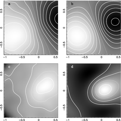
Figure 3: Comparison of the $\Omega=16\mbox{\,km\, s${}^{-1}$\, pc${}^{-1}$}$ model with kinematic maps. The axes in all panels are sky positions. (a) and (c) are maps of mean line–of–sight velocity, and velocity dispersion, respectively, taken from the “M8” data of Bacon et al. (2001); (b) and (d) are predictions of our model, including a constant bulge velocity dispersion of $150\mbox{\,km\, s${}^{-1}$}$, and smoothed with a Gaussian beam of FWHM $=0\aas@@fstack{\prime\prime}5$. In (a) and (b), the dotted line is the zero–velocity curve, and successive isocontours are in steps of $25\mbox{\,km\, s${}^{-1}$}$; positive (negative) velocities are in light (dark) shades. The dotted line in (c) and (d) corresponds to velocity dispersion of $200\mbox{\,km\, s${}^{-1}$}$, successive isocontours are in steps of $25\mbox{\,km\, s${}^{-1}$}$, and lighter shades indicate higher values.

We restored the Sérsic bulge profile, for comparisons with the photometry—see Figs. 2c and 2d, where the $\Omega=16\mbox{\,km\, s${}^{-1}$\, pc${}^{-1}$}\,$ model is compared with the photometry of Lauer et al. (1998). The locations of the peaks agree, although the model runs out of orbits near the edges. For kinematic comparisons, we further assumed that the velocity distribution of the bulge stars was Gaussian, with $\sigma_{v}=150\mbox{\,km\, s${}^{-1}$}\,$. Fig. 3 compares the model with the kinematic maps of Bacon et al. (2001). The need to smooth with a beam of $FWHM=0\aas@@fstack{\prime\prime}5$, rendered the absence of the outer orbits more acute. However, the zero velocity curves, as well as the orientation of the line joining the maximum and minimum velocities are in agreement (Figs. 3a and 3b); the dispersion maps are reasonably compatible in the region of the peak near P2 (Figs. 3c and 3d). As noted earlier, the best fits obtained for models with $\Omega=15,\,16,\,\mbox{and}\,17\mbox{\,km\, s${}^{-1}$\, pc${}^{-1}$}\,$. In Figs. 4a–4c, these are compared with the photometry of Lauer et al. (1998), and HST STIS kinematics from Bacon et al. (2001). Together, they should give some idea of the deviations from observations. The pattern speed has been variously estimated (Sambhus & Sridhar, 2000; Salow & Statler, 2001; Bacon et al., 2001) to lie between $3$ and $25\mbox{\,km\, s${}^{-1}$\, pc${}^{-1}$}\,$. Our present estimate, $\Omega\simeq 16\mbox{\,km\, s${}^{-1}$\, pc${}^{-1}$}\,$, is closest to Salow & Statler (2001) who, however, prefer to view the disk at the traditional inclination of $77{\degr}\,$.

We note here some limitations of our dynamical models. A basic assumption of our procedure was that the nuclear disk is razor–thin, and inclined at an angle of $(77^{\circ}-51.54^{\circ})\simeq 25^{\circ}$, with respect to the plane of the larger galactic disk of M31. We also ignored the gravitational force of the bulge stars on the nuclear disk, because the net effect of a spherically symmetric bulge would be to only modify the precession rates by a small amount. However, it is known (Kent, 1983, 1989) that the bulge of M31 is flattened, and this can be expected to modify the models in at least two ways. If the flattened bulge were treated as a fixed, external potential, the node of the nuclear disk will precess. The more serious effect arises from the dynamical friction of the bulge, acting on the stars composing the nuclear disk. The torque exerted by a flattened bulge, whose stars could have anisotropic distributions of velocities, could well decrease the inclination of the disk. However, we have not been able to estimate the response of the stellar disk, whose structure is so fundamentally determined by eccentric orbits locked in resonance.

The assumption that the nuclear disk is razor–thin is, of course, unrealistic. Tremaine (1995) estimates that two–body relaxation would thicken the disk significantly, within a Hubble time. Our choice of a razor–thin disk was made primarily for the recovery of a “unique” surface density distribution for the disk in its plane (Fig. 1c), from the observed surface photometry (Fig. 1a). This surface density was then used to calculate the disk self–gravity, possible orbit families for a range of pattern speeds, and then populating the orbit libraries appropriately using the RL algorithm. Consideration of a thick disk would have introduced an infinity of possible choices in the very first step of our procedure, and we wished to avoid it. It should, however, be stressed that an uninclined thick disk could well be compatible with observed photometry. This possibility should certainly be explored, perhaps by including kinematic data as additional constraints. A question that no one, presenting stellar dynamical models, can afford to ignore is whether the system is stable. There appears to be no better route to address this question, than N–body simulations. In this light we should regard the models presented in this paper as plausible guesses for further numerical explorations.

Figure 4: Further comparisons of models and observations. In (a), (b), and (c), the dashed–dot, solid, and dashed lines correspond to predictions of our model disks (including the bulge), with $\Omega=15,\,16,\,\mbox{and}\,17\mbox{\,km\, s${}^{-1}$\, pc${}^{-1}$}\,$. The dotted line in (a) is a cut along the P1–P2 line of the observed brightness, shown in Fig. 3a. In (b) and (c), the plotted data points are HST STIS observations (from Bacon et al. (2001)), of mean line–of–sight velocity and velocity dispersion, respectively, taken with a slit of width equal to $0\aas@@fstack{\prime\prime}1\,$, placed at PA of $39{\degr}\,$. The three lines represent similar “observations” of our models. In (d) we plot the LOSVD, observed with a Gaussian beam of FWHM $=0\aas@@fstack{\prime\prime}21$, for the $\Omega=16\mbox{\,km\, s${}^{-1}$\, pc${}^{-1}$}\,$ model (including bulge), centered on the MDO. The dashed line was computed after suppressing the retrograde orbits.

The “eccentricity” profiles of the loop orbits are given in Fig. 5a. The prograde loops have a characteristic non monotonic profile, whereas the retrograde loops have large eccentricites that increase monotonically with size, to the biggest orbits employed in our models. We note that the eccentricity profile of the prograde orbits is quite different from Salow & Statler (2001): in particular, there is no tendency for them to switch apoapses to the anti–P1 side of the MDO. The profiles of the apoapse angles (Fig. 5b) show no evidence for spirality; prograde/retrograde loops have their apoapses on the P1/anti–P1 side of the MDO. The disk mass is $1.4\times 10^{7}\mbox{\,M${}_{\sun}$}$, with $3.4\%$ on retrograde orbits; the central LOSVD in Fig. 4d indicate the positive and negative velocities at which the latter contribute. We have tried models with only prograde loops, but these gave consistently poor fits around P2.

Figure 5: Distribution of orbital eccentricities and apoapse angles, with orbit size. The “semi–major axis” is defined as the mean of the maximum and minimum radii ($r_{>}$ and $r_{<}$) of a parent loop; $\mbox{eccentricity}\equiv(r_{>}-r_{<})/(r_{>}+r_{<})\,$. In (a) and (b) the eccentricity and angle to apoapse, of parent loops, are plotted for a selection of prograde (filled circles) and retrograde (open circles) parent loop orbits. Prograde (retrograde) parents have apoapses on the P1 side (anti–P1 side) of the MDO.

Numerical simulations (Jacobs & Sellwood, 2001), and analytical study (Tremaine, 2001) indicate that nearly Keplerian disks (without counter–rotating streams) are neutrally stable to linear, $m\,=\,1$ perturbations. Hence it might appear unlikely that the lopsidedness could have grown spontaneously from an initially axisymmetric disk. Note, however, that in Bacon et al. (2001) there is reference to work, to be reported in the future by Combes and Emsellem, on an $m\,=\,1$ instability. Bacon et al. (2001) also suggest that a lopsided mode could have been excited by the passage of a massive object, such as a giant molecular cloud, or a globular cluster. They also report supportive simulations, where excited modes remained undamped for $7\times 10^{7}$ years, with almost constant pattern speed; this is certainly a plausible scenario.

Here we consider an alternative origin of the lopsidedness, based on the presence of the retrograde loops in our models, and recent work by Touma (2001) on a linear instability, in a softened–gravity version of Laplace–Lagrange theory of planetary motions. To the extent that softened–gravity mimics the velocity dispersions of stars (Miller, 1971; Erickson, 1974), this work suggests that even a few percent of mass in counter–rotating orbits could excite a linear $m\,=\,1$ overstability. In an axisymmetric nearly Keplerian disk, the apsides of prograde/retrograde orbits have negative/positive precession rates. A resonant response of the retrograde orbits (to a perturbation with positive $\Omega$) appears to excite large eccentricities. This compensates for their small mass fraction, allowing them to act so significantly, that the precession of apsides of the prograde loops is locked to that of the retrograde loops. We note that the large eccentricities of our retrograde loops (Fig. 5a), obtained directly from orbit integrations, are suggestive of this possibility. We speculate further that the overstability (as is common in other contexts) is arrested in growth by nonlinearity, and it settles into a nonlinear, neutral mode. The steadily rotating nuclear disk of M31 might well be in such a phase. Material on retrograde orbits could have been accreted by the infall of debris into the center of M31. One possibility is suggested by our estimate of the mass in retrograde orbits in our models, $\sim 5\times 10^{5}\mbox{\,M${}_{\sun}$}\,$. Tremaine, Ostriker, & Spitzer (1975) have argued that dynamical friction would cause globular clusters to spiral in toward galactic nuclei, and tidally disrupt. We could be witnessing the lopsided signature of such an event.