The stability of axisymmetric Taylor-Couette flow in hydromagnetics

Abstract

The linear marginal instability of an axisymmetric MHD Taylor-Couette flow of infinite vertical extension is considered. Only those vertical wave numbers are interesting for which the eigenvalue the (‘characteristic’) Reynolds number is minimal. For flows with a resting outer cylinder there is a well-known characteristic Reynolds number even without magnetic field but for certain (weak) magnetic fields there are solutions with smaller Reynolds numbers so that a characteristic minimum exists. We call those Reynolds numbers, the related wave number and the related Hartmann number as their critical values. The minimum only exists, however, for not too small magnetic Prandtl numbers (see Figs. 2 and 3 for a typical example). For small magnetic Prandtl numbers – or sufficiently small gaps – one only finds the typical magnetic-originated suppression of any instability.

More interesting are experiments where the outer cylinder rotates so fast that the Rayleigh criterion for hydrodynamic stability is fulfilled. We find that for given geometry and given magnetic Prandtl number now always a magnetic field amplitude exists where the characteristic Reynolds number is minimal. These critical values are computed for different magnetic Prandtl numbers and for three types of geometry (small, medium and wide gaps between the rotating cylinders). In all cases the Reynolds numbers are running with 1/Pm for small enough Pm, and the critical Reynolds numbers exceed values of 10⁶ for the magnetic Prandtl number of sodium (10^-5) or gallium (10^-6).

The container walls are considered as either electrically conducting or as isolators. Compared with the results for conducting walls, for small and medium size gaps between the cylinders i) the critical Reynolds number is smaller, ii) the critical Hartmann number is higher and iii) the Taylor vortices are longer in the vertical direction for isolating walls. For experiments with wide gaps the differences between both sets of boundary conditions become smaller and smaller.

I Introduction

The longstanding problem of the generation of turbulence in various hydrodynamically stable situations has found a solution in recent years with the so called ‘Balbus-Hawley instability’, in which the presence of a magnetic field has a destabilizing effect on a differentially rotating flow, provided that the angular velocity decreases outwards with the radius, [3]. This instability has been discovered decades ago [1], [2] for ideal Couette flow, but only after Balbus and Hawley it was recognized the importance of this magnetorotational instability (MRI) as the source of turbulence in the accretion discs with differential (Keplerian) rotation.

However, the MRI has never been observed in the laboratory ([4], [5], [6], [7]). Moreover, Chandrasekhar [2] already suggested the existence of MRI for ideal Taylor-Couette flow, but his results for non-ideal fluids for small gaps and within the small magnetic Prandtl number approximation demonstrated the absence of MRI for hydrodynamically stable flow. Recently, Goodman and Ji [9] claimed that this absence of MRI was due to the use of the small magnetic Prandtl number limit. The magnetic Prandtl number is really very small under laboratory conditions ($\sim 10^{-5}$ and smaller). Obviously, the understanding of this phenomenon is very important for possible future experiments, Taylor-Couette flow dynamo experiments included.

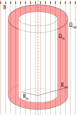
FIG. 1.: Cylinder geometry of the Taylor-Couette flow.

Here, the dependence of real Couette flow on magnetic Prandtl number and gap-width between rotating cylinders is investigated. The simple model of uniform density fluid contained between two vertically-infinite rotating cylinders is used with constant magnetic field parallel to the rotation axis. The unperturbed state is any stationary circular flows of an incompressible fluid. In the absence of viscosity, the class of such flows is very wide: indeed, if $\it\Omega$ denotes the angular velocity of rotation about the axis, then the equations of motion allow $\it\Omega$ to be an arbitrary function of the distance $R$ from the axis, provided the velocities in the radial and the axial directions are zero. For viscous flows, however, the class becomes very restricted: in fact, in the absence of any transverse pressure gradient, the most general form of $\it\Omega$ allowed is

$$\it\Omega(r)=a+b/{R}^{2},$$ (1)

where $a$ and $b$ are two constants related to the angular velocities $\it\Omega_{\rm in}$ and $\it\Omega_{\rm out}$ with which the inner and the outer cylinders are rotating. If $R_{\rm in}$ and $R_{\rm out}$ ($R_{\rm out}>R_{\rm in}$) are the radii of the two cylinders then

$$a=\it\Omega_{\rm in}{\hat{\mu}-{\hat{\eta}}^{2}\over 1-{\hat{\eta}}^{2}}\;\;{\rm and}\;\;b=\it\Omega_{\rm in}R_{\rm in}^{2}{(1-\hat{\mu})\over 1-{\hat{\eta}}^{2}},$$ (2)

with

$$\hat{\mu}=\it\Omega_{\rm out}/\it\Omega_{\rm in}\qquad{\rm and}\qquad\hat{\eta}=R_{\rm in}/R_{\rm out}.$$ (3)

After the Rayleigh stability criterion, $d(R^{2}\Omega)^{2}/dR>0$, rotation laws are hydrodynamically stable for $\hat{\mu}>\hat{\eta}^{2}$. Taylor-Couette flows with resting outer cylinders ($\hat{\mu}=0$) are thus never stable.

Here, in order to isolate the MRI we are mainly interested in flows with rotating outer cylinders so that the hydrodynamic-stability criterion $\hat{\mu}>\hat{\eta}^{2}$ is fulfilled. Our standard example is formed with $\hat{\eta}$=0.5 and $\hat{\mu}=0.33$.

II Basic equations

$R$, $\phi$, and $z$ are the cylindrical coordinates. A viscous electrically-conducting incompressible fluid between two rotating infinite cylinders in the presence of a uniform magnetic field parallel to the rotation axis leads to the basic solution $U_{R}=U_{z}=B_{R}=B_{\phi}=0$

$$B_{z}=B_{0}={\rm const.}\qquad U_{\phi}=aR+b/R,$$ (4)

with $U_{i}$ as the velocity and $B_{i}$ the magnetic field, $a$ and $b$ are given by (2). We are interested in the stability of this solution. The perturbed state of the flow may be described by

$$u_{R},\;U_{\phi}+u_{\phi},\;u_{z},\;b_{R},\;b_{\phi},\;B_{0}+b_{z},\;\delta P,$$ (5)

with $\delta P$ as the pressure perturbation.

Here only the linear stability problem with axisymmetric perturbations is considered. By analyzing the disturbances into normal modes the solutions of the linearized magnetohydrodynamical equations are of the form

$$u_{R}=u_{R}(R)e^{\omega t}\cos(kz),\ \ \ b_{R}=b_{R}(R)e^{\omega t}\sin(kz),$$ (6)

$$u_{\phi}=u_{\phi}(R)e^{\omega t}\cos(kz),\ \ \ \ b_{\phi}=b_{\phi}(R)e^{\omega t}\sin(kz),$$ (7)

$$u_{z}=u_{z}(R)e^{\omega t}\sin(kz),\ \ \ \ \ b_{z}=b_{z}(R)e^{\omega t}\cos(kz).$$ (8)

Stationary modes are always more critical than oscillatory ones, according to the results in [2] and [15]. So, only marginal stability will be considered ($\omega=0$). The derivation of the equations describing this situation is due to Chandrasekhar [2]; it should not to be repeated here. We only differ in the normalizations. Let $d=R_{\rm out}-R_{\rm in}$ be the gap between the cylinders. We use

$$H=(R_{\rm in}d)^{1/2}$$ (9)

as unit of length, the Alfvén velocity $V_{\rm A}=B_{0}/(\mu_{0}\rho)^{1/2}$ as unit of perturbed velocity and $B_{0}\cdot\mbox{Pm}^{1/2}$ as unit of perturbed magnetic field with the magnetic Prandtl number

$${\rm Pm}={\nu\over\eta},$$ (10)

$\nu$ is the kinematic viscosity, $\eta$ is the magnetic diffusivity. Note $H^{-1}$ as the unit of wave numbers.

Using the same symbols for normalized quantities as before the equations take the form

$$(DD_{*}-k^{2})^{2}u_{R}+k^{2}{\rm Ha}^{2}u_{R}-2k^{2}{\rm Re}{\it\Omega\over\it\Omega_{\rm in}}u_{\phi}=0,$$ (11)

$$(DD_{*}-k^{2})u_{\phi}+k{\rm Ha}b_{\phi}-{\rm Re}{1\over R}{d\over dR}\left(R^{2}{\it\Omega\over\it\Omega_{\rm in}}\right)u_{R}=0,$$ (12)

$$(DD_{*}-k^{2})b_{R}-k{\rm Ha}u_{R}=0,$$ (13)

$$(DD_{*}-k^{2})b_{\phi}-k{\rm Ha}u_{\phi}+{\rm Re}\mbox{Pm}R{d\over dR}\left({\it\Omega\over\it\Omega_{\rm in}}\right)b_{R}=0$$ (14)

(15)

with

$${\rm Ha}={BH\over\sqrt{\mu_{0}\rho\nu\eta}}\qquad{\rm Re}={\it\Omega_{\rm in}H^{2}\over\nu},$$ (16)

where ${\rm Ha}$ is the Hartmann number, ${\rm Re}$ is the Reynolds number of the inner rotation, $\rho$ is the density, $\mu_{0}$ is the magnetic constant. Chandrasekhar’s notations $D=d/dR$ and $D_{*}=d/dR+1/R$ are also used.

III Boundary conditions

An appropriate set of ten boundary conditions is needed to solve the system (15). The situation is more difficult than in the small-gap-small-Prandtl-number case where only eight boundary conditions are needed. Always no-slip conditions for the velocity on the walls are used, i.e.

$$u_{R}=0,\qquad u_{\phi}=0,\qquad{du_{R}\over dR}=0.$$ (17)

(see [2]). The magnetic boundary conditions depend on the electrical properties of the walls. The transverse currents and perpendicular component of magnetic field should vanish on conducting walls, hence

$${db_{\phi}\over dR}+{b_{\phi}\over R}=0,\qquad b_{R}=0.$$ (18)

The above boundary conditions (17) and (18) are valid for $R=R_{\rm in}$ and for $R=R_{\rm out}$.

The situation changes for isolating walls. The magnetic field must match the external magnetic field for nonconducting walls. The boundary conditions are different at $R=R_{\rm in}$ and $R=R_{\rm out}$ due to the different behaviour of the modified Bessel functions for $R\to 0$ and $R\to\infty$, i.e.

$$b_{\phi}=0,\;\;{\partial\over\partial R}(Rb_{R})=b_{R}{kRI_{0}(kR)\over I_{1}(kR)}\;\;{\rm for}\;\;R=R_{\rm in},$$ (19)

and

$$b_{\phi}=0,\;\;{\partial\over\partial R}(Rb_{R})=-b_{R}{kRK_{0}(kR)\over K_{1}(kR)}\;\;{\rm for}\;\;R=R_{\rm out},$$ (20)

(21)

where $I_{n}$ and $K_{n}$ are the modified Bessel functions (cf. [9]).

For a fixed Hartmann number, a fixed Prandtl number and a given vertical wave number we find the eigenvalues of the equation system. They are always minimal for a certain wave number which by itself defines the marginally unstable mode. The corresponding eigenvalue is the desired Reynolds number.

IV Results for conducting walls

We start with the results for containers with conducting walls and resting outer cylinders but with various gap sizes (medium, wide and small). In all these cases there are linear instabilities even without magnetic fields. The influence of the magnetic field is the question. If the resulting eigenvalue with magnetic field exceeds the eigenvalue without magnetic field then we have only the well-known effect of magnetic stabilization rather than magnetic destabilization. As we shall see, this is indeed the case for sufficiently small magnetic Prandtl numbers and/or for containers with a a small gap between the cylinders.

A Resting outer cylinder

In Fig. 2 a resting outer cylinder is considered ($\hat{\mu}$=0) for a medium-size gap of $\hat{\eta}$=0.5 and for Pm=1. As we know for vanishing magnetic field and for $\hat{\eta}$=0.5 the exact Reynolds number for this case is about 68 – well represented by the result for Ha=0 in Fig. 2. But for increasing magnetic field the Reynolds number is reduced so that figure the excitation of the Taylor vortices becomes easier than without magnetic field. The minimum Reynolds number Re_crit of about 63 for Pm=1 is reached for Ha${}_{\rm crit}\simeq$ 4…5. This magnetic induced subcritical excitation of Taylor vortices is due to the MRI. Always for a (say) critical Hartmann number the Reynolds numbers take a minimum which we shall call the critical Reynolds number. For even stronger magnetic fields – as it must be – the magnetic field starts to suppress the instability so that the Reynolds number starts to grow to infinity.

FIG. 2.: The stability line for Taylor-Couette flow with resting outer cylinder for $\hat{\eta}=0.5$ and Pm$=1$. The flow is unstable above the line. There is instability even without magnetic fields but its excitation is easier with magnetic fields with Ha $\simeq 4.5$. The line is marked with those wave numbers for which the eigenvalues are minimal.

In Fig. 3 the same container is considered but for the small magnetic Prandtl number of $10^{-5}$. The minimum characteristic for Pm=1 completely disappears, only suppression of the instability by the magnetic field can be observed.

FIG. 3.: The same as in Fig. 2 but for Pm=$10^{-5}$. The minimum characteristic for Pm=1 completely disappears.

A container with a small gap ($\hat{\eta}=0.95$) between the two cylinders is now under consideration (Figs. 4 and 5). Only magnetic suppression of the Taylor-Couette flow instability is observed in this case. This is the reason why Chandrasekhar did not find the MRI by his detailed numerical simulations for small gaps and very small magnetic Prandtl numbers. Fig. 5 are representing the small-gap-small-Prandtl approximation used by Chandrasekhar [2]. In order to find a minimum due to the MRI the magnetic Prandtl number must exceed 1, e.g. for Pm$=10$. The smaller the gap, the larger the Pm must be.

FIG. 4.: The stability line for the flow in a small gap ($\hat{\eta}$=0.95) with resting outer cylinder and for Pm$=1$. Note the disappearance of any minimum of the Reynolds number.

FIG. 5.: The same as in Fig. 4 but for Pm=$10^{-5}$.

In Fig. 6 the results for a container with a wide gap between the cylinders are given. Again we find the magnetic field only suppressing the instability for small magnetic Prandtl number. Obviously, the MRI does not work efficiently in the limit of small magnetic Prandtl numbers, i.e. for too low electrical conductivity Thus, if the electrical conductivity is so small as it is for sodium or gallium then the MRI cannot be observed by corresponding experiments with hydrodynamically unstable flows.

FIG. 6.: The stability line for the flow in a wide gap ($\hat{\eta}=0.25$) with resting outer cylinder ($\hat{\mu}=0$) for Pm=1 and Pm$=10^{-5}$.

B Rotating outer cylinder

Another situation holds if the outer cylinder may rotate so fast that the rotation law does not longer fulfill the Rayleigh criterion and a solution for Ha=0 cannot exist. Then the nonmagnetic eigenvalue along the vertical axis moves to infinity and we should always have a minimum. It is the basic situation in astrophysical applications such for accretion disks with a Kepler rotation law. Here in this paper the question is whether the critical Reynolds number and the critical Hartmann number can experimentally be realized. The Figs. 7…9 present the results for both various Hartmann numbers and magnetic Prandtl numbers for a medium-sized gap of $\hat{\eta}$=0.5.

FIG. 7.: The stability line for $\hat{\eta}=0.5$ and Pm=1. The outer cylinder rotates with 33% of the rotation rate of the inner cylinder so that after the Rayleigh criterion the hydrodynamic instability for Ha=0 disappears. The minimal Reynolds number is almost the same as in Fig. 2.

FIG. 8.: The same as in Fig. 7 but for Pm$=10^{-2}$.

FIG. 9.: The same as in Fig. 7 but for Pm=$10^{-5}$.

There are always minima of the characteristic Reynolds numbers for certain Hartmann numbers. The minima and the critical Hartmann numbers increase for decreasing magnetic Prandtl numbers. For $\hat{\eta}$=0.5 and $\hat{\mu}$=0.33 the critical Reynolds numbers together with the critical Hartmann numbers are plotted in Fig. 10.

For the small magnetic Prandtl numbers we find interesting and simple relations. With

$$C_{\Omega}={\rm Re}{\rm Pm}$$ (22)

and

$${\rm Ha}^{*}={\rm Ha}\sqrt{\rm Pm}$$ (23)

it follows

$$C_{\Omega}\simeq 20$$ (24)

and

$${\rm Ha}^{*}\simeq 3.5.$$ (25)

$C_{\Omega}$ is the magnetic Reynolds number, $C_{\Omega}=\it\Omega_{\rm in}H^{2}/\eta$ (or dynamo number) and Ha^∗ is the magnetic Hartmann number Ha${}^{*}=BH/\eta\sqrt{\mu_{0}\rho}$.

FIG. 10.: The main results for $\hat{\eta}=0.5$ and $\hat{\mu}=0.33$: The critical Reynolds numbers for given magnetic Prandtl numbers marked with those Hartmann numbers where the Reynolds number is minimal.

1 Wide gap

Let us now vary the size of the gap. In view of the experimental possibilities, we shall only work for conducting fluids with the magnetic Prandtl number of sodium, i.e. $10^{-5}$. In the present Section cylinders with a gap with $\hat{\eta}=0.25$ are discussed. The outer cylinder is either resting (Fig. 6) or it is rotating with a frequency fulfilling the Rayleigh criterion for stability (Fig. 11). In the first case, of course, there is a solution without magnetic field, i.e. for ${\rm Ha}=0$. The corresponding Reynolds number is 79. Note again that a minimum appears for Pm=1 which, however, does not survive the decrease of the magnetic Prandtl number to realistic small values.

The minimum always exists, however, for experiments with a rotating outer cylinder, e.g. for $\hat{\mu}=0.1$ (Fig. 11). The resulting critical Reynolds number is $1.15\cdot 10^{6}$ and the critical Hartmann number is about 500. Let us turn to first estimates. With $\nu=10^{-2}$ cm²/s the frequency $f$ of the inner cylinder is

$$f={1.6\cdot 10^{-5}{\rm Re}\over\hat{\eta}(1-\hat{\eta})}\left({10\ {\rm cm}\over R_{\rm out}}\right)^{2}\ \ {\rm Hz},$$ (26)

so that here

$$f={98\over\left(R_{\rm out}/10\ {\rm cm}\right)^{2}}\;{\rm Hz},$$ (27)

corresponding to the frequency of about 16 Hz for a container with an outer radius of 25 cm.

For the Hartmann number with the density for liquid sodium ($\rho\simeq 1\ {\rm g/cm}^{3}$) one finds

$${\rm Ha}=282\left({B\over{\rm Gauss}}\right)\left({R_{\rm out}\over 10\ {\rm cm}}\right)\sqrt{\hat{\eta}(1-\hat{\eta}){\rm Pm}},$$ (28)

hence for $\hat{\eta}=0.25$ and Pm=$10^{-5}$,

$${\rm Ha}=0.39\ \left({B\over{\rm Gauss}}\right)\left({R_{\rm out}\over 10\ {\rm cm}}\right)$$ (29)

results. For a container of (say) 25 cm a field of 500 Gauss yields thus a Hartmann number of 500. Note that this result has only a weak dependence on $\hat{\eta}$. It is thus not a problem to reach Hartmann numbers of order $10^{4}$ with the standard laboratory equipment.

We have to realize that Fig. 6 only displays suppression of the instability by the magnetic field for Pm=10^-5. There is no minimum of the Reynolds number due to the MRI instability. This effect is a consequence of the low magnetic Prandtl number. As it must, the instability disappears for ${\rm Ha}=0$ and $\hat{\eta}=0.25$ if $\hat{\mu}=0.1$ (Fig. 11). But here we find the instability again for a finite Hartmann number. For ${\rm Ha}\approx 500$ an instability occurs for a Reynolds number of about $10^{6}$. An experiment with a (say) Reynolds number of $1.5\cdot 10^{6}$ and an increasing magnetic field should yield the MRI instability between two known very sharp limits. The rotation frequency of the inner cylinder must fulfill the above relation (27), i.e. a container with an outer radius of 31 cm must rotate with a frequency of 10 Hz (see [11]).

FIG. 11.: Wide gap ($\hat{\eta}=0.25$): The same as in Fig. 6 (Pm$=10^{-5}$) but for a rotating outer cylinder with $\hat{\mu}=0.1$.

2 Small gap

For small gaps and resting outer cylinder there is no minimum due to MRI for magnetic Prandtl numbers equal or smaller than 1 (see Figs. 4 and 5) but it exists for e.g. Pm=10 (not shown). If the outer cylinder starts to rotate then the hydrodynamic instability goes to infinity and a minimum again appears due to the MRI (Fig. 12). However, the Reynolds numbers are much too high for a technical realization (inner rotation frequency is of order $10^{3}$ Hz). Obviously, MHD Taylor-Couette flows with too small gaps between the cylinders are not suitable for experimental work.

FIG. 12.: Small gap ($\hat{\eta}=0.95$): The same as in Fig. 5 but for a rotating outer cylinder with $\hat{\mu}=0.95$. Pm =10^-5, the critical Reynolds number is extremely high.

V Results for isolating walls

Containers with isolating walls must be considered. The (complicated) boundary conditions are then given by the relations (19) and (21). Surprisingly, the basic differences can already be demonstrated by the simplest model given in Fig. 13 for resting outer cylinder and Pm=1 (see Fig. 2 for comparison). Of course, the profiles start for Ha=0 with the same Reynolds number. The minimum, however, is deeper than in Fig. 2 and the corresponding Hartmann number is higher. Note that the vertical wavelength in the minimum is larger than in containers with conducting walls.

FIG. 13.: The same as in Fig. 2 but for isolating walls.

We shall check these findings in the following under restriction to a small magnetic Prandtl number (10^-5) and for rotating outer cylinders for small (Fig. 14), medium (Fig. 15) and wide (Fig. 16) gaps. The results must be compared with the results given in Figs. 9, 11 and 12 valid for conducting walls. For small and for medium gaps one finds indeed that i) the minimal Reynolds numbers are smaller, ii) the corresponding Hartmann number is higher and iii) vertical wave number is smaller (i.e. the cells of Taylor vortices are vertically more elongated) for the container with isolating walls. For wide gaps the critical Reynolds number is slightly higher for the container with nonconducting walls now but the vertical size of the cell is the same.

FIG. 14.: Small gap ($\hat{\eta}=0.95$): The same as in Fig. 12 but for the rotating outer cylinder ($\hat{\mu}=0.95$) embedded in vacuum. Pm=10^-5.

FIG. 15.: Medium-size gap ($\hat{\eta}=0.5$): The same as in Fig. 9 but for the rotating outer cylinder ($\hat{\mu}=0.33$) embedded in vacuum. Pm$=10^{-5}$.

FIG. 16.: Wide gap ($\hat{\eta}=0.25$): The same as in Fig. 11 but for the rotating outer cylinder ($\hat{\mu}=0.1$) embedded in vacuum. Pm=10^-5.

VI Vertical cell structure

The unstable Taylor-Couette flow forms Taylor vortices. With our normalizations the vertical extend $\delta z$ of a Taylor vortex is given by

$${\delta z\over R_{\rm out}-R_{\rm in}}={\pi\over k}\sqrt{{\hat{\eta}\over 1-\hat{\eta}}}.$$ (30)

The dimensionless vertical wavenumber $k$ is given in all the above figures.

In the case of hydrodynamically unstable flows we have $\delta z\simeq R_{\rm out}-R_{\rm in}$ for small magnetic field (Ha$\simeq 0$) independently on gap size and boundary conditions (see Figs. 2, 4, 6, 13). The cell has the same vertical extend as it has in radius (see [10]).

As all our figures demonstrate the influence of strong magnetic fields on turbulence consists on suppression and deformation. The deformation consists on a prolongation of the cell structure in vertical direction ([13]) so that $\delta z$ is expected to become larger and larger (the wave number becomes smaller and smaller) for increasing magnetic field. It is indeed true for Pm$\sim$1, but for smaller Pm the vertical cell size has a minimum for an intermediate value of the magnetic field (see Figs. 3, 5, 6).

The cell size is minimal for the critical Reynolds number for all calculated examples for hydrodynamically stable flow and conducting boundary (see e.g. Figs. 7, 11 and 12). This is not true, however, for containers with isolating walls for which the cell size grows with increasing magnetic field. For experiments with the critical Reynolds numbers the vertical cell size is generally 2…3 times larger than the radial one. The dependence of the vertical cell size on the magnetic Prandtl number is illustrated by the Fig. 17. The smaller the magnetic Prandtl number the bigger are the cells in vertical direction.

The influence of boundary conditions on the cell size disappears for wide gaps between the cylinders. For the small and medium gap, however, one finds the cells vertically more elongated for containers with isolating walls.

FIG. 17.: The same as in Fig. 10 but for the vertical wave number

VII Discussion

We have shown how the MRI works in Taylor-Couette flow experiments for fluids with high and low electrical conductivity and for conducting walls as well as for isolating ones. For given microscopic viscosity the electrical conductivity determines the magnetic Prandtl number which in the present paper is varied between 1 and $10^{-5}$.

For Pm=1 and large enough gap between the cylinders the MRI is realized by a clear minimum of the Reynolds number for certain (critical) magnetic fields with Hartmann numbers of order 10. The existence of the minimum does not strongly depend on the rotation rate of the outer cylinder – provided it rotates slower than the inner cylinder (Figs. 2, 7 and also 13).

There are drastic differences, however, for small magnetic Prandtl numbers or small gap between the cylinders. The minima completely disappear for resting outer cylinders (see Figs. 3, 4 and 5). But they survive for rotating outer cylinder (see Figs. 7….9 and also 15).

The coordinates of the minima strongly depend on the magnetic Prandtl number Pm. The critical Reynolds number scales as 1/Pm with the magnetic Prandtl number and the critical Hartmann number scales as $1/\sqrt{{\rm Pm}}$ for small Pm (see Fig. 10). We find the surprising result therefore that for sufficiently small magnetic Prandtl number both the magnetic Reynolds number $C_{\Omega}$ and the magnetic Hartmann number Ha^∗ (defined after (22) and (23)) depend only weakly on the magnetic Prandtl number.

Generally, the presented results tend to reduced critical Reynolds numbers for isolating rather than conducting walls. The power-law exponent (-1) which here results for an infinite cylinder is stronger than the value (-0.65) which has been found for a finite cylinder with pseudo-vacuum boundary conditions and a aspect ratio of 10 (cf. [14]).

¿From Eq. (26) with $\nu=10^{-2}$ cm²/s, $\hat{\eta}$=0.5 and Re$\simeq 1.8\cdot 10^{6}$ (see Fig. 10) for Pm$=10^{-5}$ follows

$$f={115\over\left(R_{\rm out}/10\ {\rm cm}\right)^{2}}\ {\rm Hz}$$ (31)

for the frequency of the inner cylinder. Hence, a container with an outer radius of 30 cm and an inner radius of 15 cm requires a rotation of about 10 Hz in order to exhibit the MRI for liquid sodium with its magnetic Prandtl number of 10^-5. After (25) the required magnetic field is about 900 Gauss.

The MRI is considered here only for axisymmetric disturbances. According to small gap small Pm results [16], the non-axisymmetric disturbances can be more unstable for small magnetic field. We are going to consider the influence of non-axisymmetric disturbances on MRI in a forthcoming paper.

REFERENCES

- [1] E. P. Velikhov, Sov. Phys. JETP 9, 995 (1959).
- [2] S. Chandrasekhar, Hydrodynamic and Hydromagnetic Stability (Clarendon, Oxford, 1961).
- [3] S. A. Balbus and J. F. Hawley, Astrophys. J. 376, 214 (1991).
- [4] R. J. Donnely and M. Ozima, Phys. Rev. Lett. 4, 497, (1960).
- [5] R. J. Donnely and M. Ozima, Proc. R. Soc. Lond. A 266, 272, (1962).
- [6] R. J. Donnely and D. R. Caldwell, J. Fluid. Mech. 19, 257, (1964).
- [7] A. Brahme, Physica Scripta, 2, 108, (1970).
- [8] H. Ji, J. Goodman and A. Kageyama, Month. Not. R. Astron. Soc. 325, 1, (2001).
- [9] J. Goodman and H. Ji, astro-ph/0104206, (2001).
- [10] E. L. Koschmieder, Bénard Cells and Taylor Vortices (Cambridge University Press, Cambridge, 1993).
- [11] D. P. Lathrop, J. Fineberg and H. L. Swinney, Phys. Rev. Lett. 68, 1515, (1992).
- [12] D. Richard and J.-P. Zahn, Astron. Astrophys. 347, 734, (1999).
- [13] G. Rüdiger, Astron. Nachr. 295, 275 (1974).
- [14] G. Rüdiger and Y. Zhang, Astron. Astrophys. (2001), in press
- [15] T. Chang and W. Sartory, Proc. Roy. Soc. A 301, 451, (1967).
- [16] C.-K. Chen and M. Chang, J. Fluid. Mech. 366, 135, (1998).