A FUSE SURVEY OF INTERSTELLAR MOLECULAR HYDROGEN IN THE SMALL AND LARGE MAGELLANIC CLOUDS

Abstract

We describe a moderate-resolution FUSE survey of H₂ along 70 sight lines to the Small and Large Magellanic Clouds, using hot stars as background sources. FUSE spectra of 67% of observed Magellanic Cloud sources (52% of LMC and 92% of SMC) exhibit absorption lines from the H₂ Lyman and Werner bands between 912 and 1120 Å. Our survey is sensitive to N(H₂) $\geq 10^{14}$ cm^-2; the highest column densities are log N(H₂) = 19.9 in the LMC and 20.6 in the SMC. We find reduced H₂ abundances in the Magellanic Clouds relative to the Milky Way, with average molecular fractions $\langle f_{\rm H2}\rangle=0.010^{+0.005}_{-0.002}$ for the SMC and $\langle f_{\rm H2}\rangle=0.012^{+0.006}_{-0.003}$ for the LMC, compared with $\langle f_{\rm H2}\rangle=0.095$ for the Galactic disk over a similar range of reddening. The dominant uncertainty in this measurement results from the systematic differences between 21 cm radio emission and Ly$\alpha$ in pencil-beam sight lines as measures of N(H I). These results imply that the diffuse H₂ masses of the LMC and SMC are $8\times 10^{6}$ $M_{\odot}$ and $2\times 10^{6}$ $M_{\odot}$, respectively, 2% and 0.5% of the H I masses derived from 21 cm emission measurements. The LMC and SMC abundance patterns can be reproduced in ensembles of model clouds with a reduced H₂ formation rate coefficient, $R\sim 3\times 10^{-18}$ cm³ s^-1, and incident radiation fields ranging from 10 - 100 times the Galactic mean value. We find that these high-radiation, low-formation-rate models can also explain the enhanced N(4)/N(2) and N(5)/N(3) rotational excitation ratios in the Clouds. We use H₂ column densities in low rotational states ($J$ = 0 and 1) to derive kinetic and/or rotational temperatures of diffuse interstellar gas, and find that the distribution of rotational temperatures is similar to Galactic gas, with $\langle T_{01}\rangle=82\pm 21$ K for clouds with N(H₂) $\geq$ 10^16.5 cm^-2. There is only a weak correlation between detected H₂ and far-infrared fluxes as determined by IRAS, perhaps due to differences in the survey techniques. We find that the surface density of H₂ probed by our pencil-beam sight lines is far lower than that predicted from the surface brightness of dust in IRAS maps. We discuss the implications of this work for theories of star formation in low-metallicity environments.

1. INTRODUCTION

Molecular hydrogen (H₂) must play a central role in our understanding of interstellar chemistry, but little is known about the distribution of diffuse H₂ in the interstellar medium (ISM) of the Galaxy. Major uncertainties remain about its formation, destruction, and recycling into dense clouds and stars (see the review by Shull & Beckwith 1982). Since the first detection of interstellar H₂ (Carruthers 1970) numerous studies (Copernicus, Savage et al. 1977, hereafter S77; ORFEUS, Richter 2000; FUSE, Shull et al. 2000) using ultraviolet absorption measurements of H₂ have created a general view of H₂ formation, destruction, and excitation in the diffuse ISM. However, we lack information about how the abundance of H₂ and its physical parameters depend on the environmental conditions of interstellar gas, such as the metallicity, dust content, and UV radiation field. The H₂ molecule has not been studied comprehensively in interstellar environments outside the Galactic disk. Varying metallicity and UV radiation may modify the molecular abundance, thereby affecting the interstellar chemistry that triggers the star formation process. In particular, the formation rate of H₂ in the diffuse ISM may depend on the composition and physical state of the gas and grains in unknown fashion.

Most of our knowledge of H₂ in the diffuse Galactic ISM comes from ultraviolet absorption measurements of the Lyman and Werner rotational-vibrational bands in the far ultraviolet (912 – 1120 Å). The Copernicus satellite mapped out the distribution and properties of H₂ along sight lines to stars confined to the local Galactic disk (Spitzer, Cochran, & Hirshfeld 1974; S77), and thus to a narrow range of gas properties. Despite this limitation, these studies uncovered important correlations between H₂ abundance and the environmental conditions (dust and gas). The basic volume limitation on studies of H₂ persisted until the advent of new instruments. The more sensitive but short-lived instruments, HUT (Gunderson, Clayton, & Green 1998) and ORFEUS (Dixon, Hurwitz, & Bowyer 1998; Ryu et al. 2000; Richter 2000), have extended the range of H₂ studies to selected distant sources in the Galaxy and the Magellanic Clouds, and the IMAPS spectrograph (Jenkins & Peimbert 1997; Jenkins et al. 2000) obtained high-resolution H₂ spectra of bright targets in diverse environments.

Molecular hydrogen is thought to form on interstellar dust grains when atoms are adsorbed on the grain surface, chemically bond there, and then are ejected from the grain surface (Hollenbach, Werner, & Salpeter 1971). Theoretical calculations, accounting for the probabilities of atom adsorption, and molecule formation and ejection, place the volume formation rate on grain surfaces at $n_{\rm H}n_{\rm HI}R$, where $R\approx 3\times 10^{-17}$ cm³ s^-1 in typical interstellar conditions, and where it is assumed that the total hydrogen density, $n_{H}$, is proportional to the number density of grains (Hollenbach & McKee 1979). Observations by Copernicus support this idea, with an inferred formation rate coefficient $R=(1-3)\times 10^{-17}$ cm³ s^-1 (Jura 1974). Correlations of H₂ and dust can provide a key test of this theory, but the narrow range of dust and gas properties in the Galactic disk accessible to Copernicus prohibited an exploration of the dependence of molecule formation on dust properties in a variety of environments. The lower-metallicity environments of the SMC and LMC (Welty et al. 1997; Welty et al. 1999) allow us to probe H₂ formation and destruction in physical and chemical environments different from the Galaxy. In particular, the 4- to 17- times lower dust-to-gas ratios in the Magellanic Clouds (Koornneef 1982; Fitzpatrick 1985) imply a smaller grain surface area per hydrogen atom and a correspondingly lower efficiency of H₂ formation.

The Magellanic Clouds are therefore a valuable nearby laboratory for studying H₂ in more distant, low-metallicity star forming regions and QSO absorption-line systems with high H I column density. Molecular hydrogen has been detected in three damped Ly$\alpha$ systems with N(H₂)/N(H I) in the range 10^-6 to 10^-4 (Ge & Bechtold 1999; Ge, Bechtold, & Kulkarni 2001; Petitjean, Srianand, & Ledoux 2000; Black, Chaffee, & Foltz 1987), and limits have been placed on molecular abundance in several other systems. Some of these systems are known to have low metallicity and/or high UV radiation intensity relative to the Galaxy. Detailed studies of H₂ in the nearby, spatially resolved Magellanic Clouds can serve as an important benchmark for comparison with these high-redshift systems.

Here, we describe the first survey results on H₂ in the ISM of the Magellanic Clouds obtained with the Far Ultraviolet Spectroscopic Explorer (FUSE) satellite. Initial FUSE results on H₂ in the Milky Way (Shull et al. 2000) suggest that diffuse H₂ is ubiquitous in the Galaxy. A large fraction of FUSE sight lines through the Galactic disk and halo exhibit absorption from the Lyman and Werner rotational-vibrational bands, showing that the Copernicus results on H₂ in the local regions of the disk extend, in principle, to more distant regions of the Galaxy. The sensitivity of the FUSE spectrograph allows the use of distant hot stars and extragalactic objects as background sources, opening up more distant regions of the Galaxy and beyond to study of the H₂ molecule. Our observations survey the H₂ abundance and properties in the low-metallicity regimes of the LMC and SMC, allowing us to model the formation and destruction rates of H₂, and the density and radiation field in the interstellar gas.

In § 2 we describe the observations and the data reduction and analysis schemes. In § 3 we survey the results on column densities, excitation, and other observed properties of the detected H₂, discuss correlations with other gas and dust properties along the sight lines, and compare these results to numerical cloud models. Section 4 discusses these results and summarizes the general conclusions of this survey. In this paper we assume a distance of 60 kpc to the SMC and 50 kpc to the LMC.

2. OBSERVATIONS AND ANALYSIS

2.1. FUSE Observations

The observations reported here comprise all the available LMC and SMC targets from FUSE Guaranteed Time Observations during Cycle 1 (up to October 2000). The FUSE mission and its instrumental capabilities are described by Moos et al. (2000) and Sahnow et al. (2000). The target stars were selected for campaigns to study O, B, and Wolf-Rayet stars (Program ID P117) and to examine hot gas in the Milky Way (MW) and Magellanic Clouds (P103). Seven of the SMC stars was chosen specifically for H₂ studies (P115). These observations present the first opportunity to study H₂ throughout the Magellanic Clouds in a comprehensive fashion. We include in the sample three SMC stars and one LMC star previously analyzed by Shull et al. (2000), the LMC star Sk -67 05, previously analyzed by Friedman et al. (2000) and the SMC star Sk 108, previously analyzed by Mallouris et al. (2001). An atlas of Magellanic Clouds stars observed with FUSE has been compiled by Danforth et al. (2001). We list the target stars, dataset names, and observational parameters in Tables 1 and 2. A summary of results appears in Tables 3 and 4, where we list detected column densities N(H₂), or upper limits, for the program stars. Tables 5 and 6 list individual rotational level column densities N(J) for the LMC and SMC, respectively, as derived from the curve-of-growth and/or line-profile fits (§ 2.2).

Figure 1.— The product $f\lambda^{2}$ for the Lyman 0-0 to 9-0 bands of H₂. Oscillator strengths and wavelengths are from Abgrall et al. (1993a,b). The best constraints on the H₂ curve of growth are provided by the relatively weak 0-0 and 1-0 bands. The right axis shows the 4 $\sigma$ column density sensitivity for the lines displayed, assuming that the limiting equivalent width of all lines is 30 mÅ (see Equation 1 and its discussion).

All observations were obtained in time-tag (TTAG) mode through the $30\arcsec\times 30\arcsec$ (LWRS) apertures. Most observations were broken into multiple exposures taken over consecutive orbital viewing periods (see Tables 1 and 2). The photon lists from these exposures were concatenated before being processed by the current version of the calibration pipeline software (calfuse v1.8.7). This program computes the shifts in the detected position of a photon required to correct for: (a) the motion of the satellite; (b) nodding motions of the diffraction gratings, which are induced by thermal variations on an orbital time scale; (c) small, thermally-induced drifts in the read-out electronics of the detector; and (d) fixed geometric distortions in the detector. Application of these shifts produces a two-dimensional, distortion-corrected image of a detector segment, from which a small, uniform background is subtracted. We extract one-dimensional spectra for the LiF and SiC channels recorded on each of the four detector segments. After correcting for detector dead time (which is small for count rates typical of targets in the Magellanic Clouds), we apply the most recent wavelength and effective-area calibrations to convert the detector count rate in pixel space to flux units as a function of heliocentric wavelength. Throughout these processing steps, we propagate 1 $\sigma$ uncertainties along with the data. No further modifications of the calfuse-processed data files are necessary for the H₂ analysis.

The FUSE detectors have very low dark count rates, and the overall level of light scattered to the detectors is low compared with the fluxes of our targets. Our targets range in specific flux from $F_{\lambda}=5\times 10^{-13}$ to $2\times 10^{-12}$ erg cm^-2 s^-1 Å^-1. The typical background count rate is the sum of dark counts and scattered light and corresponds to $<10^{-14}$ erg cm^-2 s^-1 Å^-1. The calfuse software performs a background subtraction, making the contribution of the background to the total error in continuum placement and equivalent widths negligible.

Figure 2.— Examples of FUSE spectra of SMC and LMC hot stars showing varying column densities of H₂. First panel: Sk -67 111 shows no detectable H₂ at LMC velocity, with N(H₂) $<5.0\times 10^{14}$ cm^-2. The Galactic H₂ lines are marked here for reference in the lower panels. Second panel: Sk -65 22, with N(H₂) = $7.6\times 10^{14}$ cm^-2. Third panel: Sk -69 246, with N(H₂) = $6.3\times 10^{19}$ cm^-2. Fourth panel: The SMC star Sk 82, with N(H₂) = $7.8\times 10^{15}$ cm^-2. The wavelength range is chosen to encompass the Lyman 4-0 band of H₂. The Lyman 5-0 P(4) line appears at left in the lower two panels.

Because FUSE contains no internal wavelength-calibration source, all data are calibrated using a wavelength solution derived from in-orbit observations of sources with well-studied interstellar components (Sahnow et al. 2000). This process leads to relative wavelength errors of 10 - 20 km s^-1 across the band, in addition to a wavelength zero point that varies between observations. Thus, we cannot rely completely on radial velocity measurements of interstellar absorption. In the analysis below, we derive relative velocities from H₂ lines and fix the zero point in each sight line by assuming that the Milky Way absorption lies at v_LSR = 0 km s^-1.

The resolution of the FUSE spectrograph across the band was $\lambda/\Delta\lambda\simeq$ 10,000-20,000 for these observations. Because many of these observations were acquired during testing and calibration phases of the FUSE mission, and because others were obtained late in 2000 after the instrument and its calibration had settled, the instrumental resolution and other parameters vary from target to target. However, since the results rely on measured equivalent widths and damping-profile fitting, our conclusions are not sensitive to the resolution and spectrophotometric calibration.

Figure 3.— Examples of the FUSE sample. The three stars shown are, from left to right: Sk -67 166 (also seen in Figure 4) and Sk -69 246 in the LMC and Sk 188 in the SMC. The J=0, 1, and 2 lines of the Lyman 4-0 band are shown, plotted in velocity space. They are chosen to show the velocity separations between Galactic and Magellanic H₂ and to bracket the range of detected H₂ column densities. The left line in each pair is the Milky Way component, the right line is the Magellanic Cloud component. The signal-to-noise ratios and resolution seen here are typical of our sample.

2.2. FUSE Data Analysis

In our analysis of H₂, we focus on the Lyman and Werner electronic transitions, with some 400 vibrational-rotational lines arising from the $J$ = 0 – 7 rotational states of the ground vibrational and electronic states of H₂. We search for $J\leq 7$, but lines above $J=4$ are difficult to detect in diffuse interstellar clouds, given the typical 4 $\sigma$ limiting equivalent width of 30 – 40 mÅ and the corresponding column density limit of $\rm N(H_{2})\simeq 10^{14}$ cm^-2. In this analysis we use oscillator strengths, wavelengths, and damping constants from Abgrall et al. (1993a,b). The line strengths $f\lambda^{2}$ for the R(0), R(1) and P(1) lines of the 0-0 to 9-0 Lyman bands appear in Figure 1. Starting at 0-0, the line strengths increase by roughly a factor of ten to 7-0 and then decline slowly as the upper vibrational level increases.

Figure 2 shows portions of FUSE spectra of four program stars, with a range of column densities N(H₂). We show the Lyman (4-0) vibrational band and label Milky Way and Magellanic lines. Absorption from gas in the Magellanic Clouds is easily distinguished by a large velocity separation in the range v = 200 - 300 km s^-1 for the LMC and 100 – 170 km s^-1 for the SMC. This paper is concerned with the Magellanic Cloud absorption only. Results on the detected Galactic gas in these sight lines will be presented later, together with other FUSE targets at high Galactic latitude.

Figure 3 shows the spectra of three selected stars, plotted in velocity space to show the relative positions and strengths of the H₂ lines of interest and the common blending between Galactic and Magellanic components. Figure 4 shows the entire FUSE spectrum of one LMC star, Sk -67 166. This figure illustrates the richness and complexity of FUSE data on H₂. We have identified the Lyman (red) and Werner (green) bands and the MW and LMC components. The LMC H₂ component has N(H₂) = $5.5\times 10^{15}$ cm^-2 and the MW component has N(H₂) = $5.0\times 10^{15}$ cm^-2.

We employ a complement of techniques when analyzing H₂ absorption lines. The final products of the analysis are measurements of the column densities in the individual rotational levels, N(J), from which we can infer the gas density, radiation field, and formation and destruction rates of H₂. For absorbers with $\rm N(H_{2})\lesssim 10^{18}$ cm^-2, we measure equivalent widths, $W_{\lambda}$, of all H₂ lines and produce a curve of growth (COG) to infer a Doppler $b$-parameter and N($J$). For high-column density absorbers with damping wings in the J = 0 and 1 lines, we fit the line profiles to derive N(0) and N(1), and we use a curve-of-growth technique to derive column densities for $J\geq 2$. However, there is no well-defined column density limit above which profile-fitting must be performed. Instead, it is used in any case for which no lines of J = 0 and 1 can be fitted with Gaussian line profiles, due to the presence of damping wings.

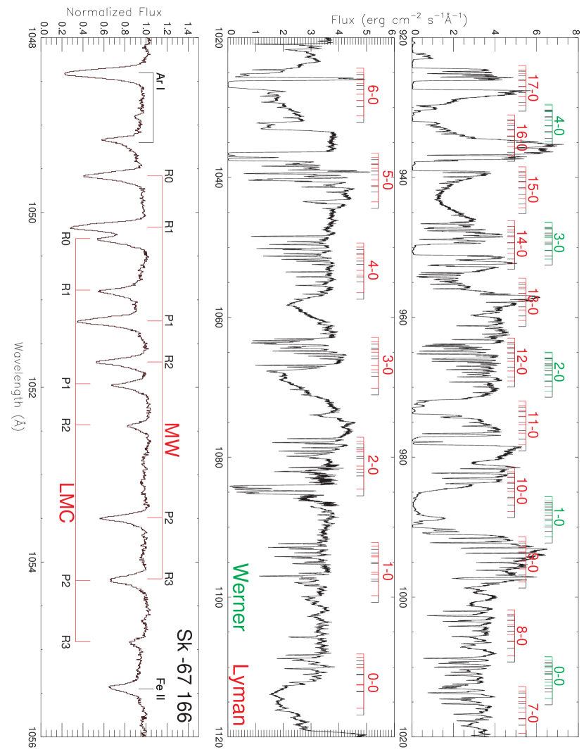
Figure 4.— Top two panels: FUSE spectrum of the LMC star Sk -67 166. This sight line has N(H₂) = $5.5\times 10^{15}$ cm^-2 in J = 0 – 3. The MW (black) and LMC (green and red) components are labeled within each band. Lower panel: The Lyman 4-0 band of H₂. LMC and MW lines are labeled. See the text for more discussion of this figure.

We are often forced to neglect H₂ lines in spectral regions near strong interstellar absorption or bright geocoronal emission. The H₂ Lyman (6-0) band is always lost in the strong damping wings of the interstellar Ly$\beta$ line (1025.7 Å), and the Lyman (5-0) band lies among the resonance absorption lines C II $\lambda$1036.3 and C II^∗ $\lambda$1037.0. We neglect these bands except when their $J\geq 2$ lines appear apart from the intervening absorption.

The key aspect of our analysis software is the rapid and consistent measurement of as many individual H₂ absorption lines as possible in each sight line. Variations in the data quality, line-of-sight structure, and spectral type of the source prevent the use of a uniform set of H₂ lines in the analysis. Thus, the process of measuring the numerous lines that enter the curve-of-growth fit cannot be automated completely. Our software requires the user to decide on a line-by-line basis which H₂ lines will be fitted.

First, model spectra of varying N(J) and $b$ are overlaid on the spectrum to obtain an estimate of the total column density N(H₂) and the radial velocities of the Galactic and Magellanic components. At this stage, detections are discriminated from non-detections and analyzed separately. We describe our analysis scheme for detections here and return to discuss non-detections below. Our software scans for H₂ lines from a list and queries the user at each line position. If the user decides the line is present and not severely compromised by blending, the line is fitted with a Gaussian profile, and its central wavelength ($\lambda_{0}$), equivalent width ($W_{\lambda}$), and full width at half maximum (FWHM) are stored in a table. The uncertainty in $W_{\lambda}$ is calculated, taking into account statistical errors in the data points and systematic uncertainty in the placement of the local continuum. A line scan is performed separately for each FUSE detector segment to avoid introducing systematic errors that may be associated with combining the overlapping segments into one dataset. Segment-by-segment analysis is common practice among FUSE investigators and we adopt it here. After each scan, lines that are blended or that were excluded from the scan for some other reason are fitted separately and placed in the table. There is one table for each of the four FUSE detector segments (1a,1b,2a,2b) and two channels (LiF and SiC), for a total of eight files.

At the conclusion of scanning, these tables contain the measurements for all the suitable H₂ lines in the spectrum, including multiple measurements for those lines that appear on more than one detector segment. There is a maximum of four measurements for each line. Prior to COG fitting, these tables are merged with the following scheme. The final $W_{\lambda}$ measurement for each line is the average of the individual measurements, weighted by the inverse squares of their individual uncertainties. The uncertainty in the final measurement is the maximum of these three quantities: (1) the quantity $(\sum\sigma_{i}^{2})^{-\frac{1}{2}}$, where the $\sigma_{i}$ are the individual uncertainties; (2) one-half the difference between the smallest and largest measurements (as a proxy for the standard deviation); or (3) 10% of the weighted mean itself. For most lines, (1) obtains the maximum value. However, for weak lines (2) is useful if duplicate measurements are widely separated and the formal standard deviation has little meaning. Finally, (3) is a conservative assumption that attempts to account for unquantified or unknown systematic errors in a uniform fashion.

After the individual line tables are combined, the software produces an automated fit to a curve of growth with a single Doppler $b$ parameter. This simple assumption is maintained throughout and is never clearly violated. Tests performed on high-quality data could not confirm the need for multi-valued $b$ increasing with J, an effect seen in Copernicus data (Spitzer et al. 1974) and attributed to unresolved components with different rotational excitation. We use a downhill-simplex method to minimize the reduced $\chi^{2}$ statistic, with column densities N(J) and $b$ as parameters. We typically obtain reduced $\chi^{2}$ in the range 0.5 - 2.0, with lower values for higher signal-to-noise data.

The simplex $\chi^{2}$-minimization technique is fully automated and well suited to deriving best-fit column densities and $b$, but it is inadequate for deriving realistic uncertainties in the measured parameters. The usual scheme of using the covariance matrix at the best-fit point to derive confidence intervals on the parameters is not appropriate in the highly nonlinear, multi-dimensional parameter space of the curve of growth. Typically, the quantity $\partial\chi^{2}/\partial p_{i}$ varies substantially with parameter $p_{i}$, such its value at the best-fit point does not accurately describe a midpoint between the critical $\chi^{2}$ values corresponding to the 1 $\sigma$ confidence interval. So, while we use a standard minimization technique for finding the best-fit column densities and $b$, we take a different approach to finding the maximum 1$\sigma$ variations in the parameters (the error bars in Tables 5 and 6).

In this multi-dimensional parameter space, the column densities N(J) and the Doppler $b$ parameter have somewhat different status, with the uncertainty in $b$ contributing most of the uncertainty in N(J). We first calculate the critical value, $\chi^{2}_{\rm crit}$, corresponding to the 1 $\sigma$ confidence interval. This quantity is given by the best-fit $\chi^{2}$ plus an offset $\Delta\chi^{2}$, which is distributed for $N$ parameters like $\chi^{2}$ for N degrees of freedom (Bevington & Robinson 1992). Over a range of $b$-values containing the best fit, the software produces a curve-of-growth fit over a succession of $b$ values, in 0.1 km s^-1 intervals. At each fixed $b$, the best fit is obtained by allowing N(J) to vary freely. If this best fit has $\chi^{2}<\chi^{2}_{\rm crit}$, then the column densities for different J are varied randomly to explore the parameter space in the immediate region of the best fit with fixed $b$. Randomly chosen column densities that satisfy the $\chi^{2}$ criterion are stored in a table for further analysis. This process is repeated over a range of fixed $b$ values, building a table of permitted parameters that satisfy the $\chi^{2}$ criterion. The quoted uncertainties in the published N(J) and $b$ represent the maximum variation among all the parameter sets that have $\chi^{2}<\chi^{2}_{\rm crit}$, and they represent the true 1 $\sigma$ joint confidence interval on the parameters.

In addition to its efficiency, this technique has the further benefit of providing realistic asymmetric error bars on the measurements. This technique is more efficient than a deterministic multi-dimensional grid, which requires many more COG evaluations if it is “square” in the parameters. By contrast, our technique does not vary the column densities if the best fit for a given $b$ is excluded. It requires approximately 10,000 COG evaluations for each sight line, far less than a deterministic grid with sufficient resolution to capture all the variations in the parameter space.

After COG fitting and exhaustive parameter space exploration, we have derived N(J), $b$, and uncertainties for each line of sight. However, for diffuse clouds with N(H₂) $\gtrsim 10^{18}$ cm^-2, it is better to derive N(0) and N(1) by fitting the wings of the damping profiles. For lines on the damping part of the COG, we combine the COG fitting technique described above with profile fitting. Model line profiles are produced with parameters N(J) and $b$ for each H₂ component in the spectrum, and convolved by a Gaussian instrumental line spread function. Typically, there are two components, corresponding to Galactic and Magellanic gas. Fitting is performed over the range of wavelength necessary to capture all the relevant lines and exclude difficult regions of the stellar continuum. The local continuum in the region of the fitted line profiles is described by a quadratic function. We also add atomic and ionic lines where necessary to improve the fit. Although H₂ lines with J $\geq$ 2 are included in the fitting, their final column densities are instead calculated using the COG fitting technique. Finally, we fit the Lyman bands separately on each FUSE detector segment and combine the measurements in a weighted average for final results. The uncertainties quoted in Tables 3 - 6 are the standard deviations of the multiple measurements (a more thorough discussion of this fitting is given by Rachford et al. 2001). We find remarkable consistency among the different Lyman bands and the different detector segments, giving us confidence that 10% uncertainty can be achieved routinely with this fitting method.

In a few cases, we derive very small uncertainties on N(0) and N(1). The most extreme case is Sk -69 246 for which the uncertainties are less than 10%. To test whether the data quality supports such small uncertainties, we have performed a Monte Carlo simulation of the effects of noise on the fits. We generate a noiseless profile based on the observed column densities, and then add a series of random noise vectors whose characteristics match the observed noise in the object spectra. For Sk -69 246 we generated 10 noisy synthetic spectra and performed profile fits. The standard deviations of the values of N(0) and N(1) were 0.01 dex, smaller than the reported uncertainties. This result supports the claim that the segment-to-segment variations in the fitted values dominate the total uncertainty.

In our line analysis, COG fitting, and profile fitting, we have paid careful attention to statistical and systematic uncertainties in deriving H₂ column densities and Doppler parameters. The major source of uncertainty in the column densities derived from COG fitting is the often weak constraint on the Doppler $b$ parameter. Generally, lines from a given rotational level with a wide range of line strengths ($f\lambda$, the oscillator strength times the rest wavelength in Å) are necessary to adequately constrain $b$ for a given sight line (see Figure 1). In practice, the best constraints are provided by the relatively weak Lyman 1-0 and 0-0 bands. If lines with both high and low $f\lambda$ are available, or for lines on the linear portion of the COG, the logarithmic errors in the column densities can approach 0.10 dex, and vary with the signal-to-noise ratio. If the available lines for a given J-level are spaced narrowly in $f\lambda$, the error in this column density will be determined largely by the permissible range in $b$. In this case, solutions for the N(J) are coupled together by the $b$ value; lowering or raising $b$ will move all the N(J) up or down together, respectively. Large uncertainties in $b$ can also cause very asymmetric error bars on the column densities. If the best-fit column density for a given $b$ lies near the best-fit N(J) for the extreme end of the $b$ range, then the N(J) may take on a large uncertainty in the other direction, corresponding to the other extreme of $b$. All these systematic variations make the ratios in the column densities (seen below in § 3) less uncertain than the individual column densities themselves.

A further systematic uncertainty is due to the unknown component structure of the H₂ clouds. At the 15 - 30 km s^-1 resolution of FUSE, we generally cannot resolve the fine-scale structure of complicated interstellar components observed in atomic lines with higher resolution (e.g., by Welty et al. 1997, 1999). Our analysis assumes that all the H₂ resides in one component, and that absorption from all rotational levels can be described by a single Doppler $b$. Snow et al. (2000) and Rachford et al. (2001) used the observed Na I component structure along Galactic translucent-cloud sight lines to construct a multicomponent curve of growth. Here, the stronger absorption makes it more likely that H₂ is contained in more than one component. They found that, while the measured column densities N(J) were sensitive to the component structure, the differences in N(J) for lines on the Doppler (flat) portion of the COG were small compared to the uncertainties associated with the flat COG. Thus, we assume single-component structure and leave more detailed analysis for future examination of individual sight lines from our survey.

The sight lines in which H₂ is not detected receive a separate analysis. If there is no visible evidence of the strong Lyman 7-0 R(0) and R(1) lines, we place upper limits on the equivalent widths of these lines and convert these limits to column density limits assuming a linear curve of growth. We use the following expression for the (4 $\sigma$) limiting equivalent width of an unresolved line at wavelength $\lambda_{0}$:

$$W_{\lambda}=\frac{4\lambda_{0}}{(\lambda/\Delta\lambda)\,(S/N)},$$ (1)

where $\lambda/\Delta\lambda$ is the spectral resolution, and S/N refers to the signal-to-noise ratio per resolution element in the 1-2 Å region surrounding the expected line position. By contrast, in Tables 1 and 2 we list the S/N ratio per pixel to provide a means of comparing datasets in a resolution-independent fashion. Because the resolution of FUSE varies across the band and even between observations, we conservatively assume $\lambda/\Delta\lambda$ = 10,000 for all upper limits. The N(0) and N(1) limits in Tables 5 and 6 are imposed with the strongest J = 0 and J = 1 Lyman lines, 7-0 R(0) and 7-0 R(1). For a linear COG, these lines have equivalent widths $W_{\lambda}=(26.8$ mÅ) (N(0) / 10¹⁴ cm^-2) and $W_{\lambda}=(18.7$ mÅ) (N(1) / 10¹⁴ cm^-2), respectively. The entries in Tables 3 and 4 show a limit on the sum of the two individual lines. Most of the upper limits lie just below the lowest detections of H₂.

In summary, we describe the results and uncertainties that appear in Tables 5 and 6. We list the final column density and uncertainty results for all our program stars. These column densities were derived from the COG or profile-fitting routines described above. The uncertainties were calculated from either COG parameter-space searches or band-to-band and segment-to-segment variations in the profile fits, again as described above. The 4 $\sigma$ upper limits are derived according to Equation (1) from individual signal-to-noise ratios of the data in the region of of the Lyman 7-0 R(0) and R(1) lines. For these limits we assume an effective resolution $R$ = 10,000. For low-column density sight lines where no constraint on the Doppler $b$ parameter is provided, we assume that the lines fall on the linear portion of the curve of growth and label these cases accordingly. These tables form the fundamental database for all subsequent analysis.

2.3. Notes on Individual Sight Lines

The LMC targets Sk -69 243 (R136) and MK 42 lie at the center of the 30 Doradus H II region, and Sk -69 246 lies in an isolated field 4^′ to the north. The Sk -69 246 spectrum shows no evidence of unusual properties. The other two datasets, however, show line profiles much broader than the expected FUSE line spread function in both the LMC and Galactic absorption lines due to crowding among the 70+ hot stars in the inner 30^′′ of the cluster. Because the blurring mimics a low-resolution spectrograph, we can only be sure that there is H₂ at LMC velocities in these sight lines, with N(H₂) $\simeq 10^{19}$ cm^-2. The crowded fields and line broadening preclude a detailed analysis of the column densities. We include these stars in the H₂ detection statistics (Tables 1 and 3) but exclude them from the LMC column density sample (Table 5).

The sight lines to NGC 346 (3, 4 and 6) lie within a 50^′′ circle on the sky in the SMC. As seen in Tables 4 and 6, their column densities and Doppler $b$ parameters are statistically indistinguishable, suggesting that these closely spaced sight lines probe the same interstellar cloud. In the abundance and excitation distributions and tests performed below, we use the mean column density in each level and the mean $b$ to stand in for these three sight lines.

Mallouris et al. (2001) reported tentative detections of J = 1 and J = 3 lines in towards the SMC star Sk 108. Our survey imposes formal 4 $\sigma$ limits on the equivalent widths of undetected H₂ lines. According to this criterion, these lines are not significant, and we place an upper limit on N(H₂) for Sk 108 that is larger than the value they report.

For closely paired sight lines we can use the observed H₂ excitation to estimate the sizes of diffuse interstellar clouds. The sight lines to HD 5980 and AV 232 are separated by 58^′′ on the sky, and lie $\simeq$ 17 pc apart at the distance of the SMC. Shull et al. (2000) reported different rotational excitation N(J) in these two sight lines, indicating that they may probe different molecular gas. The Galactic components in these sight lines show similar column densities and kinetic temperatures, and are likely to arise from the same cloud. However, the SMC H₂ components on these two sight lines show distinct differences in rotational excitation. Measurement of H₂ excitation and abundance in multiply-intersected absorbers will allow us to constrain the sizes and structure of diffuse interstellar clouds.

2.4. Ancillary Data

To fully exploit the FUSE data on H₂, we require additional information about the dust and gas along the sight lines. The most important of the supplemental data is the atomic hydrogen column density along each sight line. To obtain N(H I) for our entire sample, we use 21 cm radio emission and apply a correction to account for known systematic errors.

We obtain H I column densities from the recent Parkes and Australia Telescope Compact Array maps (SMC, Stanimirovic et al. 1999; LMC, Staveley-Smith et al. 2001) and then apply a correction, discussed below. These maps were created with $60^{\prime\prime}$ (LMC) and $98^{\prime\prime}$ (SMC) beams and were provided to us in fully calibrated, machine-readable form (L. Staveley-Smith, personal communication). To obtain the N(H I) for the FUSE sight lines, we select the four beam positions that surround each star and perform a bilinear interpolation. Using N(H I) from 21 cm emission may be subject to systematic uncertainties associated with dilution in the 1^′ beam if the interstellar gas is highly clumped on smaller scales or if there is additional emission behind the stars. Available UV absorption measurements provide a valuable check on these measurements.

Attempts to derive N(H I) from the Ly$\beta$ lines in the FUSE band generally fail, owing to the severe blending between the Galactic and SMC/LMC components, geocoronal O I emission, and the presence of the H₂ absorption. The higher Lyman series is present in the FUSE band but is severely compromised by the dense forest of H₂ and atomic lines below 1000 Å. Data on H I Ly$\alpha$ are available for roughly two-thirds of our sample, but we find that reliable determinations of N(H I) from a combination of Ly$\alpha$ and Ly$\beta$ profile fitting is impractical in all but the best cases. The largest uncertainties are in the placement of the stellar continuum near these lines and in the close velocity spacing of the Galactic and Magellanic components (100 - 300 km s^-1). While determinations could be made for roughly 30% of the targets with high-resolution, high-S/N data (from HST/FOS, GHRS, and particularly STIS) and simple continuum structure, we could not achieve this goal for the entire sample. We performed simple fits to the Ly$\alpha$ profiles to estimate N(H I) for the one-third of the sample where the profile is not severely compromised. In these trials, we found that the constraints on N(H I) range from 0.3 to 1.0 times the 21 cm value, with a mean of 0.56 for both Clouds. We have not attempted to remove contaminating absorption and complicated features in the stellar continuum, which are present even in these best cases. Thus, fitting the Ly$\alpha$ profile is itself uncertain, and generally establishes an upper limit. The lower limit is more difficult to determine because the Magellanic component can be reduced and the Galactic component increased to compensate. However, it appears that for 25 sight lines, the upper limit derived from Ly$\alpha$ is, on average, half its value from 21 cm emission. This result suggests that we should adjust our H I column densities to account for this systematic error.

We are reluctant to apply a uniform factor of 0.5 correction to the entire FUSE sample, because the subsample may have internal biases. For example, the stars with HST data may be located preferentially on the front sides of the Clouds. As a compromise between uniformity and uncertainty, we reduce the 21 cm N(H I) by a factor 0.75. We then impose a large uncertainty on N(H I) to account for this systematic error. For the final column density, we adopt N(H I) = ($0.75^{+0.25}_{-0.25})\,\,\times$ N(21 cm). This scheme captures the uncertainty in the column density and can be applied to the entire sample. Both extremes, at the high end from 21 cm data and at the low end from our HST estimates, are included in the error bars. The final uncertainty in the molecular fraction is dominated by the uncertainty in N(H I).

The color excess, E(B-V), is an important measure of the dust abundance towards the target stars. The color excesses were obtained using two methods: (1) the observed B-V color and an adopted intrinsic (B-V)₀ scale (Fitzgerald 1970 and Schmidt-Kaler 1982, with -0.31 or -0.32 adopted for early giants and supergiants), and (2) the observed UV spectrophotometry (IUE) plus B and V together with model atmospheres to fit the spectral energy distribution. In practice, we take the mean of the two methods to minimize any external uncertainties. Because intrinsic colors for Wolf-Rayet (WR) stars vary dramatically, model atmospheres together with UV and optical spectrophotometry are necessary to derive E(B-V). We estimate the final uncertainty in these values to be $\leq$ 0.02 mag. A further uncertainty is the contribution of foreground dust to the total sight line reddening. We derive the corrected color excess, E^′(B-V), by subtracting from the measured color excess a foreground E(B-V) = 0.075 for the LMC and 0.037 for the SMC. These average values were obtained by the COBE/DIRBE project by averaging the dust emission in annuli surrounding the Clouds (Schlegel, Finkbeiner, & Davis 1998). In § 3 we describe a test of these averages with the observed gas-to-dust ratio.

We use the Copernicus survey of Savage et al. (1977) to compare the similarities and differences between the FUSE sample and H₂ in the disk of the Galaxy. The sample of 109 stars obtained by S77 (their Table 1) was culled for the 51 stars with measured N(H I), either a measurement or limit on H₂, and E(B-V) $\leq 0.20$. The 17 upper limits in this sample are included in certain tests depending on the context of the comparison. In addition, we compiled column densities for $J\geq 2$ for 31 of these stars from Spitzer, Cochran, & Hirshfeld (1974). These column densities are compared to the rotational excitation of the LMC and SMC gas in § 3.

2.5. Sample Selection and Bias

Most of the FUSE sample of LMC and SMC stars was not chosen specifically for the H₂ survey. Most of the sample is drawn from three large FUSE team programs devoted to stellar and interstellar research. The stellar wind (Program P117) targets were chosen to occupy a range of spectral types. The allotted time for each observation was 4 ksec, so this is essentially a flux-limited sample. In practice, this criterion selects against stars with substantial extinction, which would be favored in a sample chosen to study H₂. The stars in Program P103, the FUSE study of hot gas in the Magellanic Clouds, were chosen based on the availability of supporting observations and to probe the supershells and bubbles in the ISM of the LMC. In effect, this program selected against denser regions and high extinction in favor of regions where cavities of hot gas are expected. In the SMC, seven stars were chosen specifically for H₂ studies (Program P115). All others were drawn from the hot star or hot gas programs. However, from the point of view of this survey, the stars are located randomly across the LMC and SMC, but probably preferentially situated on the Milky Way side of the dense absorbing regions in the two galaxies.

In addition to these selection biases, there is the additional problem that flux-limited or extinction-limited surveys favor targets on the foreground face of the LMC and SMC. This bias complicates the use of H I column densities derived from emission measurements. The 21 cm emission beam samples all the gas, including some that lies behind the target star but does not appear in absorption along the FUSE pencil-beam sight lines. In this case, the measured gas-to-dust ratio, or N(H I) / E^′(B-V), will be enhanced over the average ratio determined using H I Lyman series absorption to derive N(H I). Figure 5 compares the corrected color excesses for the program stars with their H I column densities from 21 cm emission, corrected as in § 2.4. The values of N(H I) / E^′(B-V) range from $10^{22}-10^{23}$ cm^-2 mag^-1 for the LMC stars, with a general trend towards decreasing values of the ratio with higher E^′(B-V). There is a similar trend in the SMC, with N(H I) / E^′(B-V) = $10^{22.5}-10^{23.5}$ cm^-2 mag^-1. We plot the average value of this ratio for targets in the disk of the Milky Way as determined from IUE measurements by Shull & van Steenberg (1985), and the average values for the LMC (Koornneef 1982) and the SMC (Fitzpatrick 1985). Our target stars lie well above the Galactic average, but are consistent with the LMC and SMC values. Because E^′(B-V) appears in both axes of this plot, the error bars on the points should run diagonally from the upper left to the lower right of each point. This fact probably explains the trend seen in the points, with lower E(B-V) lying above the average and higher E(B-V) below. We conclude that, while the location of the stars in the gas layers of the LMC and SMC may account for some of the scatter in the molecular fraction results, there is no large systematic increase in N(H I) and no corresponding systematic change in quantities derived from it. The observed trends suggest that our adopted correction to the 21 cm H I columns is reasonable. Had we adopted a larger correction to the 21 cm columns, the points that lie below the average gas-to-dust ratios would be far more discrepant. For further discussions of uncertainty in N(H I), see § 2.4.

3. SURVEY RESULTS AND ANALYSIS

3.1. General Results

A summary of results appears in Tables 3 and 4, where we list detected column densities N(H₂), or upper limits, for the program stars. Tables 5 and 6 list individual rotational level column densities N(J) for the LMC and SMC, respectively, as derived from the curve-of-growth and/or line-profile fits (§ 2).

The immediate, striking result of this survey, apparent from Tables 3-6, is the lower frequency of H₂ detection in the LMC compared with the SMC. Shull et al. (2000) reported seven sight lines through the Galactic disk and halo, only one of which did not show detectable H₂ (PKS 2155-304). The detection rate in the initial FUSE sample of extragalactic targets exceeds 90%. However, the total rate of detection in the LMC is 23 detections in 44 sight lines, for a 52% success rate. In the SMC, the detection rate is 24 of 26, or 92%. This difference appears to be related to the patchy structure of the LMC ISM, which contains many identified H I superbubbles blown out by OB associations and supernova remnants (Kim et al. 1999). By comparison, the ISM of the SMC is more quiescent and less patchy (see § 4-5 for further discussion).

3.2. H₂ Abundance

The lower abundance of H₂ in the low-metallicity gas of the LMC and SMC is a key result of this survey. The molecular hydrogen abundance is sensitive to the formation/destruction equilibrium of H₂ in diffuse gas, where far-ultraviolet (FUV) radiation competes with formation on dust grains to determine the relative abundance of H₂. The size of the sample allows us to apply statistical tests of H₂ abundance in the LMC and SMC and compare it to H I, dust properties, and diagnostics of the UV radiation field. The reduced molecular fraction may indicate less efficient formation of H₂ molecules on interstellar dust grains or enhanced H₂ photo-dissociation by an intense FUV radiation field, or a combination of these two effects. In this section, we use simple analytic expressions and numerical models to assess the effects of varying environmental conditions on the H₂ formation/destruction equilibrium.

To assess the total abundance of H₂, we define the quantity $f_{\rm H2}$ = 2N(H₂) / [N(H I) + 2N(H₂)], which expresses the fraction of hydrogen nuclei bound into H₂. The molecular fractions for our sight lines appear in Figure 6, correlated with the corrected color excesses of the target stars. In Figure 7 we compare the S77 sample of Galactic disk stars with the LMC and SMC targets. The key difference between the samples is the presence of several LMC and SMC sight lines with $f_{\rm H2}$ $\geq 10^{-4}$ at low E^′(B-V). In the Clouds we find a wide range of molecular fractions at low reddening, E^′(B-V) $\leq 0.08$. In the LMC there is a noticeable gap near $\log$ $f_{\rm H2}$ $=-4$, which does not appear in the SMC. The most striking pattern in these plots is the large number of sight lines to the LMC that show no detectable H₂. S77 found low values of $f_{\rm H2}$ at low E(B-V) and a transition from low to high values ($f_{\rm H2}$ $\sim$ 0.1) at a color excess E(B-V) = 0.08. This pattern is not readily discernible in the samples.

Our results reverse prior indications that the average molecular fraction in the LMC is not reduced relative to the Galaxy. Using HUT, Gunderson et al. (1998) measured N(H₂) $\simeq$ 10²⁰ cm^-2 for two LMC stars, Sk -66 19 and Sk -69 270, that do not appear in our sample. These sight lines have $f_{\rm H2}$ = 0.04, similar to the highest-$f_{\rm H2}$ points in the FUSE sample. They concluded that, in the low-metallicity LMC, N(H₂)/E(B-V) did not differ from the average Galactic value, despite large differences in N(H I)/E(B-V). With the larger FUSE sample, we find a substantial reduction in $f_{\rm H2}$ in the LMC. With ORFEUS data on three LMC stars, Richter (2000) found that, although N(H₂) relative to E^′(B-V) in the Clouds might be similar to the Galactic values, the N(H₂)/N(H I) ratio was lower than the Galactic average. The larger FUSE sample confirms this result.

To quantitatively compare the distributions of $f_{\rm H2}$ for the Galaxy and Magellanic Clouds, we performed Kolmogorov-Smirnov (KS) tests on the samples. The two-sided KS test finds a 0.224 probability that the S77 and SMC samples are drawn from the same parent distribution, and a $<$0.001 probability for the S77 and LMC samples. Compared to each other, the SMC and LMC samples give a 0.121 probability of being drawn from the same distribution. This difference reflects the very different detection rates in the Clouds, but they suggest that the reduced $f_{\rm H2}$ in both the LMC and SMC is significant.

For a quantitative comparison of the Galactic disk and LMC molecular fractions, we define the average column-density weighted molecular fraction $\langle f\rangle$ to be:

$$\langle f\rangle=\sum\rm 2N(H_{2})/\sum[N(\rm H~{}I)+2N(\rm H_{2})].$$ (2)

In evaluating the average molecular fractions, we include the FUSE upper limits as measurements, so that $\langle f\rangle$ from FUSE is also an upper limit. For the LMC, we find $\langle f\rangle=0.012$ for stars with E^′(B-V) = 0.00 - 0.20. For the SMC, we find $\langle f\rangle=0.010$ for stars with E^′(B-V) = 0.00 - 0.12. For the Galactic comparison sample, we find $\langle f\rangle=0.039$ for stars with E(B-V) = 0.00 - 0.12, for comparison with the SMC. For Galactic stars with E(B-V) = 0.00 - 0.20, we find $\langle f\rangle=0.095$, for comparison with the LMC. If we exclude the upper limits in Tables 5 and 6 from the sample, we find $\langle f\rangle=0.010$ for the SMC and $\langle f\rangle=0.021$ for the LMC, due to the large large number of non-detections there.

Figure 8 shows the individual and cumulative molecular fractions correlated with the total H content, N(H) = N(H I) + 2N(H₂). The S77 sample shows a clear break near log N(H) = 20.7, above which all clouds have molecular fraction $f_{\rm H2}$ $\sim 0.1$. This break is usually identified as the point at which the cloud achieves complete self-shielding from interstellar radiation (S77). The LMC and SMC sight lines show no such clear transition, even at the higher N(H) they probe. As we show below, the LMC and SMC show evidence of reduced formation rate of H₂ on dust grains and of enhanced photo-dissociating radiation relative to the Galaxy. In this case, we expect to see a transition from small $f_{\rm H2}$ with large scatter to a tighter band of high $f_{\rm H2}$, but at a higher total H column density than in the Galactic disk. The FUSE samples require that such a transition occurs at $\log N(H)\geq 21.3$ in the LMC and $\log N(H)\geq 22$ in the SMC. Planned observations of several LMC and SMC stars with E^′(B-V) $\geq$ 0.20 will address this point in the future.

The lower observed $\langle f\rangle$ is evidence for lower molecular abundance in the LMC and SMC. However, there is a potential systematic effect that we must reemphasize. The S77 survey used column densities, N(H I) and N(H₂), determined from the same Copernicus spectra. This technique does not suffer the systematic uncertainty of comparing measurements of N(H I) from radio emission measurements with a large beam and N(H₂) determined from pencil-beam sight lines. Thus, relative to the S77 measurements, we may underestimate the molecular fraction due to the systematic overestimate of the H I column determined from 21 cm emission if a substantial fraction of the H I seen in emission lies behind the target star or if clumping is significant below 1^′ scales. However, because the average dust-to-gas ratio for our targets scatter around the average values found for the LMC and SMC, this problem is unlikely to exceed the generous error budget assigned to N(H I). (See the discussion of these issues in § 2).

A simple model of H₂ in an interstellar cloud (Jura 1975a,b) can be expressed as an equilibrium between the formation of H₂ with a rate coefficient $R$ (in cm³ s^-1) and the photodestruction of H₂ with rate $D$ (in s^-1):

$$Rn_{HI}n_{HI}=Dn(H_{2})\simeq f_{\rm diss}\sum_{J}\beta(J)n(H_{2},J),$$ (3)

where $\beta(J)$ is the photoabsorption rate from rotational level J and $n_{H}=n(H~{}I)+2n(\rm H_{2})$. The coefficient $f_{\rm diss}$ corresponds to the fraction of photoabsorptions that decay to the dissociating continuum and varies from 0.10 to 0.15 depending on the shape of the UV radiation spectrum. Molecules are destroyed by photoabsorption in the Lyman and Werner bands, followed by radiative decay to the vibrational continuum of the ground electronic state. The formation of H₂ is believed to occur on the surfaces of dust grains, but may also occur in the gas phase at a lower rate (Jenkins & Peimbert 1997).

If we further assume a homogeneous cloud and replace the number densities $n_{\rm HI}$ and n(H₂) with column densities N(H I) and N(H₂), respectively, then:

$$f_{\rm H2}=\frac{2Rn_{HI}}{D},$$ (4)

where $f_{\rm H2}$ is the molecular fraction defined above. Thus, the observed molecular fraction is a measure of interaction between formation and destruction, and the molecular fraction can be suppressed both by reduced formation rate on dust grains and by enhanced photodissociating radiation.

To assess the reduced molecular fraction, and, later, the rotational excitation of the sight lines, we use the results of an extensive grid of models produced by a new numerical code that solves the radiative transfer equations in the H₂ lines and produces model column densities for a range of model parameters (Browning, Tumlinson, & Shull 2001, in preparation). This code has been developed with the FUSE surveys of H₂ in mind. The model clouds are assumed to be one-dimensional and are illuminated on one side by a uniform radiation field of specified mean intensity, $I$, in units photons cm^-2 s^-1 Hz^-1. (The code can illuminate the cloud on both sides, but the resulting changes in the model column densities are small.) generations of the code will permit two-sided clouds illuminated on both sides.) Because it follows the radiation field and H₂ abundance in detail, the code makes no distinction between the optically thin and optically thick (self-shielded) regimes treated separately by Jura (1975a,b). The cloud density n_H, kinetic temperature $T_{\rm kin}$, Doppler $b$ parameter (to approximate thermal or turbulent broadening), cloud size $d$, and H₂ formation rate coefficient on grains ($R$, in units cm³ s^-1) are the model parameters. The comparison grid calculated for this work consists of 3780 models with $I$ = (1.0, 4.0, 10, 20, 50, and 100) $\times\,10^{-8}$ photons cm^-2 s^-1 Hz^-1, $R$ = (0.1, 1.0, 3.0) $\times 10^{-17}$ cm³ s^-1, n_H = (5, 25, 50, 100, 200, 400, 800) cm^-3, $d$ = (2, 4, 6, 8, 10) pc, and $T_{\rm kin}$ = (10, 30, 60, 90, 120, 150) K. For comparison with the LMC and SMC, we assume that “Galactic” values are $R=(1-3)\times 10^{-17}$ cm³ s^-1 and $I=10^{-8}$ photons cm^-2 s^-1 Hz^-1. In Table 7 we define four models grids for comparison with the observed abundance and excitation patterns. These grids are chosen to have the full range of $T_{\rm kin}$, $n$, and $d$ but vary in their assumed incident radiation and H₂ formation rate constants.

In Figure 9 we display the LMC, SMC, and S77 samples together with the model clouds, in terms of molecular fraction correlated with total H content. First, we compare the data to model grid A, with typical Galactic conditions (upper left panel). These models match the Galactic points reasonably well, but they do not coincide with the LMC and SMC samples at all. The Milky Way agreement is a good starting point for understanding the different conditions in the low-metallicity Clouds.

In Figure 9 (upper right panel), we plot model grid B, with a typical Galactic radiation field and a low formation rate constant, $R=3\times 10^{-18}$ cm³ s^-1. This value is 3-10 times below the Galactic values inferred from Copernicus data, $R=(1-3)\times 10^{-17}$ cm³ s^-1 (Jura 1974). These model clouds match some LMC points, but in general they are overabundant in H₂, particularly at the column densities N(H I) of the SMC sight lines. In the lower left panel, we show the effect of enhancing the radiation field incident on the model clouds to $I=10^{-7}-10^{-6}$ cm^-2 s^-1 Hz^-1, 10-100 times the Galactic mean (Jura 1974), while fixing $R$ at the Galactic value (model grid C). This adjustment again produces the correct change in the pattern, reducing the molecular fraction and coinciding with some LMC points. Finally, the lower right panel displays model grid D, raising the radiation field by factors of 10 - 100 and lowering R to 1/3 - 1/10 the Galactic value. Only in this extreme case are we able to produce an abundance pattern that resembles the SMC and LMC samples. The observed clouds have relatively high N(H I), but lower average $f_{\rm H2}$ than the S77 sample. A combination of reduced $R$ and enhanced $I$, though not unique, can reproduce the observed patterns.

We have made no attempt to derive individual model parameters for each of the sight lines in the sample. Such solutions are not unique in the absence of independent constraints on the cloud density and kinetic temperature (Browning, Tumlinson, & Shull 2001, in preparation). Indeed, such sight-line modeling is unnecessary for a large sample that can be compared to similar ensembles of model clouds. The non-uniqueness problem and the large variation in the observed conditions implied by the LMC and SMC abundance distributions hinder us from deriving unique quantitative constraints on $\beta$ and $R$ for the sight lines. However, we have shown that realistic grids of model clouds that accurately reproduce well-known Galactic patterns can match the LMC/SMC molecular abundance patterns seen in the FUSE samples. These models assume high incident radiation fields and a low grain formation rate coefficient.

3.3. H₂ Excitation

We cannot determine from the abundance information alone whether the data favor suppressed molecule formation in low-metallicity gas or enhanced photo-dissociation by UV radiation as an explanation for the reduced $\langle f\rangle$. The most likely scenario is a combination of these two effects. To separately diagnose the effects of the competing formation/destruction processes, we examine the rotational excitation of the H₂.

Following the absorption of a FUV photon and excitation to an upper electronic state, the H₂ molecule fluoresces to the ground electronic state and cascades down through the rotational and vibrational lines. The net effect of these repeated excitations and cascades is a redistribution of the molecules into the excited rotational states of the ground electronic and ground vibrational state. We observe this distribution of molecules directly in our data, and derive column densities N(J) in each rotational level of the ground vibrational state.

The rotational temperature $T_{01}$ is given by:

$$T_{\rm 01}=\frac{\Delta E_{01}/k}{\ln[(g_{1}/g_{0})N(0)/N(1)]},$$ (5)

where the column densities are those given in Tables 5 and 6, the ratio $g_{1}/g_{0}$ of statistical weights of J = 1 and J = 0 is 9, and $\Delta E_{01}/k=$ 171 K. The quantity $T_{01}$ is thought to trace the kinetic temperature of the molecular gas at high densities where collisions dominate the level populations (such as the translucent cloud regime, see Snow et al. 2000). In lower-column diffuse clouds, the relationship between $T_{01}$ and $T_{\rm kin}$ is not known exactly. As a simple test for widely divergent physical conditions in the Magellanic Clouds relative to the Galaxy, we derive the rotational temperature $T_{01}$ for our targets (Tables 3 and 4). In Figure 10 (top left panel) we plot total H₂ column density versus $T_{01}$. A clear pattern emerges, with widely varying $T_{01}$ at lower N(H₂), where clouds are not expected to self-shield and densities may be too low for collisions with H⁺ or H${}^{+}_{3}$ to establish a thermal ortho-para ratio. For all sight lines with N(H₂) $\geq 10^{16.5}$ cm^-2, we find $\langle T_{01}\rangle=82\pm 21$ K (the standard deviation is calculated excluding the outlier AV 47 in the SMC). For all sight lines, we find $\langle T_{01}\rangle=115$ K. Thus, for likely self-shielded clouds, the rotational temperatures lie near the Galactic average, 77 $\pm$ 17 K (S77), providing evidence that the distribution of kinetic temperatures is similar to that in Galactic diffuse molecular gas. While $T_{01}$ may closely track the kinetic temperature, the measured Doppler $b$ parameters indicate significant non-thermal motions and do not correlate with $T_{01}$.

To further explore the rotational excitation of H₂ in the samples, we use the column density ratios N(3)/N(1), N(4)/N(2), and N(5)/N(3), in order of decreasing sensitivity to collisional excitation and increasing sensitivity to the radiative cascade. We plot these ratios for the LMC, SMC, and Galactic comparison samples in Figure 10. The trend toward lower excitation at higher N(H₂) is apparent in all the ratios. In N(3)/N(1), there is no clear distinction between the three samples, perhaps indicating the importance of collisions in determining this ratio. However, it appears that both the LMC and SMC samples are enhanced in N(4)/N(2) and N(5)/N(3), perhaps indicating the presence of a FUV radiation field above the Galactic mean. The large error bars on these ratios are a direct result of the uncertainties in the Doppler $b$ parameter.

In Figure 11 we again plot the column density ratios N(4)/N(2) and N(5)/N(3) compared with the model grids. In this comparison, the difference between the Galactic and Magellanic samples is striking. With the exception of six outliers, all the Galactic stars lie within the region described by model grids A and B. In contrast, the majority of the LMC and SMC points have N(4)/N(2) and N(5)/N(3) higher than the model grid with Galactic conditions.

We consider four hypotheses to explain the unusually high excitation ratios seen in the Clouds: (1) low kinetic temperatures elevate the ratios by differentially enhancing J = 0 over J = 1, which are then redistributed to J = 4 and 5, respectively; (2) the upper levels are preferentially populated in newly formed molecules (“formation pumping”); (3) high incident FUV radiation pumps the upper levels via a radiative cascade; (4) a low formation rate of H₂ on grain surfaces allows FUV radiation to penetrate to larger N(H₂), elevating the ratios in the cloud cores. The results of our modeling follow these four mechanisms.

(1) Low kinetic temperature elevates the excitation ratios in model clouds at fixed density, size, and incident radiation. The J = 4 and 5 levels are more efficiently populated than J = 2 and 3 by absorptions from J = 0 and 1, followed by radiative cascade. Thus, any process that boosts N(0) and N(1) increases N(4)/N(2) and N(5)/N(3). The right envelope of the models pictured in the upper left panel of Figure 11 is defined by $T_{\rm kin}$ = 10 K. Low $T_{\rm kin}$ by itself is insufficient to explain the enhanced ratios.

(2) The idea that H₂ molecules are formed on the surfaces of interstellar dust grains has widespread theoretical and observational support. However, the rotational and vibrational excitation of the H₂ molecule as it exits the grain is unknown. Because of the high Einstein $A$ values of the levels involved in the initial fluorescence, all memory of the formation distribution is quickly erased in irradiated ensembles of molecules. The current numerical code assumes that all molecules are formed in a 3:1 ortho-para ratio in the highest vibrational level (v = 14) of the ground electronic state. This assumption was also made by the models of van Dishoeck & Black (1986). However, because in equilibrium there is only one molecule formed for every 10 excitations by a UV photon ($f_{diss}\sim 0.1$), the formation distribution is quickly erased. Indeed, test models produced by the current code over the range of radiation inputs $I$ and assuming that half of all H₂ is formed into J = 4 and half into J = 5 do not differ appreciably from models made with this general assumption. Thus, formation pumping is an unlikely cause of the elevated excitation.

(3) As end points to the radiative cascade from the upper electronic state, J = 4 and J = 5 levels are favored over J = 2 and J = 3. Thus, more frequent photoabsorptions result in higher N(4)/N(2) and N(5)/N(3) in model clouds. In Figure 11 (lower panel) we show the complete grid of models, which range up to $I=1.0\times 10^{-6}$ photons cm^-2 s^-1 Hz^-1, 100 times the Galactic mean (Jura 1974). The points with $T_{\rm kin}$ = 10 K and this high radiation field are still not consistent with the observed excitation ratios.

(4) A low grain formation rate of H₂ can elevate the excitation ratios in model clouds. A smaller formation rate allows radiation to penetrate to higher N(H₂) in deeper parts of the cloud, similar to the effects of increasing the incident radiation field. However, models with $R=3\times 10^{-18}$ cm³ s^-1, one-tenth the typical Galactic value, do not reproduce the observed ratios.

Finally, we attempt to match the model clouds with the same set of parameters that successfully match the H₂ abundance patterns. The lower panels of Figure 11 show the grid of 1890 models with $R=3\times 10^{-18}$ and $I=10^{-7}-10^{-6}$. The combination of low $R$ and high $I$ produces the best match to the observed N(4)/N(2) ratios and the N(5)/N(3) ratios at low N(H₂). Based on this concordance and the match to the molecular fraction results above, we conclude that, on average, diffuse H₂ in the Magellanic Clouds exists in conditions different from the Galaxy. These sight line models are not unique, but both a high radiation field and a low formation rate coefficient are necessary to explain the observed abundance and excitation patterns in grids of model clouds that accurately reproduce the Galactic distributions.

Table 7H₂ Model Cloud Grids

Label	$R(10^{-17})$	$I(10^{-8})$	Description
	cm3 s-1	ph cm-2 s-1 Hz-1
A	1 - 3	1 - 4	Galactic conditions
B	0.3	1 - 4
C	1 - 3	10 - 100
D	0.3	10 - 100	LMC, SMC

The model grids with high $I$ and low $R$ provide the best match to the observed abundance and excitation of H₂, but there are still some LMC and SMC points with discrepant excitation ratios. If more than one distinct H₂ cloud exists in the sight line, their column densities can sum and give anomalous column density ratios that are not reproducible by one-sided slab models. Large N(4)/N(2) can occur, for instance, if two clouds are present: one cloud that contributes the majority of the H₂ column density but no N(4), and one that contributes little N(H₂), little N(2), but N(5) $\sim 10^{14.5}$ cm^-2. This combination of clouds can appear in Figure 11 to have log[N(4)/N(2)] = $-1.0$, while no single cloud in the model grid can achieve this high ratio. However, it is unlikely that concatenation of multiple clouds will occur more frequently in the LMC and SMC than in the Galaxy and thus explain their anomalous column density ratios.

As we noted in the discussion of the H₂ abundance, individual sight line models are non-unique. However, taken together, the reduced abundance and enhanced rotational excitation of the LMC and SMC H₂ is strong evidence for a shift in the formation/destruction balance in the low-metallicity gas of the Clouds. Grain formation rates 1/3 to 1/10 times the Galactic value and UV photo-absorption rates 10 to 100 times the Galactic mean value are necessary to explain the observed patterns of H₂ abundance and rotational excitation.

3.4. Dust and Gas Correlations

From the correlations of H₂ and H I in the samples, it is clear that large increases in the fractional gas content of the Magellanic Clouds relative to the Galaxy have not led to a corresponding increase in the amount of molecular gas in the diffuse ISM. This fact, and the lower dust-to-gas ratios in the Clouds, confirm that interstellar dust plays a large role in the production of diffuse H₂. Thus, correlations with the dust content of the clouds we probe may reveal such a link between dust and H₂.

We use dust emission to test for a correlation between H₂ and dust abundance. Figures 12 and 13 show IRAS 100 $\mu$m maps of the LMC and SMC, overlaid with surface brightness contours at 10, 100, and 1000 MJy sr^-1. Sight lines in which we detect H₂ are marked with $+$, while sight lines for which we do not detect H₂ are marked with $\times$. For the LMC detections, the IRAS 100 $\mu$m surface brightness ranges from 6 – 2240 MJy sr^-1 with a mean of 277 MJy sr^-1. The LMC non-detections have 7 – 146 MJy sr^-1 with a mean of 51 MJy sr^-1. For the SMC, the H₂ detections have IRAS brightnesses of 3 – 110 MJy sr^-1 with a mean of 39 MJy sr^-1. The two SMC non-detections have FIR surface brightness $\sigma_{\rm FIR}$ = 23 and 40 MJy sr^-1. Thus, the observed far-infrared flux at a given position is not a predictor of detectable H₂, except in regions of strong dust emission such as 30 Doradus. However, we note that the 1.5^′ IRAS pixel size subtends $\sim$ 22 pc at the distance of the LMC and 26 pc at the SMC. Shull et al. (2000) inferred linear sizes $d\simeq 2-3$ pc for three Galactic H₂-bearing clouds. The different molecular excitation in the HD 5980 and AV 232 sight lines, separated by 17 pc at the SMC, argues for clouds sizes smaller than the size scale probed by the IRAS pixel. These two techniques may sample different distributions of gas in the ISM, and perhaps should not be expected to correlate.

3.5. Diffuse H₂ Mass of the LMC and SMC

Over the past decade, the Magellanic Clouds have been studied in increasing detail in mm-wave CO emission. In all cases, the results point to CO emission weaker by factors of 3–5 than expected if Milky Way GMCs were observed at a distance of 50–60 kpc. Israel et al. (1982, 1986) studied the LMC and SMC in ¹²CO (2-1) emission, using the ESO 3.6m telescope at La Silla, Chile with a $2^{\prime}$ FWHM beam at 230 GHz (1.3 mm). They found relatively weak CO emission, with peak antenna temperatures about 25% of the expected signal from typical Galactic molecular clouds at Magellanic Cloud distances. They also found that the CO emission is less widespread in the SMC, compared to either the Galaxy or the LMC. More recent surveys with the ESO/SEST telescope at $45^{\prime\prime}$ resolution (Israel et al. 1993; Rubio, Lequeux, & Boulanger 1993) and the NANTEN 4 m telescope at 2.6^′ resolution (Fukui et al. 1999) find similarly weak ¹²CO (1-0) emission in the LMC and SMC.

The preliminary estimate for the calibration between ¹²CO line intensity and total hydrogen column density in the SMC (Israel et al. 1993) is approximately four times larger than the canonical Galactic value, $X_{\rm gal}$ = [N(H I)+2N(H${}_{2})]/I_{\rm CO}\approx 2\times 10^{20}$ cm^-2 (K km s${}^{-1})^{-1}$. For the LMC, Fukui et al. (1999) find a ratio $X_{\rm LMC}=9\times 10^{20}$ cm^-2 (K km s^-1)^-1, about half the value derived by Israel (1997) using IRAS emission. The NANTEN survey estimates a total H₂ cloud mass of (4 - 7) $\times 10^{7}$ $M_{\odot}$ for clouds with N(H₂) $\geq 1\times 10^{21}$ cm^-2, corresponding to 5 - 10% of the atomic mass.

Most of these studies (Israel et al. 1986; Rubio et al. 1993) conclude that the weak CO emission in the Magellanic Clouds does not arise from a deficit of molecular gas, but rather from the low metallicity and high UV radiation fields. These factors result in low C and O abundances and high CO photodissociation rates, which reduce the CO/H$2$ ratio from the standard Galactic values. These suggestions have been sustained by plane-parallel models of molecule formation and radiative transfer (Maloney & Black 1988; Lequeux et al. 1994). In plane-parallel models of clouds with N(H${}_{2})=10^{22}$ cm^-2, Maloney & Black (1988) find that the GMCs with low (SMC) metallicity and correspondingly reduced dust/gas ratios should have much smaller CO column densities and CO-emitting surface areas. They also find that the H₂ number densities are not as sensitive to the lower metallicities. Consequently, the LMC and SMC molecular clouds are expected to show low CO/H$2$ ratios. In this section, we use the FUSE data on H₂ to directly address the issue of the H₂ mass fractions in the LMC and SMC.

Using the observed distribution of H₂ and the high-resolution H I emission maps of Stanimirovic et al. (1999) and Staveley-Smith et al. (2001), we can estimate the total mass of H₂ in the diffuse regions of the LMC and SMC. To assign an H₂ column density to each observed position in the H I column density map, we use a plot of N(H₂) versus N(H I) for the FUSE targets to produce 5 bins of $\Delta N_{HI}$ = 1 $\times 10^{21}$ cm^-2. We assign a molecular fraction $f_{\rm H2}$ to each point in the bin, with $f_{\rm H2}$ randomly selected from the set of FUSE targets with N(H I) in that bin. This technique is used to produce a synthetic H₂ map. A direct integral over this map produces a total diffuse H₂ mass for the Clouds.

For the LMC, we obtain a total atomic hydrogen mass $4.8\times 10^{8}$ $M_{\odot}$. From the H I map and the observed FUSE distribution of H₂, we obtain a molecular mass N(H₂) = $8\times 10^{6}$ $M_{\odot}$. Thus, we find that $\sim$ 2% of the hydrogen mass in the LMC resides in diffuse H₂. This is consistent with the cumulative molecular fraction for the LMC, $\langle f_{\rm H2}\rangle=0.012$. For the SMC, this technique determines a total atomic hydrogen mass $4\times 10^{8}$ $M_{\odot}$. We find a molecular mass N(H₂) = $2\times 10^{6}$ $M_{\odot}$. Thus, 0.5% of the hydrogen mass of the SMC lies in the diffuse H₂.

Our inferred masses represent less than 1% of the diffuse H I measured in the Clouds. Israel (1997) used IRAS 100 $\mu$m maps and detected CO clouds (Cohen et al. 1988) in the LMC to predict the surface density of H₂ in the LMC as a function of CO surface brightness in radio measurements. That study found total molecular masses of $(1.0\pm 0.3)\times 10^{8}$ $M_{\odot}$ for the LMC and $(0.75\pm 0.25)\times 10^{8}$ $M_{\odot}$ for the SMC. These masses correspond to $\sim 20$% mass fraction in the Clouds, 10 times that found by the FUSE survey. As noted above, the NANTEN survey (Fukui et al. 1999) found values about half this amount for the LMC. We compare the detected column densities of H₂ to these predictions in Figure 14. Although we do not probe directly the CO clouds on which the Israel (1997) and Fukui et al. (1999) results are indirectly based, the FUSE target stars do coincide with regions of similar IRAS 100 $\mu$m surface brightness. We find that total H content in our FUSE sight lines is well correlated with the FIR surface brightness, but in the range of overlap, our detected H₂ column densities lie 1-5 orders of magnitude below that predicted by the IRAS flux. Only one FUSE sight line coincides with the predicted surface density, indicating that the total molecular mass in the LMC may be far lower than that predicted by the total dust and/or CO content. Based on Figure 14 we conclude that the relationships between N(CO), N(H I), and FIR surface brightness that predict high N(H₂) do not apply in diffuse regions away from the detected CO clouds. These regions, which we probe directly with the FUSE sight lines, possess a wide range of molecular fraction but are generally below the value $f_{\rm H2}$ $\sim 0.1$ required to produce M(H₂) / M(H I) = 0.2.

We derived M(H₂) for the Clouds by assigning observed molecular fractions to the 21 cm emission maps according to the observed H I column density. In both the SMC and LMC maps, a small fraction of the beam positions have measured N(H I) larger than any H I column probed in this survey. In the LMC, the maximum N(H I) exceeds the highest value in our survey by 2$\times$, and positions with N(H I) $>5.0\times 10^{21}$ cm^-2 comprise 40% of the H I by mass. In the SMC, N(H I) exceeds the survey maximum by 30%, but these positions comprise only 0.4% of the H I by mass. Thus, in the SMC, this survey has sampled the distribution of observed N(H I) rather completely, while in the LMC the upper end of the distribution has not been sampled.

The discrepancy between H₂ masses determined from FUSE and those predicted from the 100 $\mu$m flux can be resolved if the H I positions with N(H I) higher than our sample are highly molecular. However, the molecular fractions in these points must be extremely high to achieve M(H₂) $\sim 10^{8}$ $M_{\odot}$. For the SMC, those points with N(H I) $>8.0\times 10^{21}$ cm^-2 must have $f_{\rm H2}$ = 0.87 to give M(H₂) = $7.5\times 10^{7}$ $M_{\odot}$. For the LMC, where N(H I) ranges to 2$\times$ that in our sample, $f_{\rm H2}$ = 0.70 is required. These molecular fractions are substantially higher than the $f_{\rm H2}$ $\sim$ 0.1 seen in high column-density Galactic molecular clouds and are somewhat like the $f_{\rm H2}$ $\sim$ 0.7 seen in Galactic translucent clouds (Snow et al. 2000; Rachford et al. 2001) or GMCs. Thus the molecular mass discrepancies are resolved since our survey does not sample the upper end of the molecular cloud regime. A large fraction of H₂ could reside in cold, dense gas that appears in neither the H I emission map nor in the FUSE data, which probes to E^′(B-V) = 0.20 only. This question will be addressed by FUSE Cycle 2 observations of seven sight lines to the SMC and LMC with E(B-V) $\geq 0.20$.

4. Discussion and Conclusions

We have surveyed the abundance, excitation, and properties of diffuse H₂ in the diffuse interstellar medium of the Small and Large Magellanic Clouds. The central results of this survey are the column density measurements themselves (Tables 5 and 6) and the statistics of H₂ detections and non-detections. In addition to these basic findings, we have also correlated the detected H₂ with the H I and dust along these sight lines, and derived rotational excitation parameters of the H₂.

Our major conclusions are:

• In a sample of 70 sight lines to hot stars in the LMC and SMC, we find H₂ towards 23 of 44 LMC stars and towards 24 of 26 SMC stars.

• The overall abundance of diffuse H₂ in the ISM of the Magellanic Clouds is lower than in the Milky Way. We find molecular fractions $\langle f_{\rm H2}\rangle=0.010^{+0.005}_{-0.002}$ for the SMC and $\langle f_{\rm H2}\rangle=0.012^{+0.006}_{-0.003}$ for the LMC, compared with $\langle f_{\rm H2}\rangle=0.095$ for the Galactic disk over a similar range of reddening. The main source of error is systematic uncertainty in the measurement of N(H I). This result can be interpreted as the effect of suppressed H₂ formation on dust grains and enhanced H₂ destruction by FUV photons.

• The reduced molecular fraction and enhanced rotational excitation in the Clouds are consistent with models having a low H₂ formation rate coefficient and a high UV photo-absorption rate, relative to Galactic conditions. Using grids of models clouds, we find that $R\sim 3\times 10^{-18}$ cm³ s^-1, 1/3 - 1/10 the Galactic rate, and $I\sim 10^{-7}-10^{-6}$ photons cm^-2 s^-1 Hz^-1, 10 to 100 times the Galactic mean, are necessary to replicate the LMC and SMC results.

• The mean molecular fraction of the detected diffuse gas implies a total diffuse H₂ mass of M(H₂) = $8\times 10^{6}$ $M_{\odot}$ for the LMC and M(H₂) $=2\times 10^{6}$ $M_{\odot}$ for the SMC. These masses are $\lesssim 2$% of the H I masses of the Clouds, implying small overall molecular content, high star formation efficiency, and/or substantial molecular mass in cold, dense clouds unseen by our survey.

• We find no correlation between observed H₂ and dust properties below a critical value of E(B-V) and/or a critical 100 $\mu$m IRAS flux. However, high extinction and/or strong dust emission are predictors of high H₂ abundance.

This survey is one of four major surveys of interstellar H₂ that are being conducted by the Colorado group with FUSE. The Galactic H₂ survey consists of over 100 sight lines to hot stars in the disk, with $|b|<10^{\circ}$. The Galactic halo survey consists of $\sim$100 sight lines to the Magellanic Clouds and extragalactic AGN and QSOs. Finally, the FUSE translucent cloud survey consists of 35 stars in the Galactic disk, with $A_{V}\gtrsim 2.0$. Taken together, these surveys and the detailed followups should form the basis of a more complete understanding of molecule formation in the diffuse ISM than has been possible to date.

Table 1FUSE H₂ Large Magellanic Cloud Target List

Name	RA (J2000)	Dec (J2000)	Spectral Type	Ref.	Observation	Exposures	$t_{\rm exp}$	S/N
	h m s	d m s			ID	(used/total)	(ks)	(per pixel)
Sk -67 05	4 50 18.96	-67 39 37.90	O9.7 Ib	1	P1030703	1/1	8.0	10
Sk -67 14	4 54 31.92	-67 15 24.90	B1.5 Ia	4	P1174201,3	3/5	10.5	7
HD 32109	4 55 31.50	-67 30 1.00	WN4b	5	P1174401-2	5/5	16.7	8
Sk -65 21	5 1 22.33	-65 41 48.10	O9.7 Iab	8	P1030901-4	4/4	18.2	14
Sk -65 22	5 1 23.14	-65 52 33.50	O6 Iaf$+$	1	P1031002	11/11	27.2	9
HD 33133	5 3 9.00	-66 40 57.76	WN8h	5	P1174501	4/4	4.6	7
Sk -69 59	5 3 12.79	-69 1 37.20	B0	2	P1031103	4/4	25.7	9
Sk -70 60	5 4 40.94	-70 15 34.50	O4-5 V:n	9	P1172001	2/2	7.9	6
Sk -70 69	5 5 18.73	-70 25 49.80	O5 V	8	P1172101	2/2	6.1	6
Sk -68 41	5 5 27.20	-68 10 2.70	B0.5 Ia	4	P1174102	1/1	6.5	6
Sk -68 52	5 7 20.60	-68 32 9.60	B0 Ia	1	P1174001	2/5	8.1	7
Sk -67 69	5 14 20.16	-67 8 3.50	O4 III(f)	7	P1171703	4/4	7.8	7
Sk -69 104	5 18 59.57	-69 12 54.70	O6 Ib(f)	1	P1172401	1/1	4.1	9
Sk -67 76	5 20 5.81	-67 21 8.90	B0	2	P1031201	3/5	19.2	9
Sk -69 124	5 25 18.37	-69 3 11.10	O9 Ib	10	P1173601-2	3/3	12.7	9
Sk -67 101	5 25 56.36	-67 30 28.70	O8 II((f))	9	P1173402	2/2	6.2	6
Sk -67 104	5 26 4.15	-67 29 56.50	WC4(+O?)+O8I:	3	P1031302	3/3	5.1	9
Sk -68 80	5 26 30.43	-68 50 26.60	WC4+O6V-III	3	P1031402	4/4	9.7	9
BI 170	5 26 47.79	-69 6 11.70	O9.5 Ib	9	P1173701	1/1	4.3	7
Sk -67 111	5 26 48.00	-67 29 33.00	O6: Iafpe	9	P1173001	2/2	8.0	8
BI 173	5 27 10.08	-69 7 56.20	O8 II:	9	P1173201-2	4/4	11.4	8
Sk -70 91	5 27 33.74	-70 36 48.30	O6.5 V	10	P1172501	1/1	5.5	7
Sk -66 100	5 27 45.59	-66 55 15.00	O6 II(f)	8	P1172303	2/2	7.1	7
HD 269582	5 27 52.75	-68 59 8.60	WN10h	11	P1174701	1/1	4.6	7
HD 37026	5 30 12.22	-67 26 8.40	WC4	12	P1175101	3/3	8.1	6
Sk -71 45	5 31 15.55	-71 4 8.90	O4-5 III(f)	1	P1031501-4	4/4	18.9	15
HD 269687	5 31 25.61	-69 5 38.40	WN11h	11	P1174801	1/1	3.8	6
Sk -67 166	5 31 42.00	-67 38 6.00	O4 If+	1	A1330100	84	220.	65
Sk -67 169	5 31 51.68	-67 2 22.30	B1 Ia	4	P1031603	4/7	40.5	8
Sk -67 167	5 31 51.98	-67 39 41.10	O4 Inf+	7	P1171902	1/1	2.8	10
Sk -67 191	5 33 34.12	-67 30 19.60	O8 V	10	P1173102	1/1	6.6	6
BI 208	5 33 57.45	-67 24 20.00	O7 Vz	9	P1172702-5	4/4	15.6	9
HD 37680	5 34 19.39	-69 45 10.00	WC4	12	P1175001	3/3	7.0	5
HD 269810	5 35 13.92	-67 33 27.00	O2 III(f ∗)	6	P1171603	5/5	8.2	9
BI 229	5 35 32.20	-66 2 37.60	O7 V-III	9	P1172801	2/2	5.6	7
Sk -66 169	5 36 54.50	-66 38 25.00	O9.7 Ia+	4	P1173801	3/3	4.8	8
Sk -66 172	5 37 5.56	-66 21 35.70	O2 III(f ∗)+OB	6	P1172201	1/1	3.6	6
Sk -68 135	5 37 48.60	-68 55 8.00	ON9.7 Ia+	1	P1173901	3/3	6.8	5
Mk 42	5 38 42.10	-69 5 54.70	O3 If ∗/WN6-A	14	P1171802-4	5/5	15.4	15
Sk -69 243	5 38 42.57	-69 6 3.20	WN+OB composite	13	P1031705-6	2/2	9.5	12
Sk -69 246	5 38 53.50	-69 2 0.70	WN6h	5	P1031802	4/4	22.1	9
HD 269927	5 38 58.25	-69 29 19.10	WN9h	5	P1174601	2/2	7.2	8
BI 272	5 44 23.18	-67 14 29.30	O7: III-II:	9	P1172902	1/1	6.6	7
Sk -70 115	5 48 49.76	-70 3 57.50	O6.5 Iaf	9	P1172601	2/2	4.8	7

Table 2FUSE H₂ Small Magellanic Cloud Target List

Name	RA (J2000)	Dec (J2000)	Spectral Type	Ref.	Observation	Exposures	$t_{\rm exp}$	S/N
	h m s	d m s			ID	(used/total)	(ks)	(per pixel)
AV 14	0 46 32.66	-73 6 5.60	O3-4 V	1	P1175301	2/2	6.8	5
AV 15	0 46 42.19	-73 24 54.70	O6.5 II(f)	2	P1150101	12/12	14.6	7
AV 26	0 47 50.07	-73 8 20.70	O7 III	1	P1176001	1/1	4.0	4
AV 47	0 48 51.35	-73 25 57.60	O8 III((f))	2	P1150202	5/5	16.3	8
AV 69	0 50 17.40	-72 53 29.90	OC7.5 III((f))	2	P1150303	13/13	17.6	9
AV 75	0 50 32.50	-72 52 36.20	O5 III(f$+$)	2	P1150404	4/4	14.4	7
AV 83	0 50 52.01	-72 42 14.50	O7 Iaf$+$	2	P1176201	1/1	4.0	5
AV 95	0 51 21.54	-72 44 12.90	O7 III((f))	2	P1150505	11/11	14.3	7
AV 207	0 58 33.19	-71 55 46.50	O7 V	3	P1175901	3/3	4.1	3
NGC 346-6	0 58 57.74	-72 10 33.60	O4 V((f))	6	P1175601	4/4	6.4	8
NGC 346-4	0 59 0.39	-72 10 37.90	O5-6 V	5	P1175701	2/2	5.2	8
NGC 346-3	0 59 1.09	-72 10 28.20	O2 III(f ∗)	12	P1175201	2/2	5.1	8
HD 5980	0 59 26.57	-72 9 53.90	WN var	4	X0240202	8/8	3.2	9
AV 232	0 59 32.19	-72 10 46.20	O7 Iaf$+$	8	X0200201	5/5	10.3	8
Sk 82	0 59 45.72	-72 44 56.10	B0 Iaw	9	P1030301	10/10	16.2	8
AV 238	0 59 55.61	-72 13 37.70	O9.5 III	2	P1176601	2/2	11.1	6
AV 242	1 0 6.84	-72 13 57.00	B1 Ia	7	P1176901	2/2	5.1	6
AV 264	1 1 7.72	-71 59 58.60	B1 Ia	7	P1177001	3/3	4.5	5
AV 321	1 2 57.04	-72 8 9.30	B0 IIIww	1	P1150606	6/6	16.9	7
AV 327	1 3 10.58	-72 2 13.80	O9.5 II-Ibw	2	P1176401	4/4	4.7	6
Sk 108	1 3 25.24	-72 6 43.30	WN3 + O6.5(n)	8	X0150102	8/8	13.3	4
AV 372	1 4 55.73	-72 46 47.70	O9.5 Iabw	10	P1176501	1/1	4.4	5
AV 378	1 5 9.44	-72 5 35.00	O8 V	1	P1150707	8/8	14.7	7
AV 388	1 5 39.62	-72 29 26.80	O4 V	1	P1175401	2/2	5.6	6
Sk 159	1 15 58.84	-73 21 24.10	B0.5 Iaw	9	P1030501	2/2	6.9	7
Sk 188	1 31 4.23	-73 25 2.20	WO3+O4V	11	P1030601-4	8/8	23.1	15

Table 3FUSE H₂ Large Magellanic Cloud Summary

Name	E(B-V)	$v_{\rm LSR}$	N(H2)	$T_{01}$	$b_{\rm Dopp}$	N(H I)
		(km s-1)	(cm-2)	(K)	(km s-1)	($10^{20}$ cm-2)
Sk -67 05	0.16	256 $\pm$ 7	19.46${}^{+0.05}_{-0.05}$	57	6.2${}^{+1.4}_{-1.1}$	7.7
Sk -67 14	0.08	268 $\pm$ 3	15.01${}^{+0.24}_{-0.18}$	270	linear	8.7
HD 32109	0.05	284 $\pm$ 13	18.67${}^{+0.22}_{-0.26}$	72	5.8${}^{+1.8}_{-3.6}$	5.6
Sk -65 21	0.12	222 $\pm$ 11	18.21${}^{+0.14}_{-0.35}$	90	2.3${}^{+2.1}_{-1.7}$	5.4
Sk -65 22	0.15	269 $\pm$ 4	14.93${}^{+0.19}_{-0.16}$	117	linear	10.3
HD 33133	0.08	299 $\pm$ 14	17.50${}^{+0.26}_{-1.04}$	30	3.5${}^{+2.6}_{-1.4}$	8.6
Sk -69 59	0.12	$\cdots$	$\leq$14.10	$\cdots$	$\cdots$	10.2
Sk -70 60	0.135	$\cdots$	$\leq$14.46	$\cdots$	$\cdots$	3.5
Sk -70 69	0.09	$\cdots$	$\leq$14.56	$\cdots$	$\cdots$	3.3
Sk -68 41	0.105	$\cdots$	$\leq$14.30	$\cdots$	$\cdots$	10.8
Sk -68 52	0.17	232 $\pm$ 12	19.47${}^{+0.06}_{-0.05}$	60	4.8${}^{+2.9}_{-3.6}$	12.8
Sk -67 69	0.15	278 $\pm$ 11	15.47${}^{+1.51}_{-0.12}$	115	6.9${}^{+3.3}_{-4.0}$	12.5
Sk -67 104	0.13	$\cdots$	$\leq$14.15	$\cdots$	$\cdots$	13.6
Sk -67 76	0.11	247 $\pm$ 8	14.97${}^{+0.40}_{-0.33}$	120	linear	7.9
Sk -69 124	0.125	$\cdots$	$\leq$14.26	$\cdots$	$\cdots$	8.3
Sk -67 101	0.115	$\cdots$	$\leq$14.26	$\cdots$	$\cdots$	13.4
Sk -69 104	0.105	$\cdots$	$\leq$14.40	$\cdots$	$\cdots$	13.8
Sk -68 80	0.10	$\cdots$	$\leq$14.10	$\cdots$	$\cdots$	7.1
BI 170	0.125	$\cdots$	$\leq$14.26	$\cdots$	$\cdots$	7.2
Sk -67 111	0.115	$\cdots$	$\leq$14.86	$\cdots$	$\cdots$	13.9
BI 173	0.16	217 $\pm$ 11	15.64${}^{+0.43}_{-0.15}$	117	5.9${}^{+2.2}_{-1.7}$	6.2
Sk -70 91	0.10	281 $\pm$ 8	14.81${}^{+0.63}_{-0.35}$	156	linear	6.2
Sk -66 100	0.11	$\cdots$	$\leq$14.40	$\cdots$	$\cdots$	3.2
HD 269582	0.09	$\cdots$	$\leq$14.30	$\cdots$	$\cdots$	6.8
HD 37026	0.11	246 $\pm$ 9	15.45${}^{+1.94}_{-0.25}$	91	5.4${}^{+3.0}_{-4.0}$	7.3
Sk -71 45	0.18	228 $\pm$ 9	18.63${}^{+0.09}_{-0.19}$	98	1.6${}^{+2.8}_{-0.5}$	15.0
HD 269687	0.10	$\cdots$	$\leq$14.40	$\cdots$	$\cdots$	11.2
Sk -67 166	0.10	209 $\pm$ 2	15.74${}^{+1.16}_{-0.34}$	55	2.7${}^{+0.7}_{-1.3}$	12.9
Sk -67 169	0.07	$\cdots$	$\leq$14.10	$\cdots$	$\cdots$	2.3
Sk -67 167	0.12	$\cdots$	$\leq$14.36	$\cdots$	$\cdots$	14.0
Sk -67 191	0.11	$\cdots$	$\leq$14.40	$\cdots$	$\cdots$	12.6
BI 208	0.03	265 $\pm$ 11	14.60${}^{+0.27}_{-0.23}$	425	linear	10.1
HD 37680	0.15	222 $\pm$ 11	18.94${}^{+0.06}_{-0.19}$	65	3.7${}^{+2.9}_{-1.4}$	15.9
HD 269810	0.10	$\cdots$	$\leq$14.10	$\cdots$	$\cdots$	15.3
BI 229	0.135	$\cdots$	$\leq$14.26	$\cdots$	$\cdots$	9.3
Sk -66 169	0.14	$\cdots$	$\leq$14.20	$\cdots$	$\cdots$	6.1
Sk -66 172	0.19	267 $\pm$ 9	18.21${}^{+0.39}_{-0.32}$	41	6.0${}^{+2.4}_{-2.1}$	10.3
Sk -68 135	0.27	250 $\pm$ 5	19.87${}^{+0.07}_{-0.07}$	91	4.3${}^{+2.4}_{-2.1}$	27.8
Sk -69 246	0.10	261 $\pm$ 9	19.71${}^{+0.03}_{-0.03}$	74	4.8${}^{+4.0}_{-0.5}$	35.2
HD 269927	0.19	257 $\pm$ 7	15.55${}^{+0.27}_{-0.11}$	163	8.1${}^{+3.9}_{-3.2}$	31.9
BI 272	0.14	$\cdots$	$\leq$14.36	$\cdots$	$\cdots$	6.3
Sk -70 115	0.21	202 $\pm$ 4	19.94${}^{+0.07}_{-0.07}$	53	2.3${}^{+1.4}_{-0.8}$	23.9

Table 4FUSE H₂ Small Magellanic Cloud Summary

Name	E(B-V)	$v_{\rm LSR}$	N(H2)	$T_{01}$	$b_{\rm Dopp}$	N(H I)
		(km s-1)	(cm-2)	(K)	(km s-1)	($10^{20}$ cm-2)
AV 14	0.135	$124\pm 11$	17.03${}^{+1.35}_{-0.76}$	53	14.3${}^{+5.6}_{-5.7}$	80.3
AV 15	0.10	$130\pm 7$	16.90${}^{+1.14}_{-0.89}$	47	9.1${}^{+3.0}_{-3.0}$	58.2
AV 26	0.13	$122\pm 9$	20.63${}^{+0.05}_{-0.05}$	53	1.8${}^{+5.9}_{-1.3}$	81.8
AV 47	0.075	$117\pm 8$	17.77${}^{+0.34}_{-1.13}$	363	6.1${}^{+3.0}_{-2.0}$	48.0
AV 69	0.11	$112\pm 8$	18.73${}^{+0.16}_{-0.15}$	90	7.2${}^{+2.1}_{-2.2}$	80.3
AV 75	0.155	$108\pm 11$	18.51${}^{+0.21}_{-0.62}$	47	9.6${}^{+3.0}_{-2.1}$	80.3
AV 83	0.12	$107\pm 7$	15.16${}^{+0.11}_{-0.10}$	125	14.5${}^{+5.0}_{-8.0}$	27.5
AV 95	0.06	$107\pm 7$	19.40${}^{+0.08}_{-0.07}$	78	10.3${}^{+3.9}_{-2.0}$	44.6
AV 207	0.105	$152\pm 10$	19.40${}^{+0.08}_{-0.09}$	78	2.7${}^{+6.1}_{-1.2}$	32.3
NGC346-3	0.095	$130\pm 9$	15.62${}^{+1.38}_{-0.10}$	61	17.8${}^{+\infty}_{-3.0}$	78.0
NGC346-4	0.095	$129\pm 11$	15.37${}^{+0.57}_{-0.06}$	90	19.0${}^{+\infty}_{-3.0}$	78.0
NGC346-6	0.095	$131\pm 6$	15.74${}^{+0.42}_{-0.10}$	105	17.3${}^{+5.9}_{-7.4}$	78.0
HD 5980	0.07	$124\pm 10$	15.66${}^{+0.26}_{-0.13}$	101	9.2${}^{+3.0}_{-2.0}$	26.1
AV 232	0.11	$119\pm 10$	15.26${}^{+1.38}_{-0.19}$	402	7.3${}^{+\infty}_{-4.0}$	27.3
Sk 82	0.06	$139\pm 7$	15.89${}^{+0.36}_{-0.18}$	280	9.4${}^{+3.4}_{-2.3}$	21.0
AV 238	0.095	$151\pm 13$	15.95${}^{+2.53}_{-0.11}$	125	20.7${}^{+\infty}_{-15.5}$	29.4
AV 242	0.085	$154\pm 10$	17.21${}^{+1.00}_{-1.25}$	94	4.4${}^{+4.5}_{-2.4}$	29.4
AV 264	0.065	$170\pm 22$	14.74${}^{+0.40}_{-0.36}$	60	linear	22.7
AV 321	0.055	$\cdots$	$\leq 14.56$	$\cdots$	$\cdots$	43.4
AV 327	0.08	$110\pm 10$	14.79${}^{+0.37}_{-0.26}$	104	linear	45.0
Sk 108	0.07	$\cdots$	$\leq 14.56$	$\cdots$	$\cdots$	47.1
AV 372	0.115	$134\pm 11$	16.55${}^{+0.60}_{-0.24}$	108	14.9${}^{+3.6}_{-3.4}$	19.5
AV 378	0.085	$149\pm 8$	14.92${}^{+0.49}_{-0.31}$	42	linear	35.9
AV 388	0.105	$122\pm 5$	19.40${}^{+0.23}_{-0.20}$	63	3.3${}^{+6.6}_{-2.8}$	17.3
Sk 159	0.09	$141\pm 11$	18.94${}^{+0.14}_{-0.29}$	84	4.9${}^{+2.2}_{-1.8}$	22.5
Sk 188	0.05	$118\pm 11$	15.70${}^{+0.28}_{-0.12}$	91	6.0${}^{+1.4}_{-1.3}$	11.3

Table 5Rotational Level Populations - LMC Sight Lines

Name	N(0)	N(1)	N(2)	N(3)	N(4)	N(5)	N(6)	$b_{\rm Dopp}$
	(cm-2)	(cm-2)	(cm-2)	(cm-2)	(cm-2)	(cm-2)	(cm-2)	(km s-1)
Sk -67 05	19.30${}^{+0.05}_{-0.05}$	18.96${}^{+0.06}_{-0.06}$	15.66${}^{+0.32}_{-0.20}$	15.29${}^{+0.22}_{-0.16}$	14.62${}^{+0.08}_{-0.07}$	$\cdots$	$\cdots$	6.2${}^{+1.4}_{-1.1}$
Sk -67 14	14.18${}^{+0.42}_{-0.34}$	14.86${}^{+0.18}_{-0.14}$	14.18${}^{+0.28}_{-0.24}$	$\cdots$	$\cdots$	$\cdots$	$\cdots$	linear
HD 32109	18.40${}^{+0.13}_{-0.18}$	18.33${}^{+0.26}_{-0.37}$	15.51${}^{+1.79}_{-0.22}$	15.55${}^{+1.86}_{-0.26}$	14.93${}^{+1.57}_{-0.13}$	14.58${}^{+0.68}_{-0.07}$	$\cdots$	5.8${}^{+1.8}_{-3.6}$
Sk -65 21	17.81${}^{+0.13}_{-0.41}$	17.94${}^{+0.09}_{-0.27}$	16.81${}^{+0.40}_{-1.48}$	16.70${}^{+0.43}_{-1.47}$	14.23${}^{+1.62}_{-0.15}$	$\cdots$	$\cdots$	2.3${}^{+2.1}_{-1.7}$
Sk -65 22	14.20${}^{+0.17}_{-0.15}$	14.52${}^{+0.17}_{-0.16}$	14.23${}^{+0.14}_{-0.12}$	14.28${}^{+0.28}_{-0.21}$	$\cdots$	$\cdots$	$\cdots$	linear
HD 33133	17.48${}^{+0.18}_{-1.06}$	16.00${}^{+1.05}_{-0.82}$	14.74${}^{+0.76}_{-0.26}$	14.50${}^{+0.50}_{-0.18}$	$\cdots$	$\cdots$	$\cdots$	3.5${}^{+2.6}_{-1.4}$
Sk -69 59	$\leq$13.6	$\leq$13.7	$\cdots$	$\cdots$	$\cdots$	$\cdots$	$\cdots$	$\cdots$
Sk -70 60	$\leq$13.9	$\leq$14.1	$\cdots$	$\cdots$	$\cdots$	$\cdots$	$\cdots$	$\cdots$
Sk -70 69	$\leq$14.0	$\leq$14.2	$\cdots$	$\cdots$	$\cdots$	$\cdots$	$\cdots$	$\cdots$
Sk -68 41	$\leq$13.8	$\leq$13.9	$\cdots$	$\cdots$	$\cdots$	$\cdots$	$\cdots$	$\cdots$
Sk -68 52	19.28${}^{+0.05}_{-0.05}$	19.01${}^{+0.05}_{-0.05}$	15.13${}^{+1.72}_{-0.37}$	15.39${}^{+1.70}_{-0.63}$	14.79${}^{+1.90}_{-0.21}$	$\cdots$	$\cdots$	4.9${}^{+2.9}_{-3.6}$
Sk -67 69	14.82${}^{+1.50}_{-0.13}$	15.13${}^{+1.71}_{-0.15}$	14.44${}^{+0.34}_{-0.05}$	14.74${}^{+0.85}_{-0.08}$	14.04${}^{+0.08}_{-0.03}$	$\cdots$	$\cdots$	6.9${}^{+3.3}_{-4.0}$
Sk -69 104	$\leq$13.9	$\leq$14.0	$\cdots$	$\cdots$	$\cdots$	$\cdots$	$\cdots$	$\cdots$
Sk -67 76	14.24${}^{+0.40}_{-0.31}$	14.58${}^{+0.31}_{-0.27}$	14.33${}^{+0.44}_{-0.38}$	14.20${}^{+0.50}_{-0.46}$	$\cdots$	$\cdots$	$\cdots$	linear
Sk -69 124	$\leq$13.7	$\leq$13.9	$\cdots$	$\cdots$	$\cdots$	$\cdots$	$\cdots$	$\cdots$
Sk -67 101	$\leq$13.7	$\leq$13.9	$\cdots$	$\cdots$	$\cdots$	$\cdots$	$\cdots$	$\cdots$
Sk -67 104	$\leq$13.6	$\leq$13.7	$\cdots$	$\cdots$	$\cdots$	$\cdots$	$\cdots$	$\cdots$
Sk -68 80	$\leq$13.6	$\leq$13.7	$\cdots$	$\cdots$	$\cdots$	$\cdots$	$\cdots$	$\cdots$
BI 170	$\leq$13.7	$\leq$13.9	$\cdots$	$\cdots$	$\cdots$	$\cdots$	$\cdots$	$\cdots$
Sk -67 111	$\leq$14.3	$\leq$14.5	$\cdots$	$\cdots$	$\cdots$	$\cdots$	$\cdots$	$\cdots$
BI 173	15.03${}^{+0.40}_{-0.15}$	15.35${}^{+0.53}_{-0.18}$	14.58${}^{+0.16}_{-0.09}$	14.70${}^{+0.15}_{-0.08}$	14.20${}^{+0.06}_{-0.05}$	$\cdots$	$\cdots$	5.9${}^{+2.2}_{-1.7}$
Sk -70 91	14.05${}^{+0.38}_{-0.36}$	14.53${}^{+0.22}_{-0.21}$	14.28${}^{+1.00}_{-0.78}$	$\cdots$	$\cdots$	$\cdots$	$\cdots$	linear
Sk -66 100	$\leq$13.9	$\leq$14.0	$\cdots$	$\cdots$	$\cdots$	$\cdots$	$\cdots$	$\cdots$
HD 269582	$\leq$13.8	$\leq$13.9	$\cdots$	$\cdots$	$\cdots$	$\cdots$	$\cdots$	$\cdots$
HD 37026	15.01${}^{+1.95}_{-0.31}$	15.15${}^{+1.99}_{-0.26}$	14.27${}^{+1.83}_{-0.09}$	14.27${}^{+1.44}_{-0.05}$	$\cdots$	$\cdots$	$\cdots$	5.4${}^{+3.0}_{-4.0}$
Sk -71 45	18.06${}^{+0.09}_{-0.09}$	18.26${}^{+0.03}_{-0.03}$	17.89${}^{+0.17}_{-1.14}$	17.63${}^{+0.15}_{-1.11}$	16.61${}^{+0.25}_{-1.05}$	15.85${}^{+0.11}_{-0.09}$	$\cdots$	1.6${}^{+2.8}_{-0.5}$
HD 269687	$\leq$13.9	$\leq$14.0	$\cdots$	$\cdots$	$\cdots$	$\cdots$	$\cdots$	$\cdots$
Sk -67 166	15.56${}^{+1.15}_{-0.46}$	15.18${}^{+1.25}_{-0.20}$	14.31${}^{+0.41}_{-0.08}$	14.20${}^{+0.34}_{-0.07}$	$\cdots$	$\cdots$	$\cdots$	2.7${}^{+0.7}_{-1.3}$
Sk -67 169	$\leq$13.6	$\leq$13.7	$\cdots$	$\cdots$	$\cdots$	$\cdots$	$\cdots$	$\cdots$
Sk -67 167	$\leq$13.8	$\leq$14.0	$\cdots$	$\cdots$	$\cdots$	$\cdots$	$\cdots$	$\cdots$
Sk -67 191	$\leq$13.9	$\leq$14.0	$\cdots$	$\cdots$	$\cdots$	$\cdots$	$\cdots$	$\cdots$
BI 208	13.75${}^{+0.47}_{-0.47}$	14.53${}^{+0.22}_{-0.20}$	$\cdots$	$\cdots$	$\cdots$	$\cdots$	$\cdots$	linear
HD 37680	18.71${}^{+0.03}_{-0.10}$	18.52${}^{+0.07}_{-0.36}$	16.87${}^{+0.52}_{-1.16}$	17.11${}^{+0.37}_{-1.53}$	14.88${}^{+0.41}_{-0.21}$	14.33${}^{+0.15}_{-0.10}$	$\cdots$	3.7${}^{+2.9}_{-1.4}$
HD 269810	$\leq$13.6	$\leq$13.7	$\cdots$	$\cdots$	$\cdots$	$\cdots$	$\cdots$	$\cdots$
BI 229	$\leq$13.7	$\leq$13.9	$\cdots$	$\cdots$	$\cdots$	$\cdots$	$\cdots$	$\cdots$
Sk -66 169	$\leq$13.7	$\leq$13.8	$\cdots$	$\cdots$	$\cdots$	$\cdots$	$\cdots$	$\cdots$
Sk -66 172	18.15${}^{+0.15}_{-0.27}$	17.32${}^{+0.84}_{-1.05}$	15.45${}^{+1.94}_{-0.26}$	15.76${}^{+1.76}_{-0.51}$	14.50${}^{+1.04}_{-0.08}$	$\cdots$	$\cdots$	6.0${}^{+2.4}_{-4.1}$
Sk -68 135	19.47${}^{+0.12}_{-0.12}$	19.61${}^{+0.03}_{-0.03}$	18.42${}^{+0.09}_{-0.23}$	18.05${}^{+0.11}_{-0.35}$	17.17${}^{+0.49}_{-1.19}$	16.91${}^{+0.78}_{-1.15}$	14.73${}^{+0.64}_{-0.15}$	4.3${}^{+2.4}_{-2.1}$
Sk -69 246	19.42${}^{+0.02}_{-0.02}$	19.38${}^{+0.03}_{-0.03}$	17.75${}^{+0.05}_{-1.19}$	17.83${}^{+0.08}_{-1.44}$	15.88${}^{+0.31}_{-0.65}$	15.36${}^{+0.18}_{-0.42}$	14.88${}^{+0.10}_{-0.27}$	4.8${}^{+4.0}_{-0.5}$
HD 269927	14.73${}^{+0.09}_{-0.07}$	15.23${}^{+0.30}_{-0.12}$	14.55${}^{+0.15}_{-0.08}$	14.87${}^{+0.38}_{-0.13}$	14.37${}^{+0.08}_{-0.05}$	$\cdots$	$\cdots$	8.1${}^{+3.9}_{-3.2}$
BI 272	$\leq$13.8	$\leq$14.0	$\cdots$	$\cdots$	$\cdots$	$\cdots$	$\cdots$	$\cdots$
Sk -70 115	19.80${}^{+0.07}_{-0.07}$	19.37${}^{+0.07}_{-0.07}$	17.55${}^{+0.34}_{-0.34}$	17.12${}^{+0.14}_{-0.81}$	15.40${}^{+0.75}_{-0.43}$	14.80${}^{+0.63}_{-0.24}$	$\cdots$	2.3${}^{+1.4}_{-0.8}$

Table 6Rotational Level Populations - SMC Sight Lines

Name	N(0)	N(1)	N(2)	N(3)	N(4)	N(5)	$b_{\rm Dopp}$
	(cm-2)	(cm-2)	(cm-2)	(cm-2)	(cm-2)	(cm-2)	(km s-1)
AV 14	16.88${}^{+1.24}_{-0.93}$	16.44${}^{+1.59}_{-0.56}$	15.04${}^{+0.28}_{-0.08}$	15.21${}^{+0.33}_{-0.09}$	14.65${}^{+0.07}_{-0.05}$	$\cdots$	14.3${}^{+5.6}_{-5.7}$
AV 15	16.79${}^{+1.14}_{-1.31}$	16.16${}^{+1.21}_{-0.44}$	14.93${}^{+0.24}_{-0.08}$	15.16${}^{+0.50}_{-0.13}$	14.50${}^{+0.06}_{-0.03}$	$\cdots$	9.1${}^{+3.0}_{-3.0}$
AV 26	20.49${}^{+0.04}_{-0.04}$	20.06${}^{+0.07}_{-0.07}$	17.99${}^{+0.04}_{-1.58}$	17.91${}^{+0.04}_{-1.56}$	16.74${}^{+0.45}_{-1.75}$	$\cdots$	1.8${}^{+5.9}_{-1.3}$
AV 47	16.94${}^{+0.51}_{-1.24}$	17.69${}^{+0.27}_{-1.14}$	15.79${}^{+1.12}_{-0.54}$	15.30${}^{+0.41}_{-0.29}$	14.30${}^{+0.06}_{-0.04}$	$\cdots$	6.1${}^{+3.0}_{-2.0}$
AV 69	18.36${}^{+0.13}_{-0.13}$	18.49${}^{+0.16}_{-0.16}$	15.89${}^{+1.05}_{-0.40}$	15.82${}^{+1.07}_{-0.42}$	14.55${}^{+0.07}_{-0.05}$	$\cdots$	7.2${}^{+2.1}_{-2.2}$
AV 75	18.42${}^{+0.20}_{-0.58}$	17.80${}^{+0.26}_{-0.88}$	15.56${}^{+0.54}_{-0.28}$	15.72${}^{+0.63}_{-0.34}$	14.87${}^{+0.11}_{-0.08}$	14.75${}^{+0.10}_{-0.09}$	9.6${}^{+3.0}_{-2.1}$
AV 83	14.25${}^{+0.18}_{-0.18}$	14.61${}^{+0.06}_{-0.06}$	14.49${}^{+0.07}_{-0.07}$	14.74${}^{+0.14}_{-0.12}$	$\cdots$	$\cdots$	linear
AV 95	19.09${}^{+0.09}_{-0.09}$	19.10${}^{+0.06}_{-0.06}$	15.30${}^{+0.25}_{-0.18}$	15.20${}^{+0.19}_{-0.14}$	14.47${}^{+0.02}_{-0.02}$	$\cdots$	10.3${}^{+3.9}_{-2.0}$
AV 207	19.09${}^{+0.10}_{-0.10}$	19.09${}^{+0.06}_{-0.06}$	17.47${}^{+0.17}_{-2.09}$	17.16${}^{+0.26}_{-2.09}$	14.91${}^{+1.26}_{-0.46}$	$\cdots$	2.7${}^{+6.1}_{-1.2}$
NGC 346-3	15.33${}^{+1.66}_{-0.14}$	15.08${}^{+0.32}_{-0.08}$	14.66${}^{+0.14}_{-0.05}$	14.61${}^{+0.15}_{-0.05}$	$\cdots$	$\cdots$	17.8${}^{+\infty}_{-9.7}$
NGC 346-4	14.87${}^{+0.49}_{-0.08}$	15.00${}^{+0.74}_{-0.07}$	14.42${}^{+0.24}_{-0.03}$	14.53${}^{+0.13}_{-0.03}$	$\cdots$	$\cdots$	19.0${}^{+\infty}_{-11.3}$
NGC 346-6	15.19${}^{+0.40}_{-0.12}$	15.44${}^{+0.52}_{-0.12}$	14.77${}^{+0.10}_{-0.05}$	14.82${}^{+0.14}_{-0.06}$	$\cdots$	$\cdots$	17.3${}^{+5.9}_{-7.4}$
HD 5980	15.14${}^{+0.38}_{-0.19}$	15.36${}^{+0.24}_{-0.14}$	14.70${}^{+0.04}_{-0.04}$	14.59${}^{+0.04}_{-0.03}$	$\cdots$	$\cdots$	9.2${}^{+3.0}_{-2.0}$
AV 232	14.26${}^{+0.26}_{-0.10}$	15.03${}^{+1.60}_{-0.29}$	14.38${}^{+0.13}_{-0.07}$	14.51${}^{+0.27}_{-0.09}$	$\cdots$	$\cdots$	7.3${}^{+\infty}_{-4.0}$
Sk 82	14.95${}^{+0.16}_{-0.14}$	15.64${}^{+0.48}_{-0.23}$	15.01${}^{+0.15}_{-0.13}$	15.09${}^{+0.19}_{-0.12}$	14.34${}^{+0.04}_{-0.04}$	$\cdots$	9.4${}^{+3.4}_{-2.3}$
AV 238	15.37${}^{+2.56}_{-0.09}$	15.73${}^{+2.60}_{-0.13}$	14.81${}^{+0.69}_{-0.04}$	14.72${}^{+0.49}_{-0.03}$	$\cdots$	$\cdots$	20.7${}^{+\infty}_{-15.5}$
AV 242	16.80${}^{+0.98}_{-1.36}$	16.97${}^{+0.94}_{-1.27}$	15.48${}^{+1.58}_{-0.64}$	15.27${}^{+1.63}_{-0.50}$	$\cdots$	$\cdots$	4.4${}^{+4.5}_{-2.4}$
AV 264	14.55${}^{+0.42}_{-0.40}$	14.28${}^{+0.36}_{-0.31}$	$\cdots$	$\cdots$	$\cdots$	$\cdots$	linear
AV 321	$\leq$14.0	$\leq$14.2	$\cdots$	$\cdots$	$\cdots$	$\cdots$	$\cdots$
AV 327	14.21${}^{+0.18}_{-0.17}$	14.45${}^{+0.51}_{-0.34}$	14.23${}^{+0.22}_{-0.23}$	$\cdots$	$\cdots$	$\cdots$	linear
Sk 108	$\leq$14.0	$\leq$14.2	$\cdots$	$\cdots$	$\cdots$	$\cdots$	$\cdots$
AV 372	16.01${}^{+0.56}_{-0.18}$	16.28${}^{+0.69}_{-0.29}$	15.45${}^{+0.22}_{-0.13}$	15.40${}^{+0.29}_{-0.12}$	14.56${}^{+0.05}_{-0.04}$	14.60${}^{+0.05}_{-0.04}$	14.9${}^{+3.6}_{-3.4}$
AV 378	14.22${}^{+0.58}_{-0.45}$	14.48${}^{+0.22}_{-0.17}$	14.15${}^{+0.84}_{-0.70}$	14.34${}^{+0.30}_{-0.27}$	$\cdots$	$\cdots$	linear
AV 388	19.19${}^{+0.11}_{-0.11}$	18.96${}^{+0.38}_{-0.38}$	17.63${}^{+0.16}_{-2.25}$	17.24${}^{+0.49}_{-1.87}$	15.79${}^{+1.31}_{-1.11}$	$\cdots$	3.3${}^{+6.6}_{-2.8}$
Sk 159	18.60${}^{+0.13}_{-0.29}$	18.67${}^{+0.13}_{-0.29}$	16.60${}^{+0.80}_{-0.88}$	16.13${}^{+1.12}_{-0.80}$	$\cdots$	$\cdots$	4.9${}^{+2.2}_{-1.8}$
Sk 188	15.23${}^{+0.34}_{-0.14}$	15.37${}^{+0.30}_{-0.14}$	14.76${}^{+0.10}_{-0.06}$	14.57${}^{+0.08}_{-0.04}$	$\cdots$	$\cdots$	6.0${}^{+1.4}_{-1.3}$

Figure 5.— Comparison of the gas-to-dust ratio, N(H I) / E^′(B-V), where E^′(B-V) for the LMC (left) and SMC (right) subtracts off the Galactic contributions. Detections of H₂ are marked with $+$ and non-detections are marked with $\times$. The average ratio for the Galactic disk from Shull & van Steenberg (1985) is marked with a dotted line. The average LMC value (Koornneef 1982) and the average SMC value (Fitzpatrick 1985) are marked with dashed lines. This concordance indicates that these sight lines may sample most of the diffuse neutral gas detected by the 21 cm emission beams, making the observed reduced molecular abundances robust.

Figure 6.— Molecular fraction, $f_{\rm H2}$ = 2N(H₂) / [N(H I) + 2N(H₂)], versus corrected color excess. E^′(B-V) was determined from FUV extinction measurements and is corrected for a mean Galactic E(B-V) = 0.075 for the LMC and E(B-V) = 0.037 for the SMC. For stars with E^′(B-V) $<$ 0.075 or 0.037, we have set the corrected value to E(B-V) = 0.00. See the discussion in § 3.

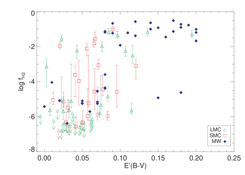
Figure 7.— Comparison of the FUSE LMC and SMC molecular fractions with the Copernicus (S77) sample of stars in the Galactic disk (MW). The SMC and LMC points have been given small random shifts in foreground-corrected color excess of up to E^′(B-V) = $\pm$0.003 to separate coincident points. Below E^′(B-V) = 0.08, the scatter in molecular fraction is large in the Clouds. For E^′(B-V) $\geq 0.10$, the SMC and LMC points lie below the average Galactic value of $f_{\rm H2}$ $\simeq 0.1$.

Figure 8.— Left panel: Molecular fraction versus total H column density for the 44 LMC and 26 SMC sight lines and the S77 sample. Right panel: Cumulative average molecular fraction for the LMC, SMC, and S77 samples, as a function of the maximum value of the total gas content, N(H) = N(H I) + 2N(H₂), considered in the average. The LMC and SMC are more gas-rich than the Galaxy, but they have a lower molecular fraction.

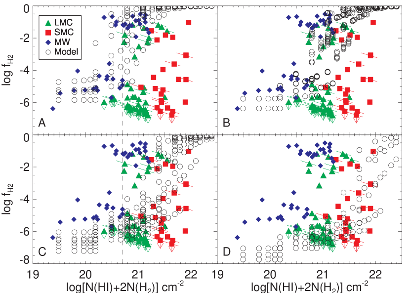
Figure 9.— The S77, LMC, and SMC samples plotted against the total H content and compared to our numerical models. The panels are labeled with the letter of the model grids they display (see Table 7). Panel A: These models have Galactic values of $R$, $I$, and the full range of kinetic temperature, gas density, and cloud size. Panel B: As before, but with $R=3\times 10^{-18}$ cm³ s^-1, 0.1 times Galactic. Panel C: Same as before, with Galactic $R$ and $I=10-100\times$ the Galactic value. Panel D: As before, but with $R=3\times 10^{-18}$ cm³ s^-1 and $I=10-100\times$ the Galactic value. The agreement with the LMC and SMC data indicates enhanced radiation and reduced H₂ formation rate in the Clouds. See § 3.2 for more discussion. The error bars are attached randomly to half the points to account for the systematic uncertainty in N(H I).

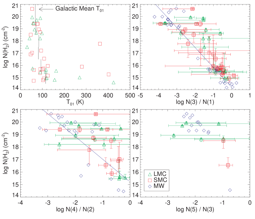
Figure 10.— Upper left: Rotational temperature $T_{01}$ plotted against total H₂ column density N(H₂). We find $\langle T_{01}\rangle=82\pm 21$ K for sight lines with N(H₂) $\geq 10^{16.5}$ cm^-2 (excluding the outlier AV 47 in the SMC) and $\langle T_{01}\rangle=115$ K for all sight lines. The rotational temperatures for LMC and SMC sight lines lie near the Galactic average of $77\pm 17$ K from S77, indicating that the physical conditions in LMC and SMC gas may be similar to those in the Galaxy if $T_{01}$ traces the kinetic temperature for high column density clouds. Upper right: The column density ratio N(3)/N(1) for the LMC and SMC samples, compared with the Galactic sample. There is no evidence for enhanced N(3)/N(1) in the Clouds, perhaps indicating that this ratio is determined by collisions at densities similar to those in Galactic gas. The blue lines are fits to the Galactic points. Lower left: The column density ratio N(4)/N(2) for the LMC and SMC samples, compared with the Galactic sample. Lower right: The column density ratio N(5)/N(3) for the LMC and SMC samples, compared with the Galactic sample.

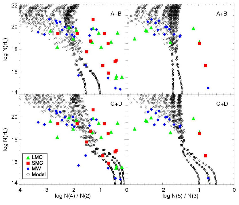
Figure 11.— The column density ratios N(4)/N(2) and N(5)/N(3) for the LMC, SMC, and Galactic samples, compared with the model grid (in open circles). The model grids plotted have the range of density, size, temperature, and incident radiation field discussed in § 3.2. The LMC and SMC samples show considerable rotational excitation above the Galactic observations and the models. In general, increasing incident radiation and decreasing formation rate coefficient $R$ move model points to the lower right on this diagram.

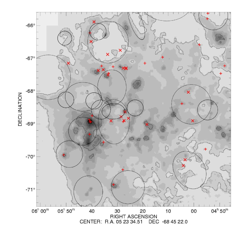
Figure 12.— IRAS 100 $\mu$m map of the LMC (Wheelock et al. 1991), showing the survey targets. A $+$ sign marks a detection, and $\times$ symbol designates a non-detection. The contours are values of 10, 100, and 1000 MJy sr^-1. In the LMC, there are 23 detections of H₂ in 44 sight lines. Aside from the strong detections of H₂ around 30 Doradus (near 5^h 40^m, -69^∘), there is no correlation between IRAS flux and H₂ column density at a given position. The ovals mark the positions of the 22 H I supershells identified by Kim et al. (1999). The patchy nature of the LMC interstellar medium and superbubble blowouts may explain the low H₂ detection rate in the LMC.

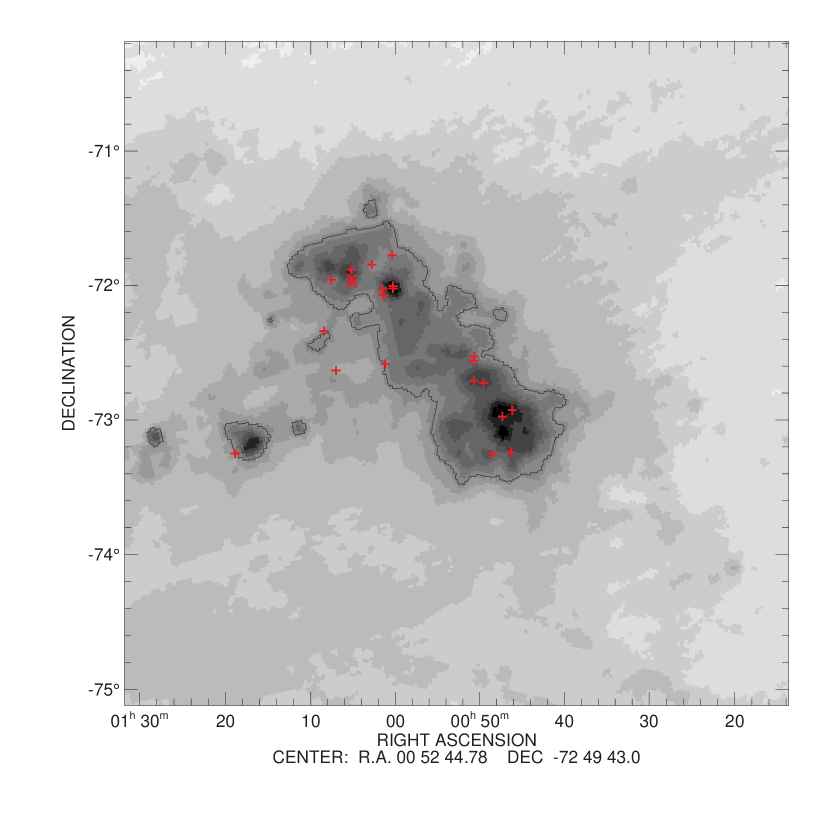
Figure 13.— IRAS 100 $\mu$m map of the SMC (Wheelock et al. 1991), showing the locations of the survey targets. A $+$ sign marks a detection of H₂, and $\times$ symbol designates a non-detection. The contours are values of 10, 100, and 1000 MJy sr^-1. In the SMC, there are 24 detections in 26 sight lines.

Figure 14.— No correlation is found between IRAS 100 $\mu$m surface brightness, $\sigma_{\rm FIR}$, of the LMC CO clouds (Cohen et al. 1988) and N(H₂) measured with FUSE. The method of Israel (1997) for deriving H₂ column densities from far-infrared flux is compared to the pencil-beam FUSE survey as discussed in the text. No correlation is found between IRAS 100 $\mu$m flux and N(H₂) measured with FUSE. The total H₂ mass for the LMC extrapolated from the FUSE sample lies $10\times$ below the mass inferred by Israel (1997). This indicates a significantly lower molecular content in the LMC or a substantial cold, dense component not sampled by the FUSE sample.

References

- (1) Abgrall, H., Roueff, E., Launay, F., Roncin, J. Y., Subtil, J. L. 1993a, A&AS 101, 273
- (2) Abgrall, H., Roueff, E., Launay, F., Roncin, J. Y., Subtil, J. L. 1993b, A&AS 101, 323
- (3) Black, J. H., Chaffee, F. H., Jr., & Foltz, C. B. 1987, ApJ 317, 442
- (4) Bevington, P. R., & Robinson, D. K. 1992, Data Reduction and Error Analysis in the Physical Sciences (New York: McGraw-Hill)
- (5) Breysacher, J., Azzopardi, M., & Testor, G. 1999, A&AS, 137, 117
- (6) Carruthers, G. 1970, ApJ, 161, L81
- (7) Cohen, R. S., Dame, T. M., Garay, G., Montani, J., Rubio, M., Thaddeus, P. 1988, ApJ, 331, 95
- (8) Conti, P. S., Garmany, C. D., & Massey, P. 1986, AJ, 92, 48
- (9) Crampton, D., & Greasley, J. 1982, PASP, 94, 31
- (10) Crowther, P. A., Hillier, D. J., & Smith, L. J. 1995, A&A, 293, 172
- (11) Crowther, P. A., & Smith, L. J. 1997, A&A, 320, 500
- (12) Crowther, P. A., De Marco, O., & Barlow, M. J. 1998, MNRAS, 296, 367
- (13)
- (14) Danforth, C. W., Howk, J. C., Sembach, K. S., & Blair, W. P. 2001, ApJS, in preparation
- (15) Dixon, W. V., Hurwitz, M., & Bowyer, S. 1998, ApJ, 492, 569
- (16) Fitzgerald, M. P. 1970, A&A, 4, 234
- (17) Fukui, Y., et al. 1999, PASJ, 51, 745
- (18) Garmany, C. D., Conti, P. S., & Massey, P. 1987, AJ, 93, 1070
- (19) Garmany, C. D., & Walborn, N. R. 1987, PASP, 98, 240
- (20) Ge, J., & Bechtold, J. 1997, ApJ, 477, L73
- (21) Ge, J., Bechtold, J., & Kulkarni, V. 2001, 547, L1
- (22) Gunderson, K. S., Clayton, G. C., & Green, J. C. 1998, PASP, 110, 60
- (23) Fitzpatrick, E. L. 1985, ApJS, 59, 77
- (24) Fitzpatrick, E. L. 1988, ApJ, 335, 703
- (25) Friedman, S., et al. 2000, ApJ, 538, L39
- (26) Hollenbach, D. J., & McKee, C. F. 1979, ApJS, 41, 555
- (27) Hollenbach, D. J., Werner, D., & Salpeter, E. E. 1971, ApJ, 163, 165
- (28) Israel, F. P., De Grauuw, Th., Lidholm, S., Van de Stadt, H., & De Vries, C. P. 1982, ApJ, 262, 100
- (29) Israel, F. P., De Grauuw, Th., Van de Stadt, H., & De Vries, C. P. 1986, ApJ, 303, 186
- (30) Israel, F. P., et al. 1993, A&A, 276, 25
- (31) Israel, F. P. 1997, A&A, 328, 471
- (32) Jenkins, E. B., & Peimbert, M. 1997, ApJ, 477, 265
- (33) Jenkins, E. B., Wozniak, P. R., Sofia, U. J., Sonneborn, G., & Tripp, T. M. 2000, ApJ, 538, 275
- (34) Jura, M. 1974, ApJ, 191, 375
- (35) Jura, M. 1975a, ApJ, 197, 575
- (36) Jura, M. 1975b, ApJ, 197, 581
- (37) Kim, S., Dopita, M. A., Staveley-Smith, L., & Bessell, M. S. 1999, AJ, 118, 2797
- (38) Koenigsberger, G., Moffat, A. F. J., St-Louis, N., Auer, L. H., Drissen, L., & Seggewiss, W. 1994, ApJ, 436, 301
- (39) Koornneef, J. 1982, A&A, 107, 247
- (40) Lennon, D. J. 1997, A&A, 317, 871
- (41) Lequeux, J., Le Bourlot, J., Des Forets, G., Roueff, E., & Boulanger, F., & Rubio, M. 1994, A&A, 292, 371
- (42) Mallouris, C., et al. 2001, ApJ, 558, 133
- (43) Maloney, P., & Black, J. H. 1988, ApJ, 325, 389
- (44) Moffat, A. F. J., Niemela, V. S., & Marraco, H. G. 1990, ApJ, 348, 232
- (45) Moos, H. W., et al. 2000, ApJ, 538, L1
- (46) Petitjean, P., Srianand, R., & Ledoux, C. 2000, A&A, 354, L26
- (47) Rachford, B. L., et al. 2001, ApJ, 555, in press
- (48) Richter, P. 2000, A&A, 359, 1111
- (49) Rousseau, J., Martin, N., Prévot, L., Rebeirot, E., Robin, A., & Brunet, J. P. 1978, A&AS, 31, 243
- (50) Rubio, M., Lequeux, J., & Boulanger, F. 1993, A&A, 271, 9
- (51) Ryu, K. S., Dixon, W. V., Hurwitz, M., Seon, K. I., Min, K. W., Edelstein, J. 2000, ApJ, 529, 251
- (52) Sahnow, D., et al. 2000, ApJ, 538, L7
- (53) Savage, B. D., Bohlin, R. C., Drake, J. F., & Budich, W. 1977, ApJ, 216, 291 (S77)
- (54) Schlegel, D., Finkbeiner, D., & Davis, M. 1998, ApJ, 500, 525
- (55) Shull, J. M., et al. 2000, ApJ, 538, L73
- (56) Shull, J. M., & Beckwith, S. V. W. 1982, ARA&A, 20, 163
- (57) Shull, J. M., & van Steenberg, M. E. 1985, ApJ, 294, 599
- (58) Smith, L. J., Shara, M. M., & Moffat, A. F. J. 1996, MNRAS, 281, 163
- (59) Snow, T. P., et al. 2000, ApJ, 538, L65
- (60) Spitzer, L., Jr., Cochran, W. D., & Hirshfeld, A. 1974, ApJS, 28, 373
- (61) Stanamirovic, S., Staveley-Smith, L., Dickey, J. M., Sault, R. J., & Snowden, S. L. 1999, MNRAS, 302, 417
- (62) Staveley-Smith, L. et al. 2001, in preparation
- (63) Torres-Dodgen, A. V., & Massey, P. 1988, AJ, 96, 1076
- (64) van Dishoeck, E., & Black, J. H. 1986, ApJS, 62, 109
- (65) Walborn, N. R. 1977, ApJ, 215, 53
- (66) Walborn, N. R. 1982, ApJ, 254, L15
- (67) Walborn, N. R. 1983, ApJ, 265, 716
- (68) Walborn, N. R., & Blades, J. C. 1986, ApJ, 304, L17
- (69) Walborn, N. R., & Blades, J. C. 1997, ApJS, 112, 457
- (70) Walborn, N. R., Lennon, D. J., Haser, S. M., Kudritzki, R.-P., & Voels, S. A. 1995, PASP, 107, 104
- (71) Walborn, N. R., Lennon, D. J., Heap, S. R., Lindler, D. J., Smith, L. J., Evans, C. J., & Parker, J. W. 2000, PASP, 112, 1243
- (72) Walborn, N. R., Fullerton, A. W., Crowther, P. A., et al. 2001a, in preparation
- (73) Walborn, N. R., Howarth, I. D., Lennon, D. J., et al. 2001b, AJ, submitted
- (74) Welty, D. E., Lauroesch, J. T., Blades, J. C., Hobbs, L. M., & York, D. G. 1997, ApJ, 489, 672
- (75) Welty, D. E., Frisch, P. C., Sonneborn, G., & York, D. G. 1999, ApJ, 512, 636
- (76) Wheelock, S. L., et al., 1991, IRAS Sky Survey Atlas Explanatory Supplement