The Epoch of Galaxy Formation

Abstract

I present a biased review of when the epoch of formation of galaxies (both disks and ellipticals) maybe took place. I base my arguments in simple (mostly) analytic models that have been recently developed to reproduce most of the observed photometric, chemical and dynamical properties of galaxies both at low and high redshift.

Dept of Physics & Astronomy, Rutgers University, 136 Frelinghuysen Road, Piscataway NJ 08854. raulj@physics.rutgers.edu

1. Introduction

A much sought after “holy grail” of cosmology is the epoch of galaxy formation. Not only it will give us information about when the intergalactic and intercluster medium was enriched (see this volume) but also allows us to test (extremely) opposed scenarios of galaxy formation and the nature of the initial conditions (e.g. Verde et al. 2001).

The most direct method to compute the different predictions of galaxy formation models consists in simulating in a computer the processes of galaxy formation and evolution from different sets of initial conditions. Unfortunately, the limitations in both computer power and our knowledge of physics to simulate the dynamics of the gas and somehow the dark matter itself, makes this approach inconclusive as to what is the epoch of galaxy formation (see e.g. Ellis 2001). On the other hand, great insight can be gained in understanding this epoch by using simple analytic models of galaxy formation, that include robust predictions from theory, and combining them with observations to constrain the free parameters in the model. In the next two sections I describe some progress using this hybrid approach in understanding the epoch of galaxy formation for both disk and elliptical galaxies.

2. Disk Galaxies

Many authors have investigated galactosynthesis models for disk galaxies, both locally and at high redshift, (e.g., Einseistein & Loeb 1996; Dalcanton, Spergel & Summers 1997; Mo, Mao & White 1998; Jimenez et al. 1998; Avila–Reese et al. 1999; Somerville & Primack 1999; van den Bosch 2000; Firmani & Avila-Reese 2000; Mo & Mao 2000; Navarro & Steinmetz 2000; Bullock et al. 2001; Boissier et al. 2001) in which the properties of disk galaxies are determined primarily by the mass, size, and angular momenta of the halos in which they form, and which may contain the effects of supernova feedback, adiabatic disk contraction, cooling, merging, and a variety of star-formation (SF) recipes. Additionally Buchalter, Jimenez & Kamionkowski (2001), investigated a variety of galactosynthesis models with realistic stellar populations and made multi-wavelength predictions for the Tully-Fisher (TF) relation. With reasonable values for various cosmological parameters, spin ($\lambda$) distributions, formation-redshift ($z_{f}$) distributions, and no supernova feedback, they produced an excellent fit to the local TF relation at all investigated wavelengths ($B$, $R$, $I$, and $K$), as well as to $B$-band TF data at $z=1$, and to the surface-brightness–magnitude ($\mu$-$M$) relation locally and at $z=0.4$. These successes suggest that their simplified mostly analytic approach captures the essential phenomenology, even if it leaves out some of the details of more sophisticated models. Using this model with a relatively minimal set of ingredients it is possible to derive the most likely redshift of formation of disk galaxies.

Figure 1.: Predicted $B$-, $R$-, $I$-, and $K$-band TF relations at $z=0$ for the A model, high-$\Omega_{b}$ model, and low-$z_{f}$ model. The scattered dots show the results for fixed masses of $10^{10}$, $10^{11}$, $10^{12}$, and $10^{13}$ ${\cal M}_{\odot}$. The solid lines are the best-fitting TF relations, with zero points and slopes given by $a$ and $b$, respectively, while the dashed lines show the 1-$\sigma$ scatter, denoted in each plot by $\sigma$.

2.1. Mostly analytic modelling of disk galaxies

Here, I briefly review the main ingredients of the galactosynthesis model developed in Buchalter, Jimenez & Kamionkowski (2001), hereafter BJK, based in turn upon that of Heavens & Jimenez (1999). The authors used the spherical-collapse model for halos (Mo, Mao & White 1998), the distribution of halo-formation times from the merger-tree formalism (Lacey & Cole 1994), and a joint distribution in $\lambda$ and $\nu$, the peak height (Heavens & Peacock 1988). Halos were treated as isothermal spheres with a fixed baryon fraction and specific angular momentum, and their embedded gaseous disks, assumed to form at virialization, have an exponential density profile. They implicitly assumed that the halos of spiral galaxies form smoothly, rather than from major mergers. An empirical Schmidt law relates the star-formation rate (SFR) to the disk surface density (Kennicutt 1998). A Salpeter initial mass function, a prescription for chemical evolution, and a synthetic stellar-population code (Jimenez et al. 1998) provide the photometric properties of disks at any $z$.

The model is defined by cosmological parameters and by the time when the most massive progenitor contains a fraction $f$ of the present-day mass, when a halo is defined to form. They found that excellent agreement with current data was obtained by their ’Model A’, a COBE-normalized $\Lambda$CDM cosmogony with $\Omega_{0}=0.3$, $h=0.65$, $\Omega_{b}h^{2}=0.019$, an untilted power spectrum with a shape parameter given by $\Gamma=\Omega_{0}h$, and with $f=0.5$. The TF relation in this model relied on both halo properties and upon the SF history of the disk. The local TF scatter arose primarily from the $z_{f}$ distribution, and secondarily from chemical evolution and the $\nu$-$\lambda$ anticorrelation. In this model, disk formation occurs primarily at $0.5\mathrel{\hbox{\hbox to0.0pt{\hbox{\lower 4.0pt\hbox{$\sim$}}\hss}\hbox{$<$}}}z\mathrel{\hbox{\hbox to0.0pt{\hbox{\lower 4.0pt\hbox{$\sim$}}\hss}\hbox{$<$}}}2$ and the TF slope steepens and the zero points get fainter from $z=0$ to $z=1$. Moreover, the amount of gas expelled from or poured into a disk galaxy in this model is relatively small and the disk and halo specific angular momenta are equal.

The problem is that this fit is not unique and a suite of other models that give good fits to the observations at low $z$ can also be found. To illustrate, they examined two alternative models, which though less observationally favored, also meet the considerable burden of yielding comparably good fits to the slope, zero-point, and scatter of the TF relation at $z=0$ in $B$, $R$, $I$, and $K$. The first is a CDM model with $\Omega_{0}=1$, $h=0.65$, constant metallicity given by the solar value, $\lambda=0.05$ for all disks, an untilted power-spectrum with amplitude $\sigma_{8}=0.5$ and empirical shape parameter value of $\Gamma=0.2$, and $f=0.5$. As shown in BJK and elsewhere, high-$\Omega_{0}$ models generally produce disk galaxies too faint to lie on the local TF relation. To compensate for this, they assumed $\Omega_{b}h^{2}=0.045$, and termed this the ’high-$\Omega_{b}$’ model.

Their second alternative is a $\Lambda$CDM cosmogony like Model A, but with metallicity held constant at the solar value, $\lambda=0.05$ for all disks, and $f=0.9$. This results in a narrow distribution of formation times peaked around $z\sim 0.2$ (for $L_{*}$-type disks), with appreciable ongoing formation today and almost no halos forming earlier than $z=1$. They thus denoted this the ’low-$z_{f}$’ model. This model will produce extremely young and bright disks. To compensate for this, they reduced the efficiency of SF in the Schmidt-law prescription by 50%. This lower SF efficiency may be plausible given the lower disk gas fractions predicted by their A model as compared with observed values.

Figure 2.: TF predictions of the A model and high-$\Omega_{b}$ model at $z=3$. The low-$z_{f}$ model predicts essentially no disks to have formed at $z=3$ at these scales.

The left, middle, and right panels of Figure 1 respectively depict the $z=0$ predictions for the A, high-$\Omega_{b}$, and low-$z_{f}$ models, in the $B$, $R$, $I$, and $K$ bands. In each panel, the solid line shows a least-squares fit to the TF-relation prediction, with a zero-point and slope given by ’$a$’ and ’$b$’, respectively, and 1-$\sigma$ errors given by the dashed lines and denoted in each plot by ’$\sigma$’. The four scattered-dot curves in each plot trace the predicted TF spread for four fixed masses ($10^{10}$, $10^{11}$, $10^{12}$, and $10^{13}M_{\odot}$), using $\sim 120$ points each. The open symbols represent extinction-corrected data from Tully et al. (1998), comprised of spiral galaxies in the loose clusters of Ursa Major and Pisces. In each plot, the data are fit to the corresponding model, and the value of $p$ gives the probability of obtaining a value of $\chi^{2}$ as large as that measured, given that the model is correct. Since the data have excluded spirals that show evidence of merger activity or disruption, they exclude from their predictions those galaxies with $B-R<0.3$.

Each of the three models yields a reasonable fit to the slope and normalization of the TF relation in all wavebands. Moreover, the predicted scatter in the $B$, $R$, $I$, and $K$ bands roughly agrees with the observed values of 0.50, 0.41, 0.40, and 0.41, respectively. Yet the epoch of disk formation is rather different in these three scenarios.

A way to break this degeneracy is to study the evolution of the TF relation with redshift. The evolution of the TF relation, and in particular its scatter, which owes to different mechanisms as one looks at different wavebands and/or at different epochs, can probe the spread in halo $z_{f}$, as well as SF processes in the disk. Specifically, for local observations of evolved systems at redder wavelengths, the scatter essentially decouples from the luminosity axis since the light is tracing the total mass roughly independently of the galaxy’s age. By contrast, observations at high $z$ and/or in bluer bands are more sensitive to the disk’s age, resulting in a scatter that couples more closely to the luminosity axis of the TF relation, decoupling almost entirely from the $V_{c}$ axis in the case of very young systems at $z=3$ (see Figure 2).

3. Spheroidal Galaxies

Spheroidal galaxies are the main contributors to the enrichment of the intergalactic medium. Therefore it is important to know when they formed. Furthermore, field elliptical galaxies can be used to test (extremely) opposed models of galaxy formation. The most obvious way to discover the epoch of spheroid formation is to find the most distant objects with spheroid morphology. This can be difficult for two reasons: first, the morphology of a forming spheroid for the first couple of Gyr may not be that of a spheroid, due to strong feedback from recently formed stars and winds (e.g. Jimenez et al. 1999; Pettini et al. 2001). Second, it might be extremely difficult to find these progenitors due to their intrinsic low surface brightness; e.g. a local elliptical galaxy becomes invisible for the HST at a redshift larger than 2. Fortunately, some other indirect routes exist. The most obvious one is to date the stellar population of the spheroid galaxy from its composite stellar spectrum. This requires very good $S/N$ spectrum and good stellar population models. The dating of nearby ellipticals has been attempted recently by concentrating on features that break the age–metallicity degeneracy (e.g. Vazdekis & Arimoto 1999; Trager et al. 2000) . This dating has been done in the context of single stellar populations, i.e. it is assumed that the elliptical galaxy is formed in a single burst of infinitesimal duration at a given age for a single metallicity. Since any tiny amount of star formation ($>5$%) will dominate the optical spectrum, this method is not optimal at determining the age of the oldest stars in the elliptical galaxy. In fact, a wide range of ages for local elliptical galaxies has been reported in these studies. A more fruitful approach is to treat the star formation rate in elliptical galaxies as a free parameter and try to do a multi-parameter fit to the observed spectrum, this was attempted by Reichardt, Jimenez & Heavens (2001). In this work the authors found that most elliptical galaxies in the small Kennicutt sample (Kennicutt 1992) had recent star formation activity albeit at a very low level ($\sim 5\%$), but the bulk of the population was formed at a redshift higher than 2. Of course, the dating of the stellar population can be done more successfully by looking at the most distant objects that exhibit spheroid morphology at high–redshift, since then it is easier to date the stellar population both because it is young and also should be free of posteriori episodes of star formation. This has been done recently by Dunlop et al. (1996), Spinrad et al. (1997), Dunlop (1999) and Nolan et al. (2001) for two red spheroidal systems at high–redshift. The ages of these objects yield a redshift of formation, for this particular class of galaxies, larger than 4. A different approach consists in using a simple but physically motivated model to fit observational properties of elliptical galaxies in order to determine their formation redshift. I devote the rest of this section to describe such a model developed in Menanteau, Jimenez & Matteucci (2001).

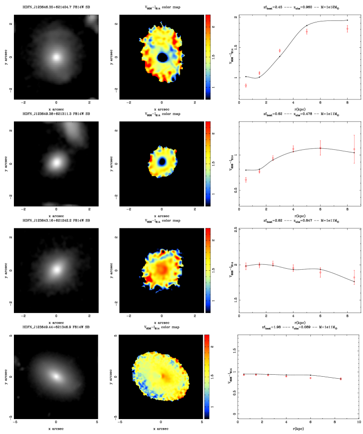
Figure 3.: An example of the ability of the model to reproduce a range of different color gradients. Figure shows from left to right: $I_{814}$–band surface brightness map, $V_{606}-I_{814}$ color pixel map and $V_{606}-I_{814}(r)$ color gradient. Open circle represent observed gradients while solid line model prediction.

3.1. Multi–zone modelling of elliptical galaxies

In a recent paper (Menanteau, Jimenez & Matteucci 2001), elliptical galaxies were modelled as a system with spherical symmetry and multiple zones. In particular it is assumed that the bulk ($>80\%$) of the gas in this model was in place at the time of formation and was able to form stars, i.e. was cool enough. The galaxy is then divided in spherical shells –100 for the present case– each of them independent, i.e. no transfer of gas is allowed among shells. In each of these shells star formation proceeds according to a Schmidt law: SFR$=\nu\rho_{\rm gas}(t)$, where $\rho_{\rm gas}(t)$ is the volume gas density in the shell and $\nu=8.6(M_{\rm gas}/10^{12}M_{\odot})^{-0.115}$Gyr^-1. The initial mass function is assumed to be a power law ($\phi(m)\propto m^{-0.95}$). Star formation proceeds in each shell until the gas is heated up by SN to a temperature $T$ that corresponds to the escape velocity of each shell (see Martinelli, Matteucci & Colafrancesco (2000) for a detailed description of the model). The gas in the elliptical galaxy is assumed to be within a dark matter halo of mass 7 times larger than the gas mass ($\Omega_{m}=0.35$ and $\Omega_{b}=0.05$). The dark matter follows the density profile described in Martinelli, Matteucci & Colafrancesco (2000). The chemical enrichment of the gas and stars is followed in detail using up–to–date nucleosynthesis prescriptions and taking into account the stars lifetimes. For each shell it is assumed that mixing of the gas is very efficient in the whole shell and shorter than the lifetime of the most massive stars.

For different masses the model predicts a different time dependence of the SFR. In more massive systems the potential well will be deeper and therefore it will take longer for the gas to reach temperatures larger than the escape velocity in the potential, thus star formation will last longer than in less massive systems. Also, for a fixed mass, since the potential is deeper in the core of the galaxy, the model predicts that star formation will last longer in the core than in the outer regions (see Martinelli, Matteucci & Colafrancesco (2000)). In fact, the predicted SFR for this model is very similar to that from detailed 1-D hydrodynamical models (e.g. Jimenez et al. (1999)). Knowing the star formation rate and chemical composition for each radii, it is then possible to compute the spectral properties of the galaxy by using a synthetic stellar population code (Jimenez et al. 1998).

3.2. Results

The aim of Menanteau, Jimenez & Matteucci (2001) analysis was to directly compare the observed $V_{606}-I_{814}(r)$ color gradients with the predictions of the above model. Once the stellar mass of the galaxy is determined from matching the $I-$band observations, the only free parameter now in their model is the redshift of formation. To accomplish this they used a maximum likelihood method ($\chi^{2}$) to compute the most-likely redshift of formation ($z_{\rm F}^{\rm best}$) for the best-fitting model. In order to avoid spurious results from small fluctuations in the gradients due to noise, the model and data gradients were re-binned to a common grid of $5-6$ shells up to a maximum physical radius of $10$ kpc. In order to transform the observed color gradients to physical (kpc) length, they assumed a flat cosmology with $\Omega_{m}=0.35$ and $H_{0}=65$ km s^-1 Mpc^-1.

They applied this methodology to the whole sample of 77 E/S0 galaxies from the HDFs. Figure 3 shows a selection of four representative galaxies in the sample. It can be seen how the model can successfully account for the observed range of $V_{606}-I_{814}(r)$ color gradients. It is worth noting the ability of the model to reproduce the blue cores (inverse steep gradients) present in the sample (Figure 3 upper two panels), both the color difference and the physical scale at which this occurs. In addition very flat and smooth color profiles can be successfully reproduced (Figure 3 lower two panels) as expected from a stellar population formed in single burst at high redshift.

Since the redshift of formation was the only free parameter in their analysis, using the HDFs it was possible to determine this parameter within the context of the above model. Figure 4 shows the distribution of the formation redshift for the whole sample. The top axis shows the look–back–time. About 25% of field E/S0 in their sample have formed at $z>4$, with $\sim 30\%$ of the sample having formed at $z<1$. The medium redshift of formation is $z\sim 2$ and therefore the medium age of the field ellipticals in the HDFs is $\sim 11$ Gyr. Therefore, as a whole, field ellipticals are only 1–2 Gyr younger than cluster ellipticals, in agreement with the findings by Bernardi et al. (1998) who compared the Mg${}_{2}-\sigma_{0}$ relation for field and cluster ellipticals. The main feature of fig. 4 is the continuous formation of field E/S0 with redshift, they did not find evidence for a single epoch of spheroid formation. This result should not be over interpreted though, due to the fact that the HDFs cover a very small area of the sky and a large number of highly clustered red objects have been found in larger area surveys (Cimatti et al. 1999; McCarthy et al. 2000). It will be interesting to see what color gradients these galaxies have and check weather or not inverse color gradients are a common feature among elliptical galaxies at high redshift.

Figure 4.: Histogram for the most likely redshift of formation, $z_{F}$ values for the whole sample of E/S0.

4. Conclusions

I have argued that using simple (mostly) analytic models of galaxy formation it is possible to understand the epoch of galaxy formation. The Tully-Fischer relation gives us strong constraints as when the big disks we see today can be assembled. Using this argument the most likely redshift of formation for present disks is at $0.5\mathrel{\hbox{\hbox to0.0pt{\hbox{\lower 4.0pt\hbox{$\sim$}}\hss}\hbox{$<$}}}z\mathrel{\hbox{\hbox to0.0pt{\hbox{\lower 4.0pt\hbox{$\sim$}}\hss}\hbox{$<$}}}2$. On the other hand, it has become apparent in recent years that elliptical galaxies are not the simple systems once were thought to be, i.e. single burst systems formed at high redshift. In fact, it has been shown that some fraction of elliptical galaxies show evidence of current star formation. Using a multi-zone model to describe the formation of elliptical galaxies and that successfully fits the color (and metallicity) gradients observed for spheroids in the HDF, I have argued that there is not a single epoch for the formation of spheroids and that it is better described as a continuous process, although about 50% of the spheroids seem to have formed at a very high redshift ($z>4$). Indeed, new telescopes (like SIRTF and NGST) will shed new light on the epoch of galaxy formation issue.

Acknowledgments.

It is a pleasure to acknowledge my collaborators in this work: Ari Buchalter, Marc Kamionkowski, Francesca Matteucci and Felipe Menanteau.

References

Avila-Reese V., Firmani C., Klypin A., Kravtsov A., 1999.MNRAS, 310, 527.

Bernardi M. et al., 1998. ApJ, 508, L143.

Boissier S., Boselli A., Prantzos N., Gavazzi G., 2001, MNRAS, 321, 733.

Buchalter A., Jimenez R., Kamionkowski M., 2001. MNRAS, 322, 43.

Bullock J. S. et al., 2001.MNRAS, 321, 559.

Cimatti A. et al., 1999. A&A, 352, L45.

Dalcanton J. J., Spergel D. N., Summers F. J., 1997.ApJ, 482, 659.

Dunlop J.S., Peacock J.A., Spinrad H., Dey A., Jimenez R., Stern D., Windhorst R., 1996. Nature, 381, 581.

Eisenstein D. J., Loeb A., 1996.ApJ, 459, 432.

Ellis R.S., 2001, astro-ph/0102056.

Firmani C., Avila-Reese V., 2000.MNRAS, 315, 457.

Heavens A., Peacock J., 1988. MNRAS, 232, 339.

Heavens A., Jimenez R., 1999. MNRAS, 305, 770.

Jimenez R., Friaca A., Dunlop J.S., Terlevich R.J., Peacock J.A., Nolan L.A., 1999. MNRAS, 305, 770.

Jimenez R., Padoan P., Matteucci F., Heavens A., 1998. MNRAS, 299, 123.

Kennicutt R. C., 1992. ApJSS, 79, 255.

Kennicutt R. C., 1998. ApJ, 498, 541.

Lacey C., Cole S., 1994. MNRAS, 271, 676.

McCarthy P. et al., 2000. astro-ph/0011499.

Martinelli A., Matteucci F., Colafrancesco S., 2000. A&A, 354, 387

Menanteau F., Jimenez R., Matteucci F., 2001. Submitted to ApJ.

Mo H. J. & Mao S., 2000.MNRAS, 318, 163.

Mo H.J., Mao S., White S.D.M., 1998. MNRAS, 295, 319.

Navarro J. F., Steinmetz M., 2000.astro-ph, 0001003.

Nolan L.A., Dunlop J., Jimenez R., Heavens J.S., 2001, astro-ph/0103450.

Pettini M. et al., 2001. astro-ph/0102456.

Reichardt C., Jimenez R., Heavens A., 2001. MNRAS in press, astro-ph/0101074.

Somerville R. S., Primack J. R., 1999.MNRAS, 310, 1087.

Spinrad H., Dey A., Stern D., Dunlop J., Peacock J.A., Jimenez R., Windhorst R., 1997. ApJ, 484, 581.

Trager S.C., Faber S.M., Worthey G., Gonzalez J.J., 2000. AJ, 119, 1645.

Tully R. B., et al., 1998. AJ, 115, 2264.

van den Bosch F. C., 2000.ApJ, 530, 177.

Vazdekis A., Arimoto N., 1999. ApJ, 525, 144.

Verde L., Jimenez R., Kamionkowski M., Materrese S., 2001. MNRAS in press. astro-ph/0011180.