Large–Scale Structure Studies with Clusters of Galaxies

Abstract

I present here a review of Large-Scale Structure (LSS) studies using clusters of galaxies. First, I re-evaluate the ‘pros’ and ‘cons’ of using clusters for such studies, especially in this era of large galaxy redshift surveys. Secondly, I provide an historical review of the Cluster Correlation Function and show that the latest measurements of $\xi_{cc}$ from Abell and X–ray catalogs are in excellent agreement. Thirdly, I review the latest measurements of the power spectrum of clusters which provide strong constraints on the cosmological parameters (e.g. $\Omega_{m}$) and models of structure formation. Moreover, I highlight the recent discovery of “Baryon Wiggles” in the local cluster p(k) which is in perfect agreement with the recent CMB data. Lastly, I examine recent advances in the measurement of the X–ray Cluster Luminosity Function and emphasize the importance of accurately determining the selection function of future cluster surveys.

Dept. of Physics, Carnegie Mellon University, 5000 Forbes Ave., Pittsburgh, PA-15232

1. Introduction

I present here an incomplete and personal review of Large-Scale Structure (LSS) studies using clusters of galaxies. For a more complete overview of clusters as cosmological probes, the reader is referred to several excellent recent reviews by Biviano (2000), Schindler (2001a), Borgani & Guzzo (2001), Guzzo (2001) and Haiman, Mohr & Holder (2001).

1.1. Pros and Cons of Using Clusters for LSS Studies

As cosmologists, we want to study and understand the distribution of matter in the Universe as a function of space and time i.e. mass(x,y,z,t). This will allow us to constrain cosmological parameters, models of structure formation as well as understanding the physical processes that control the distribution of baryons. Ultimately, we want to directly compare our observations of the Universe to cosmological simulations e.g. the VIRGO-GIF project (Kauffmann et al. 1999). This is hard to do since we need to know how the light we observe, traces the underlying matter we simulate.

Historically, clusters of galaxies have been used for this task because: a) They survey large volumes of space thus producing a fair sample of the Universe; b) Clusters can be seen over a large range in redshift, thus probing cosmological evolution; c) They maintain the imprint of the initial conditions so simple analytical relationships can be used to explain their properties (e.g. Jenkins et al. 2001); d) Clusters are the largest gravitationally bound objects in the Universe, so we can weigh the Cosmos using them; e) Clusters are full of hot baryons, so we can study how mass follows light on cluster scales.

However, clusters do have their problems. First, they live in the tail of the underlying mass distribution and thus may be highly biased tracers of this distribution. This has been a major concern for a long time (Kaiser 1986), but recent observational and theoretical work (see Miller et al. 2001a, Narayanan et al. 2000) shows that a simple linear biasing model ($b=1.5$), between normal galaxies and clusters, does work well over an important range of scales ($0.03\leq k\leq 0.15h^{-1}\,{\rm Mpc^{-1}}$. As an aside, I note that because of this fact, clusters may be an excellent probe of the gaussianity of the Universe since our models and simulations of the Universe assume gaussianity at the beginning (e.g. Chiu, Ostriker, & Strauss 1998; Robinson, Gawiser & Silk 1999; Matarrese, Verde & Jimenez 2000; Kerscher et al. 2001). Kerscher et al. (2001) has already found statistical evidence for non-gaussianity based on the REFLEX sample of X–ray clusters, although Verde et al. (2001) highlight that the CMB and high redshift galaxies maybe a better way to studying this issue.

Another concern with clusters is the assumption of hydrostatic equilbrium (for the gas) and the virial theorem (for the galaxies). For example, in the recent hydrodynamical/N-body simulations of Ricker & Sarazin (2001), an off-axis merger of two systems (mass ratio of 3:1) can produce large-scale turbulent motions with eddys up to several 100 kpcs. Even after nearly a Hubble time, these motions persist as subsonic turbulence in the cluster cores, providing 5-10% of the support against gravity. Roettiger, Burns & Loken (1996) and Ritchie & Thomas (2001) also found that major merger events can knock the cluster out of hydrostatic equilibrium for several Gyrs (see Schindler et al. 2001b for a recent review of cluster simulations).

To assess the importance of such mergers on the whole cluster population, I show in Fig. 1 the expected fraction of clusters ($M\geq 10^{14}\,M_{\odot}$ or $L_{\rm x}(0.5-2.0)>10^{43}\,{\rm erg/s}$) that have experienced a merger in the last 2.5Gyrs. This figure shows that as we push to higher redshifts the vast majority of clusters should show significant evidence for a recent merger that may severely effect their physical state (see Mathiesen & Evrard 2001). Fig. 1 is in agreement with the recent Chandra observations reported in Henry (2001) where 75% of $z>0.75$ clusters showed significant substructure. Therefore, if we wish to continue to use clusters as cosmological tracers, we must understand such effects in greater detail.

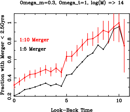
Figure 1.: The fraction of $M\geq 10^{14}\,M_{\odot}$ clusters that have experienced a major merger in the last 2.5Gyrs versus look-back time. The red points are for a 10:1 merger, while the black points are for a 5:1. These data were kindly provided by Joanne Cohn based on simulations similar to the work presented in Cohn, Bagla & White (2000). The simulations use $\Omega_{m}=0.3$, $\Omega_{\Lambda}=0.7$ and $\sigma_{8}=0.9$. The error bars are $\sqrt{N}$ of clusters detected in the simulations. For clarity, they are not shown for the 5:1 simulations.

In light of these concerns, I challenged the audience at the conference to discuss the following question over the coffee break: “In this era of galaxy redshift, lensing and photometric surveys, is there still a need for cluster surveys of the Universe?”. For example, in Fig. 2, I show initial results from the Sloan Digital Sky Survey (SDSS) Luminous Red Galaxy (LRG) survey which is designed to create a pseudo–volume limited sample of 100,000 giant ellipticals out to $z\sim 0.4$ (although the sample does reach out to $z\sim 0.6$). This survey will sample the LSS on Gigaparsec scales – comparable with the largest cluster surveys – well beyond the turn–over in the matter power spectrum (see Section 3). The LRGs are still biased tracers but there is compelling evidence that we can fully understand their selection function (see Eisenstein et al. 2001 for details).

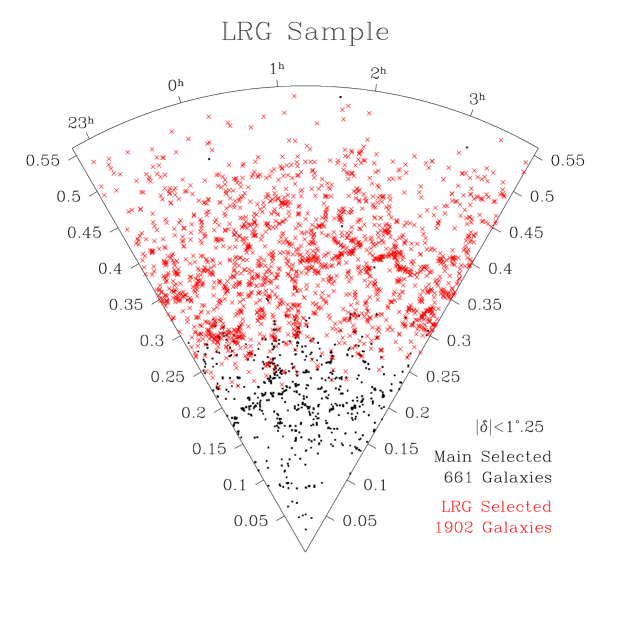
Figure 2.: Wedge plot of a small fraction of SDSS spectroscopic data collected to date. This illustrates the power of using the SDSS–LRG sample for studying the LSS. Figure kindly provided by Daniel Eisenstein.

Returning to my question, I will emphasize that clusters are still the best way to: a) Constrain $\sigma_{8}$ (see Viana & Liddle 1999); b) Determine $\Omega_{m}$ (see Sections 3 & 4), and; c) Study galaxy evolution in dense regions.

2. Cluster Correlation Function

The Cluster Correlation Function ($\xi_{cc}=(\frac{r}{r_{o}})^{-\gamma}$ where $r_{o}$ is the correlation length defined as $\xi_{cc}(r_{o})=1$) has had a long and controversial history. In the 1980’s, it was one of the main constraints on CDM models of structure formation (see White et al. 1987). The main controversy surrounding measurements of $\xi_{cc}$ has been the effects of optical projection effects on the Abell catalog i.e. the contamination of the 2D richness of clusters because of the field or a nearby clusters (Sutherland et al. 1988) and/or the super-position of two groups along the line–of–sight to create a “Phantom Cluster”. The hypothesis has been that these projection effects have artificially boosted the amplitude of Abell measurements of $\xi_{cc}$ thus making it inconsistent with CDM models (Sutherland et al. 1988; Dekel et al. 1989; Efstathiou et al. 1992). There are many advocates of this hypothesis (e.g. Dalton et al. 1992; Nichol et al. 1992 & 1994; Romer et al. 1994), but there are also many defenders of the Abell catalog (Postman et al. 1992; Miller et al. 1999). Over the last decade, such concerns have driven the creation of new optical and X–ray cluster surveys e.g. the EDCC (Lumdsen et al. 1992), APM (Dalton et al. 1992), DPOSS (Gal et al. 2000) and REFLEX surveys (Collins et al. 2000).

In Fig. 3, I show an historical overview of $\xi_{cc}$ measurements over the last 20 years. There are two interesting points to make about this figure: First, the correlation length of Abell $\xi_{cc}$’s have decreased with time. Secondly, X–ray measurements of $r_{o}$ have increased with time. These two trends can be understood via the relative space density of clusters in these different surveys. In the case of the Abell survey, the volume surveyed by the different samples of Abell clusters has not increased much since the first measurements, but the number of systems used in the measurement of $\xi_{cc}$ has steadily increased from $\sim 100$ to over $600$. Thus the space density of Abell clusters used in determining $\xi_{cc}$ has decreased over time. The opposite is true for the X–ray samples; the number of clusters used has increased, but so has the volume sampled, thus the space density has slightly decreased over time (see Croft et al 1997).

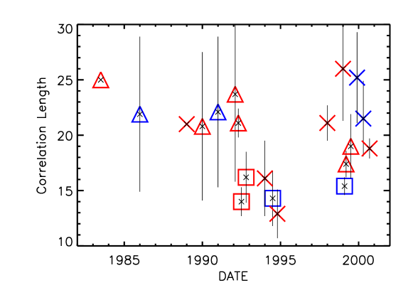
Figure 3.: The Correlation Length ($r_{o}$ in Mpc) of $\xi_{cc}$, measured by various authors, as a function of time. Triangles are Abell, squares are optical non-Abell samples and crosses are X–ray samples. Red points have a slope of the correlation function between $1.7\leq\gamma\leq 2.0$, while blue points are outside this range. Please note that I have not scaled these measurements by the space density of the cluster sample used in the measurement. I took the $r_{o}$ value and error quoted in the abstract of the papers and, in the case of multiple fits to the data, I took the $r_{o}$ from the largest sample. Data from Ling et al. 1986; West & van der Bergh (1991); Peacock & West 1992; Miller et al. 1999; Lahav et al. 1989; Romer et al. 1994; Borgani et al. 1999a; Abadi et al. 1998; Lee et al. 1999; Moscardini et al. 2000; Collins et al. 2000; Dalton et al. 1992; Nichol et al. 1992 & 1994; Postman et al. 1992; Huchra et al. 1990; Bahcall & Soneria 1983.

If we focus on recent measurements with similar slopes ($1.7\leq\gamma\leq 2.0$), then the agreement between present measurements of $\xi_{cc}$ is very good. This is illustrated in Fig. 4 where I show the $\xi_{cc}$ from nearly 1000 clusters (both Abell and X–ray). The great debate over the value of the correlation length of $\xi_{cc}$ is probably over especially given that the pi-sigma diagrams shown in Fig. 5 highlights that the clustering in both the Abell and X–ray surveys is now nearly isotropic. This removes one of the main arguments for projection effects in the Abell catalog and is probably due to the larger samples now available averaging over the effect of LSS and/or the effect of a single supercluster. We look forward to new $\xi_{cc}$ measurements from large, homogeneous samples of clusters taken from the SDSS, REFLEX and 2dF surveys.

Figure 4.: The correlation function for the Abell/ACO sample of Miller et al. (1999) and from the REFLEX sample of Collins et al. (2000). No correction has been made for the space densities of the surveys. Data kindly provided by Chris Collins and Chris Miller.

Figure 5.: The $\pi$–$\sigma$ diagrams for the two surveys presented in Fig 4. This shows the radial ($\sigma$) and transverse ($\pi$) components of the correlation function. The left–hand plot is for the REFLEX sample, while the right–hand side is from the Abell/ACO sample of Miller et al. (1999). These figures were kindly provided by Chris Collins and Chris Miller.

3. Cluster Power Spectrum

In the last ten years, many authors have switched from measuring correlation functions to measurements of the cluster power spectrum since it allows for a more direct comparison with the theoretical models. For example, increasing $\Omega_{m}h^{2}$ pushes the epoch of matter-radiation equality back in time and moves the peak in the p(k) to low k values (Tegmark 1999 ). Therefore, the detection of the turn–over in the local power spectrum (p(k)) of matter provides a powerful constrain on both the matter density of the Universe and models of structure formation (e.g. CDM).

As yet, there has been no definitive detection of a turn–over (or peak) in the local matter p(k), but we are getting close (Szalay et al. 2001; Miller et al. 2001a; Percival et al. 2001; Huterer et al. 2001) as new surveys of the local Universe are approaching volumes than demand a turn–over to satisfy the COBE measurements at very low k. This lack of a detection naturally drives estimates of $\Omega_{m}$ from these p(k)’s towards low values e.g. Miller et al. (2001a) recently estimated $\Omega_{m}\,h^{2}=0.12^{+0.03}_{-0.02}$ using a large sample of clusters to probe Gigaparsec scales. Similarly, Schuecker et al. (2001) presented the p(k) from the REFLEX sample and finds it favors low–density CDM models as the peak in the p(k) is yet undetected.

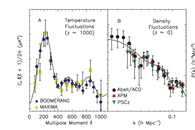
Figure 6.: On the right we show the p(k) data from clusters and galaxies as discussed by Miller et al. (2001a). The best fit model (with acoustic oscillations) is shown. On the left is the 2001 CMB balloon data. Here we plot the same model as shown on the right; this is not a fit to the CMB data. As discussed in Miller et al. (2001b), there is good agreement between the two epochs.

In addition to the hunt for the turn–over in the p(k), several authors have looked for “bumps” and “wiggles” in the local matter p(k). For example, Einasto et al. (1997) reported a “bump” in the cluster p(k) which could be do to excess power in the initial p(k) coming out of Inflation (a physical mechanism for such a feature however, remains unclear; see Atrio–Barandela et al. 2000). Alternatively, one may expect fluctuations in the observed p(k) because of the acoustic oscillation of baryons in the early Universe; sometimes called the “Baryon Wiggles”. Eisenstein et al. (1998) recently looked for this signature in the p(k) measurements from galaxy and cluster surveys but was unable to find a satisfactory fit between the cosmological models (with acoustic oscillations) and the data available at that time. This year, Miller et al. (2001a,b) and Percival et al. (2001) have revisited this problem and have found compelling evidence for the detection of the “Baryon Wiggles” in the local matter p(k) that is fully consistent with the detection of the same “Baryon Wiggles” in the recent CMB data (MAXIMA. DASI & BOOMERANG). This concordance is shown in detail in Fig. 6. In summary. in 2001, we have witnessed the simultaneous discovery of the “Baryon Wiggles” in the local ($z\sim 0.1$) and distant ($z\simeq 1000$) Universe providing yet another major success for the Hot Big Bang cosmological model.

4. The X–ray Cluster Luminosity Function

In addition to studying the clustering of clusters, it is important to understand the distribution of cluster properties (i.e. the luminosity, temperature and mass functions) and how these scale with each other and as a function of redshift. This will allow us to determine if clusters are a self–similar population (i.e. their properties can be directly predicted from using just the virial theorem and hydrostatic equilbrium, see Kaiser 1986) or are there extra contributions to the energy which breaks the simple scaling laws predicted by self-similarity. In recent years, there have been significant advances in understanding these scaling relationships (Horner et al. 1999; Sheldon et al. 2001; Mathiesen 2001; Neumann & Arnaud 2001) but we can expect continued advancements over the next decade because of new X–ray (XMM & Chandra) and lensing (Joffre et al. 2000) surveys of clusters as well as more detailed Hydro/N–body cluster simulations (see Ricker & Sarazin 2001). One example is the XMM-Newton $\Omega_{m}$ Project (Bartlett et al. 2001) which is designed to obtain accurate temperature measurements ($\simeq 10\%$ error) for all of the high redshift SHARC clusters (Romer et al. 2000; Burke et al. 1997) thus obtaining an estimate of the high redshift $L_{\rm x}$–$T_{\rm x}$ relation (over a decade in $L_{\rm x}$) as well as constraining $\Omega_{m}$.

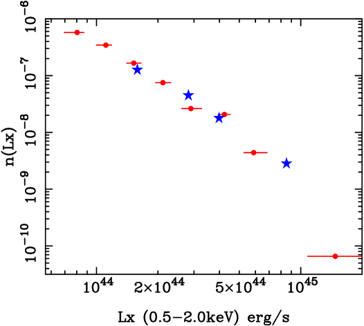
Figure 7.: The X–ray Cluster Luminosity Function for the REFLEX (red; Boehringer et al. 2001) and Bright SHARC (blue; Adami et al. 2000) cluster surveys. The REFLEX probes to $z=0.3$, while the Bright SHARC surveys the range $0.3<z\sim 0.8$. The error bars on the REFLEX sample are discussed in Boehringer et al. (2001), while a detailed analysis of the errors on the Bright SHARC are given in Adami et al. (2000) and Romer et al. (2000). The units on n(${\rm L_{x}}$) are $h^{-3}{\rm Mpc^{-3}\,(L_{x}(44))^{-1}}$. Data kindly provided by Hans Bohringer and Christophe Adami.

In the absence of a large, homogeneous sample of cluster temperatures, masses and velocity dispersions, authors have focused in recent years on the X–ray Cluster Luminosity Function (XCLF). The reader is referred to Gioia et al. (2001) and Boehringer et al. (2001) for a good recent overview of ROSAT & Einstein measurements of the XCLF as a function of redshift. The key debate with the XCLF is whether the bright–end (brighter than $L^{\star}\simeq 4\times 10^{44}\,{\rm erg/s}$) of the luminosity function has evolved since $z\sim 0.8$, thus producing a deficit of high redshift, luminous systems. As discussed by many authors, the evolution of such massive clusters is a strong constraint on $\Omega_{m}$ and thus it is vital to quantify how the luminous end of the XCLF changes with look–back time (e.g. Oukbir & Blanchard 1997; Viana & Liddle 1999; Reichart et al. 1999; Borgani et al. 1999b; Henry 2001). If $\Omega_{m}\sim 0.2$ (e.g. from p(k) of clusters above), then the amount of evolution out to $z\simeq 0.8$ should be small and thus the signal we are looking for will be weak. In this case, we must be very careful about systematic uncertainties in our distant cluster surveys. Alternatively, if $\Omega_{m}=1$, we expect approximately an order of magnitude decrease in the space density of $L_{\rm x}=10^{45}{\rm erg/s}$ systems to $z=0.8$.

In Fig. 7, I show the bright–end of the XCLF derived from the REFLEX cluster survey (Boehringer et al. 2001) and the Bright SHARC (Romer et al. 2000; Adami et al. 2000). These are two of the most well–understood surveys of X–ray clusters available to date (in terms of their selection functions etc.). The agreement between the two is remarkable but the number of luminous clusters ($>L^{\star}$) in both surveys is still relatively small because of the tiny space densities of such clusters. Furthermore, to obtain a “high precision” measurement of the XCLF, we need to carefully model the selection functions of these, and future, surveys. This was recently emphasized by Adami et al. (2000) who performed extensive simulations of the Bright SHARC selection function and found that the shape and morphology of the clusters had a dramatic effect on the efficiency of detection. When this is combined with the effect seen in Fig. 1 – i.e. that a large fraction of high redshift clusters are likely to have signs of recent interactions (see also Henry 2001) – it becomes essential to model such effects in the selection function of any distant cluster survey. Therefore, the selection functions of future surveys will need to include cosmological (e.g. $\Omega_{\Lambda}$), morphological (e.g. profile of clusters) and survey design (e.g. off-axis PSF) effects.

5. Future Cluster Surveys

As emphasized above, future cluster surveys need to improve in both quality and quantity. I highlight here four on–going efforts that will hopefully address both of these points (this is by no means a complete list). First, the MACS survey (Ebeling et al. 2001) is mining the ROSAT All–Sky Survey (RASS) for previously undiscovered high redshift ($0.3<z<0.7$) luminous clusters. The survey has been highly successful and has nearly 100 new massive clusters to date. Secondly, Gladders & Yee (2000) are embarked on a large–area ($100{\rm deg^{2}}$), two–passband, optical survey in search of high redshift clusters. Their technique makes use of the fact that cluster ellipticals are strongly clustered in color and are the reddest (rest–frame) galaxies in existence. They plan to expand their technique to $\simeq 1000{\rm deg^{2}}$.

As discussed in Romer et al. (2001), the XMM data archive will be a gold–mine for searching for distant X–ray clusters. Over the life–time of the satellite, XMM is expected to serendipitously survey $\simeq 800{\rm deg^{2}}$ which should yield thousands of cluster detections. Most importantly, the XMM Cluster Survey (XCS; Romer et al. 2001) is predicted to find zero ($\Omega_{m}=1$), twelve ($\Omega_{m}=0.3$) or fifty ($\Omega_{m}=0.3\,+\,\Omega_{\Lambda}=0.7$) massive clusters ($T_{\rm x}>6\,{\rm keV}$) at redshifts greater than one (see Romer et al. 2001). This will provide an excellent constraint on both $\Omega_{m}$ and $\Omega_{\Lambda}$ as well as providing a rich dataset of cluster temperatures and morphologies.

Finally, the Sloan Digital Sky Survey (SDSS) should produce several high quality, large–area, cluster surveys. For example, in Nichol et al. (2000), I outlined a new algorithm called “C4” which uses the 5 passband SDSS photometry and photometric redshifts, to look for clusters in a 7–dimensional space (4 colors, 2 angular, 1 radial). This removes all concerns about projection effects (see Section 2) and, when combined with the RASS data, can find clusters out to $z\simeq 0.7$.

Before I leave this section, I will emphasize again the importance of determining the selection functions of these new surveys. As the data, procedures and algorithms used in these new surveys get more complex, then we can not naively assume the volume of these surveys is just calculated from their flux limit and their area on the sky. We will need to turn to simulations of the Universe to help us e.g. using semi–analytical, N–body techniques (see Kauffmann et al. 1999) or fast analytical approximations like PTHALO (Scoccimarro & Sheth 2001). I note here that Postman (this volume) also emphasizes the need for well–understood selection functions for distant cluster surveys.

I thank the organizers of the conference for inviting me. I would like to also thank my collaborators on the SDSS, XMM–Newton $\Omega_{m}$ project, XCS and SHARC surveys. I especially thank Chris Miller, Chris Collins and Kathy Romer for their help, guidance and reading of this manuscript.

6. References

Abadi, M., et al. 1998, ApJ, 507, 526
Adami, C., et al.  2000, ApJS, 131, 391
Atrio-Barandela, F., et al. 2000, ApJL, see astro-ph/0012320
Bahcall, N. A. & Soneira, R. M. 1983, ApJ, 270, 20
Bartlett, J., et al. 2001, see astro-ph/0106098
Biviano, A., 2000, see stro-ph/0010409
Boehringer, H., et al. 2001, see astro-ph/0106243
Borgani, S., Plionis, M., & Kolokotronis, V. 1999a, MNRAS, 305, 866
Borgani, S., et al. 1999b, ApJ, 527, 561
Borgani, S. & Guzzo, L. 2001, Nature, 409, 39
Burke, D. J., et al.  1997, ApJ, 488, L83
Chiu, W. A., Ostriker, J. P., & Strauss, M. A. 1998, ApJ, 494, 479
Cohn, J. D., Bagla, J. S., & White, M. 2001, MNRAS, 325, 1053
Collins, C. A. et al. 2000, MNRAS, 319, 939
Croft, R. A. C., et al.  1997, MNRAS, 291, 305
Dalton, G. B. et al. 1992, ApJ, 390, L1
Dekel, A., Blumenthal, G. R., Primack, J. R., & Olivier, S. 1989, ApJ, 338, L5
Ebeling, H., Edge, A. C., & Henry, J. P. 2001, ApJ, 553, 668
Efstathiou, G. et al. 1992, MNRAS, 257, 125
Einasto, J., et al. 1997, Nature, 385, 139
Eisenstein, D. J., Hu, W., Silk, J., & Szalay, A. S. 1998, ApJ, 494, L1
Eisenstein, D. J., et al. see astro-ph/0108153
Gal, R. R., et al.  2000, AJ, 120, 540
Gioia, I. M., et al. 2001, ApJ, 553, L105
Gladders, M. D. & Yee, H. K. C. 2000, AJ, 120, 2148
Guzzo, L., 2001, see astro-ph/0102062
Haiman, Z., et al. 2001, see astro-ph/0103049
Henry, J. P., 2001, astro-ph/0109498
Horner, D. J., Mushotzky, R. F., & Scharf, C. A. 1999, ApJ, 520, 78
Huchra, J. P., Geller, M. J., Henry, J. P., & Postman, M. 1990, ApJ, 365, 66
Huterer, D., Knox, L., & Nichol, R. C. 2001, ApJ, 555, 547
Jenkins, A., et al. 2001, MNRAS, 321, 372
Joffre, M. et al. 2000, ApJ, 534, L131
Kaiser, N. 1986, MNRAS, 222, 323
Kauffmann, G. et al. 1999, MNRAS, 303, 188
Kerscher, M. et al. 2001, A&A, 377, 1
Lahav, O., Fabian, A. C., Edge, A. C., & Putney, A. 1989, MNRAS, 238, 881
Ling, E., Frenk, C., Barrow, J., 1986, MNRAS, 223, 21
Lumsden, S. L. et al. 1992, MNRAS, 258, 1
Matarrese, S., Verde, L., & Jimenez, R. 2000, ApJ, 541, 10
Mathiesen, B. F. 2001, MNRAS, 326, L1
Mathiesen, B. F. & Evrard, A. E. 2001, ApJ, 546, 100
Miller, C. J., Batuski, D. J., Slinglend, K. A., & Hill, J. M. 1999, ApJ, 523, 492
Miller, C. J., Nichol, R. C., & Batuski, D. J. 2001a, ApJ, 555, 68
Miller, C. J., Nichol, R. C., & Batuski, D. J. 2001b, Science, 292, 2302
Moscardini, L. et al. 2000, MNRAS, 314, 647
Narayanan, V. K., Berlind, A. A., & Weinberg, D. H. 2000, ApJ, 528, 1
Neumann, D. M. & Arnaud, M. 2001, A&A, 373, L33
Nichol, R. C., Briel, O. G., & Henry, J. P. 1994, MNRAS, 267, 771
Nichol, R. C. et al. 1992, MNRAS, 255, 21P
Nichol, R. C., et al. 2000, astro-ph/0011557
Oukbir, J. & Blanchard, A. 1997, A&A, 317, 1
Peacock, J., & West, M., MNRAS, 259, 494
Percival, W., 2001, MNRAS, see astro-ph/0105252
Postman, M., Huchra, J. P., & Geller, M. J. 1992, ApJ, 384, 404
Reichart, D. E., et al.  1999, ApJ, 518, 521
Ricker, P., Sarazin, C., 2001, ApJ, see astro-ph/0107210
Ritchie, B. W., Thomas, P. E., MNRAS, see astro-ph/0107374
Robinson, J., Gawiser, E., & Silk, J. 2000, ApJ, 532, 1
Roettiger, K., Burns, J. O., & Loken, C. 1996, ApJ, 473, 651
Romer, A. K. et al. 1994, Nature
Romer, A. K. et al. 2000, ApJS, 126, 209
Romer, A. K. et al. 2001, ApJ, 547, 594
Schindler, S., 2001a, see astro-ph/0109040
Schindler, S., 2001b, see astro-ph/0107008
Schuecker, P. et al. 2001, A&A, 368, 86
Scoccimarro, R., Sheth, R. K., 2001, see astro-ph/0106120
Sheldon, E. S. et al. 2001, ApJ, 554, 881
Sutherland, W. 1988, MNRAS, 234, 159
Szalay, A. S., 2001, ApJ, see astro-ph/0107419
Tegmark, M. 1999, ApJ, 514, L69
Verde, L. et al.  2001, MNRAS, 325, 412
Viana, P. T. P. & Liddle, A. R. 1999, MNRAS, 303, 535
West, M., & van der Bergh, S., 1991, 373, 1
White, S. D. M., Frenk, C. S., Davis, M., & Efstathiou, G. 1987, ApJ, 313, 505