Whether our universe with present day acceleration can eventually collapse is very interesting problem. We are also interesting in such problems, whether the universe is closed? Why it is so flat? How long to expend a period for a cycle of the universe? In this paper a simple “slow-fast” type of the quintessence potential is designed for the closed universe to realize the present acceleration of our universe and its eventual big collapse. A detail numerical simulation of the universe evolution demonstrates that it divides the seven stages, a very rich story. It is unexpected that the quintessential kinetic energy is dominated in the shrink stage of the universe with very rapid velocity of the energy increasing. A complete analytic analysis is given for each stage. Some very interesting new problems brought by this collapse are discussed. Therefore our model avoids naturally the future event horizon problem of the present accelerative expanding universe and maybe realize the infinite cycles of the universe, which supplies a mechanism to use naturally the anthropic principle. This paper shows that the understanding on the essence of the cosmological constant should contain a richer content.

I Introduction

The birth and termination of the universe is a riddle for mankind. An old story is that a matter-dominated closed universe will shrink finally^[1], so that the universe begins its new big bang through a bounce, and repetition forever to realize infinite kinds of universes. However, this old idea was challenged by a fact known recently, i.e., our present universe is accelerated expanding^[2]. If the reason to cause the acceleration of the universe is the real cosmological constant, then the universe will be accelerated expanding forever, never shrink in its future, thus we can not see the cycle of the universe. It is believed generally that the appearance of the wisdom life needs some kind of adjustment of some physics parameters, so that we need many worlds to realize this adjustment, that is the anthropic principle^[3]. If the universe never shrink, we have to invoke the concept of the chaotic inflation^[4]. The universe is inflating eternally in a larger region, produces many many different worlds in a fractal manner. Today this new idea is very popular in the cosmologist community. Comparing earnestly the old and new ideas, one can find out that the argument of the chaotic inflationary production of many universes owns some difficulty of mathematical description, and the old idea is more simple and clear.

We hope that our universe is accelerative in present and will shrink finally. The advantage of this idea is that the universe maybe stays in its infinite loop to realize many world scenario, that this model agrees with the present decisive astronomical observations, specially the cosmic microwave background radiation (CMBR)^[5], and that it avoid a difficulty about an event horizon for a perpetual accelerated universe^[6]. In order for the universe to shrink finally there must be some negative energy in it, for instance, a negative cosmological constant or a positive-curvature negative-energy density. In the first case we need that the cosmological constant changes from the present positive value to the future negative one, thus the cosmological constant is not a true “constant” at all. It is better for us to accept the quintessence scheme^[7], which has a good basis of the field theory. Anyhow we hope to avoid a “true cosmological constant” further, no matter what it is positive or negative, which is a big obstacle to construct a string (M-) theory^[8]. Therefore we take the vacuum of the quintessence, i.e., the minimum of its potential, to be the zero point of the energy, that is the true cosmological constant is zero absolutely for some unknown reason^[9]. The force to shrink the universe is remained only as the positive-curvature negative-energy density, i.e., the universe is closed. In spite of the universe is closed, we shall show in the section 10 that a reasonable assumption from inflation of the early universe gives a very small non-flatness of the universe, which is unobservable at present.

It is a very interesting problem how to shrink finally for a closed universe, which has acceleration at present caused by a special quintessence. It should be known that for a generic quintessence, for instance with a pure inverse power law potential or a pure exponential one, it can not arrive the above goal. That the universe is accelerative at present and will shrink in future is to require that quintessence is a “(early) slow - (late) fast (rolling)” type. However, the inverse power quintessence is a “fast-slow” type, and the exponential quintessence is a “slow-slow” or “fast-fast” ones. So that we must design a reasonable “slow-fast” quintessence. In this paper we do it in the section 2. This potential must have as simpler form and fewer parameters as possible. This special potential is called by us as “Niagara” one, since its configuration is very flat for its negative field value and falls very rapidly to the zero for its positive field value, and the quintessence rolls down from a high potential hill to a low valley without boundary.

Whether there is some new story about the evolution of the universe with our “Niagara potential”? Yes, some rich and wonderful scenario appears unexpectedly. As a typical process from the Big Bang Neucleonsythesis (BBN) to the big collapse of the universe, the evolution may be divided into seven stages, as described in the section 3. The first and second stages are the radiation and matter dominated epochs respectively, which are familiar for us. The third stage is the quintessence potential energy dominated, and the universe stays in its accelerative phase, in which the quintessence rolls slowly with its negative field value (see analysis in the sections 4-5). However, the quintessence rolls inevitably to its positive field value. When it passes through its turning point, the quintessence potential energy decreases suddenly, thus the quintessence kinetic energy will be dominated, and this is the fourth stage of the universe evolution, which is decelerated (see analysis in the section 6). Since the evolution law of the quintessence kinetic energy is faster than matter, when the cosmic scale factor expand to some value the quintessence kinetic energy will be approximately equal to the matter energy, the universe comes into its fifth phase, i.e., the “matter leading attractor” one, since its evolution law is like of matter and this new term will be explained in the section 7. Moreover, the evolution law of the matter energy is faster than the curvature energy, at some time the universe is dominated by the curvature energy, i.e., the sixth phase of the evolution (see analysis in the section 8). When the curvature negative energy cancels just all of other energies, the universe stop its expansion, and begin to shrink, i.e., the seventh phase. We note interestedly that when the universe begin to shrink, the quintessence kinetic energy, the matter one and the curvature one are all approximately equal. As the universe shrinks, the quintessence kinetic energy increase more quickly than other form energies, soon after it the quintessence kinetic energy is dominated in the collapse universe, therefore the seventh phase of the universe evolution is the “quintessence kinetic energy collapse”, it is very different from the old concept of the matter collapse (see analysis in the section 9). This will bring many interesting problems to deserve further investigation (see the section 11).

It is worth to be emphasized that it is very necessary to finish a numerical simulation in computer for a whole evolution process of the universe, otherwise we can not supply a time-scale concept for each stage and a diminishable scenario of the universe. We noted often that many seeming feasible models are actually impracticable, specially to obtain a suitable accelerative period and a reasonable age for the present universe. We give a detail result of the simulation of this seven stage evolution in this paper. We need not only the detail simulation (in the section 3), but also an analytic analysis for its essence in a manner of the quantitative estimation (in the sections 4-9).

The model parameters taken by us is only a special point of the wide parameter space in our model, however it is typical for an understanding of the essence of the evolution. To explore the various behavior of the whole parameter space is not the task of this paper. We only hope to express an idea about the present accelerated expanding universe still has a chance to shrink eventually. This opens a way to realize infinitely many universes. This kind of many universe is more simple and easy to be described in order to serve the anthropic principle. Finally we make a simple conclusion in the section 12, specially about interesting problems worth to be investigated further.

II The potential of the quintessence

We have announced that it is necessary to replace a true cosmological constant with the quintessence field $\phi$. The quintessence potential we shall take in our model has the following form

$$V(\phi)=\frac{M_{0}^{4}}{1+\exp(\lambda\phi/M_{p})}.$$ (1)

When $\phi\rightarrow-\infty$, the potential $V(\phi)$ approaches to $M_{0}^{4}$, which emulates realistically a true cosmological constant, we take $M_{0}=0.95\times 10^{-30}M_{p}$, here $M_{p}=(8\pi G)^{-1/2}$ $=2.4\times 10^{18}$GeV is the Planck energy scale. In other hand when $\phi$ is larger than zero, the potential $V(\phi)$ declines exponentially and approaches to zero quickly. The slow roll parameter of this potential is

$$\epsilon\equiv\frac{1}{2}M_{p}^{2}\frac{V^{\prime 2}}{V^{2}}=\frac{\lambda^{2}/2}{(1+e^{-\lambda\phi/M_{p}})^{2}}.$$ (2)

The parameter $\lambda$ will control the velocity of rolling. This potential is “slow-slow” type for $\lambda<\sqrt{2}$ and “slow-fast” one for $\lambda>\sqrt{2}$. In our model we take $\lambda=2$ as a typical analysis. Due to the shape of this potential likes the Niagara fall, we call it as “Niagara potential”. The field value $\phi=0.44M_{p}$ is the turning point between the slow and fast rolling. When $\phi<0.44M_{p}$ the quintessence is slow roll with $\epsilon<1$ and when $\phi>0.44M_{p}$ it rolls fast with $\epsilon>1$. The model with $\lambda=2$ is a typical “slow-fast” potential.

The potential of the inverse power law $M_{0}^{4+\alpha}\phi^{-\alpha}$ of the quintessence is the “fast-slow” type which can realize the interesting tracker solution^[10]. The pure exponential potential $\exp(\lambda\phi/M_{p})$ is “slow-slow” one for $\lambda<\sqrt{2}$ and “fast-fast” for $\lambda>\sqrt{2}$. Of course we can design a more compound “fast-slow-fast” potential to realize both tracker and shrinkage, but this is not a purpose of this paper.

III The simulation of the universe evolution

The whole evolution obeys the following famous equation, which was researched for thousands times in the literatures,

$$H^{2}=\frac{1}{3M_{p}^{2}}(\rho_{\phi}+\rho_{m}+\rho_{r}+\rho_{c}),$$ (3)

$$\ddot{\phi}+3H\dot{\phi}+V^{\prime}=0,$$ (4)

where $H=\dot{a}/a$ is the Hubble parameter and $a$ is the cosmic scale factor, $t$ is the cosmic time, $\rho_{\phi}=\rho_{k}+\rho_{v}$ is the quintessence (total) energy density, in it $\rho_{k}$$=\dot{\phi}^{2}/2$ is the quintessence kinetic one, $\rho_{v}=$$V(\phi)$ is the quintessence potential one, $\rho_{m}=\rho_{m0}(a/a_{0})^{-3}$ is the matter one, $\rho_{r}=\rho_{r0}(a/a_{0})^{-4}$ is the radiation one, and $\rho_{c}=\rho_{c0}(a/a_{0})^{-2}$ is the curvature one which is negative for a closed universe. We noted $\rho_{m0}$, $\rho_{r0}$, $\rho_{c0}$ are the parameters of the model together with $\lambda$ and $M_{0}$, total five. A set of initial condition, $a_{0}$, $\phi_{0}$, $\dot{\phi}_{0}$ at the initial time $t_{0}$, determines uniquely the whole evolution from the BBN to final constriction of the universe. As a typical analysis, we take the following parameters, $t_{0}=1$sec$=0.4\times 10^{43}M_{p}^{-1}$ for BBN time, $\rho_{r0}=2.6\times 10^{-86}M_{p}^{4}$, $\rho_{m0}=2.2\times 10^{-92}M_{p}^{4}$ for an almost realistic universe model. We shall see that it gives a set of the suitable parameters of the present universe. The initial condition is taken as $\phi_{0}=-2$ in order to have an enough slow rolling, and $\dot{\phi}_{0}=0$, i.e., no roll at beginning, we shall see that this assumption is reasonable. As for the curvature energy, we take $\rho_{c0}=-10^{-182}M_{p}^{4}$, we shall explain why this value should have such a small magnitude orders. $a_{0}$ is arbitrary unit for a while, we shall determine which value it should have. If we know the values of $a$, $\phi$ and $\dot{\phi}$ (it is determined by function $\phi(t)$) at an arbitrary time $t$, we can calculate the values of all other 15 quantities at this time, such as $H$, $\rho_{m}$, $\rho_{r}$, $\rho_{c}$, $\rho_{k}$, $\rho_{v}$, the various density ratios $\Omega_{j}=\rho_{j}/\rho_{crit}$, where the critical density is $\rho_{crit}=3M_{p}^{2}H^{2}$, the quintessence state equation $w_{\phi}=(\rho_{k}-\rho_{v})/(\rho_{k}+\rho_{v})$ and the acceleration parameter $q=a\ddot{a}/\dot{a}^{2}$ in according to the formulae just given, as well as

$$\ddot{a}=\frac{a}{3M_{p}^{2}}(\rho_{v}-2\rho_{k}-\rho_{m}/2-\rho_{r}).$$ (5)

The key is to obtain $a$, $\phi$ and $\dot{\phi}$ as the functions of time. Remember that this principle can guide our later analytic analysis.

It is impossible to obtain the exact solution of the whole process of this set of equations Eqs.(3) and (4). We do a fine numerical simulation. The result is unexpectedly rich. The evolution divides seven stages, all listed numbers are obtained by computer calculation, the purpose that some numbers preserve their high precision form is for convenience in order to compare with the later analytic analysis.

The result of the simulation is mainly given in the Figs.1-4, the evolutions of $q$, $a$, $\phi$ and $\dot{\phi}$. Some quantities have too large magnitude orders, so that we have to use a double logarithmic coordinates. The seven stages of the evolution can clearly be seen in the figure of $q$ value, as a feature quantity of the different stage. It is a pity that we are not able to put the wonderful evolution figures of all other 14 quantities in this paper for lack of a page space. Due to the continuity of the evolution process, the turning points among the different stages have to be chosen carefully, even subtly, otherwise it is not easy to obtain the good results in order to compare with the analytic analysis.

1) The radiation dominated epoch, from $t_{0}$ to $t_{1}=0.6\times 10^{55}M_{p}^{-1}$, where time $t_{1}$ is defined as $\rho_{r1}=\rho_{m1}$, i.e., the radiation-matter equal. The cosmic scale factor increases to $a_{1}=1.2\times 10^{6}a_{0}$. The quintessence field value is almost invariant $\phi_{1}=-2M_{p}$. The quintessence velocity is $\dot{\phi}_{1}=10^{-67.2}M_{p}^{2}$. The acceleration parameter takes its value $q_{(0\rightarrow 1)}\simeq-1$ and $q_{1}=-0.75$, i.e., the universe is decelerated expanding in this stage. The quintessence state equation is almost $w_{\phi(0\rightarrow 1)}\simeq-1$.

2) The matter dominated epoch, from $t_{1}$ to $t_{2}=0.86\times 10^{60}M_{p}^{-1}$, where time $t_{2}$ is defined as $\rho_{m2}=2\rho_{v2}$, i.e., the matter-“cosmological constant” approximately equal. The reason why we choose a coefficient $2$ is that at this time the universe comes just into the accelerative phase, $q_{2}=0.005$. Before this point $q_{(1\rightarrow 2)}\simeq-0.5$. The quintessence has $\phi_{2}=-1.997M_{p}$, $\dot{\phi}_{2}=10^{-62.1}M_{p}^{2}$, $w_{\phi 2}=-0.9999$. The cosmic scale factor increases to $a_{2}=2.4\times 10^{9}a_{0}$.

3) The “cosmological constant” dominated epoch, from $t_{2}$ to $t_{3}=3.2\times 10^{61}M_{p}^{-1}$, where time $t_{3}$ is defined as $\phi(t_{3})\simeq$$0$, i.e., the ending of the quintessence slow rolling. In this epoch the universe stays in the inflationary phase $q_{(2\rightarrow 3)}\simeq 1$ and $q_{3}=0.676$. The quintessence has $\phi_{3}=0.026M_{p}$, $\dot{\phi}_{2}=10^{-60.5}M_{p}^{2}$, $w_{\phi 3}=-0.784$ and $w_{\phi(2\rightarrow 3)}\simeq-1$. The cosmic scale factor increases to $a_{3}=1.7\times 10^{16}a_{0}$. Here the result of the point $3$ is new.

In particular, this epoch contains a special point, our present universe, denoted as “$u$”. We have $t_{u}=1.56\times 10^{60}M_{p}^{-1}=13$Gyr, i.e., the universe age. Maybe you noted that this number solves the crisis of the universe age^[11] due to the existence of the pseudo “cosmological constant”. The time point $t_{u}$ is defined as $\rho_{v}$$(t_{u})=(7/3)$$\rho_{m}$$(t_{u})$, i.e., $\Omega_{mu}=0.3$ and $\Omega_{vu}=0.7$. The present universe entered in the accelerative phase not long ago, $q_{u}=0.55$. In this point we have $\rho$${}_{ru}=10^{-124}M_{p}^{4}$ which is just the energy density of the present CMBR with $T_{u}=2.726^{o}K$. The Hubble constant is $H_{u}=100h$km$\cdot$sec$\cdot$Mpc^-1 $=0.62\times 10^{-60}M_{p}$ , then $h=0.7$. Through this data we can see the model parameters are chosen reasonably. The scale factor of the present universe is $a_{u}=4\times 10^{9}a_{0}$.

4) The following results are new, you must note the jumping changes of various parameters. The fourth stage is the “kinetic energy leading attractor” epoch, from $t_{3}$ to $t_{4}=1.6\times 10^{101}M_{p}^{-1}$, where time $t_{4}$ is defined as $\rho_{m}$$(t_{4})=$$0.3\rho_{v}$$(t_{4})$, i.e., the matter-quintessence approximated equal, why such choice will be explained in later analysis. After $t_{3}$ the universe turns suddenly into the decelerated phase, $q_{(3\rightarrow 4)}\simeq-1$ and $q_{4}=-0.84$. The quintessence has $\phi_{4}=95.4M_{p}$, $\dot{\phi}_{4}=10^{-101.2}M_{p}^{2}$, $w_{\phi 4}=0.25$ and $w_{\phi(3\rightarrow 4)}\simeq 1/3$. The cosmic scale factor increase to $a_{4}=1.8\times 10^{37}a_{0}$.

5) The “matter leading attractor” epoch, from $t_{4}$ to $t_{5}=0.28\times 10^{182}M_{p}^{-1}$, where time $t_{5}$ is defined as $\Omega$${}_{c}(t_{5})\simeq-1$, i.e., the curvature dominated. The scale factor of the universe is $a_{5}=3.1\times 10^{90}a_{0}$. During this epoch the universe is in the decelerated phase, $q_{(4\rightarrow 5)}\simeq-0.5$ and $q_{5}=-1.55$. The quintessence has $\phi_{5}=280M_{p}$, $\dot{\phi}_{5}=10^{-181.4}M_{p}^{2}$, $w_{\phi 5}=0.26$ and $w_{\phi(4\rightarrow 5)}\simeq 0$. The density ratios of the simulation are $\Omega_{k5}=0.823$, $\Omega_{m5}=0.770$, $\Omega_{v5}=0.482$ and $\Omega_{c5}=-1.075$.

6) The “curvature dominated” epoch, from $t_{5}$ to $t_{6}=0.85\times 10^{182}M_{p}^{-1}$, where time $t_{6}$ is defined as $H$$(t_{6})=$$0$, i.e., the absolute value of the curvature energy equals the sum of all other energies, called it as the “balanced point”, and the scale factor of the universe arrive its maximum value $a_{6}=4.5\times 10^{90}a_{0}$. During this epoch the universe is still in the decelerated phase $q_{6}\rightarrow-\infty$. The quintessence has $\phi_{6}=281.5M_{p}$, $\dot{\phi}_{6}=10^{-181.67}M_{p}^{2}$, $w_{\phi 6}=0.805$. In fact the computer value of $H_{6}$ is not true zero due to lack of the calculation precision. In this point we have the interesting proportions $\rho$${}_{k6}/|\rho_{c6}|=0.461$, $\rho$${}_{m6}/|\rho_{c6}|=0.489$ and $\rho$${}_{v6}/|\rho_{c6}|=0.050$ for various energies. We avoid to use $\Omega_{j6}$ here due to their infinity at the balance point.

7) The big shrink epoch, from $t_{6}$ to $t_{8}\simeq 1.74t_{6}$ for a rough estimation, where time $t_{8}$ is defined as $a_{8}\simeq 0$, i.e., the cosmic scale factor shrinks suddenly to almost zero! However it is very difficult to look for this point $t_{8}$ in computer, instead of we choose another neighboring point $t_{7}=1.47\times 10^{182}M_{p}^{-1}=1.73t_{6}$ to study the behavior of the cosmic constriction. At this point $a_{7}=0.27\times 10^{90}a_{0}\simeq a_{6}/17$, indeed the universe is shrinking. We have $\phi_{7}=289.1M_{p}$, $\dot{\phi}_{7}=10^{-178}M_{p}^{2}\simeq 4700\dot{\phi}_{6}$, $w_{\phi 7}\simeq 1$, i.e., the quintessence kinetic energy becomes large rapidly. The computer calculation gives $\Omega_{k7}=0.99981$ and $\Omega_{m7}=0.00021$, $\Omega_{c7}=-0.00003$, the rests are almost zero, i.e., it is a “quintessence kinetic energy dominated shrink”. This is a very interesting new result obtained by this paper! We shall illustrate its important meaning in later.

Maybe one notes that many terms and scenario have not been illustrated in above text. All things can be done in the following detail analysis, we need patience. This numerical simulation demonstrates a vivid story of the universe evolution. In order to make one believe this simulation, we must do some convincing analytic analysis, and look for the profound relations between various data. We must answer the question such as what is the features of the balanced point, the essence and inevitability of the shrink, and the reason of the closed universe with sufficient flatness.

IV The evolution of the quintessence in the radiation or matter dominated

At the first and second epochs we meet a problem how the quintessence evolves in the radiation or matter dominated environment, $\rho_{n}\gg\rho_{\phi}\gg|\rho_{c}|$, where $\rho_{n}=\rho_{n0}a^{-n}$ with $n=3$ for matter and $n=4$ for radiation. Suppose the quintessence is in slow roll process, i.e., $\phi<0$ and $\ddot{\phi}\simeq 0$. We have $a\propto t^{2/n}$ and $H=2/(nt)$, and from Eq.(2),

$$3\cdot\frac{2}{nt}\dot{\phi}-\frac{\lambda}{M_{p}}\cdot\frac{1}{1+e^{-\lambda\phi/M_{p}}}\cdot\frac{M_{0}^{4}}{1+e^{\lambda\phi/M_{p}}}=0.$$ (6)

Integrating it we obtain the time $t_{e}$ at which the quintessence ends its slow rolling from the initial value $\phi_{0}$ to the final one $\phi_{e}\simeq 0$ (here index “$e$” means “end”),

$$t_{e(1,2)}\simeq M_{0}^{-2}\sqrt{\frac{12}{n}}\frac{M_{p}}{\lambda}e^{-\lambda\phi_{0}/(2M_{p})}.$$ (7)

It doesn’t matter for this estimation to use $\phi_{e}\simeq 0$ rather $\phi_{e}\simeq 0.44M_{p}$. The time $t_{e}$ must be larger than the present universe age $t_{u}$. Otherwise, there is not an enough time to allow a phase in which the cosmological constant be dominated, since the quintessence already rolls fast. Once the quintessence comes into fast rolling, the evolutionary law of the quintessence will be changed, does not obey this formula rather the later Eq.(11). From it we know that it is safe to take $\phi_{0}=-2$, since $t_{e}=4.4t_{u}$. From Eq.(3) we also get the quintessence $\phi$ evolution of slow rolling in the matter or radiation dominated epochs

$$\phi\simeq-\lambda^{-1}M_{p}\ln(e^{-\lambda\phi_{b}/M_{p}}-n\lambda^{2}M_{p}^{-2}M_{0}^{4}t^{2}/12)\equiv\phi_{-}(t),$$ (8)

moreover which is also valid in the whole epoch of the quintessential slow rolling, even if the quintessence dominated, i.e., $t_{0}<t$ $<t_{3}$. Using Eq.(8) we can estimate $\tilde{\phi}_{1}=-2(1-O(10^{-13}))M_{p}$, $\tilde{\phi}_{2}=-1.997M_{p}$ and $\stackrel{{\scriptstyle\sim}}{{\dot{\phi}}}_{1}\simeq\,\stackrel{{\scriptstyle\sim}}{{\dot{\phi}}}_{2}\simeq 10^{-62}M_{p}^{2}$, coincides with the simulation value. Hereafter the wave “$\sim$” means the analytic estimated values. the estimation of the theoretical values of $a_{1}$ and $a_{2}$ is elementary and familiar, and the values of other various quantities at the time point $2$ are all get in according to the mentioned principle, thus we omitted these calculations.

V The slow rolling quintessence dominated

At the third epoch we meet a problem how the quintessence evolves in the quintessence dominated, $\rho_{\phi}\gg\rho_{n}\gg|\rho_{c}|$, and $\epsilon<1$. This problem has been solved partly in the last section, here we concern the scale factor. This is a typical inflationary process $a\propto e^{Ht}$ with $H\simeq$const., in which the quintessence rolls slowly from $\phi_{b}\simeq\phi_{2}$ to $\phi_{e}\stackunder{\sim}{<}\,0.44M_{p}$ (The index “$b$” means “begin” in this paper), we can use its standard formulas, i.e., the inflationary e-folding $N$ is given by

$$N=\ln\frac{a}{a_{0}}=\int_{\phi_{b}}^{\phi_{e}}M_{p}^{-2}(-\frac{V}{V^{\prime}})d\phi.$$ (9)

Using it we have

$$N=\lambda^{-1}M_{p}^{-1}(\phi_{e}-\dfrac{M_{p}}{\lambda}e^{-\lambda\phi_{e}/M_{p}})+\lambda^{-1}M_{p}^{-1}(-\phi_{b}+\dfrac{M_{p}}{\lambda}e^{-\lambda\phi_{b}/M_{p}}),$$ (10)

and the time at which the quintessence slow rolling is terminated,

$$t_{e(3)}\simeq\sqrt{3}\lambda^{-2}M_{p}M_{0}^{-2}e^{-\lambda\phi_{b}/M_{p}},$$ (11)

which must be larger than the present universe age $t_{u}$.

However we are not able to analysis the data of the time point $3$ for a while since it involves the next stage evolution. After we finish the analytic analysis of the next stage, we shall return back to do a theoretical estimation of the data of the third cosmic stage.

VI The quintessence kinetic attractor

A question we face in the fourth stage of the universe evolution is the fast rolling quintessence dominated, i.e., from the time points $3$ to $4$, $\rho_{\phi}\gg\rho_{n}\gg|\rho_{c}|$, with $\phi>M_{p}$ and $\epsilon>1$. It is unexpected that its solution is very simple

$$\phi=2\lambda^{-1}M_{p}\ln(\lambda M_{p}^{-1}M_{0}^{2}t)\equiv\phi_{+}(t),$$ (12)

which can be easily checked by putting it into Eqs.(3) and (4), furthermore only this formula is still valid in the fifth and sixth stages, other formulae will different. Its character is that the quintessence state equation is $w_{\phi}=\lambda^{2}/3-1$ and the evolution of the cosmic scale factor is $a\propto t^{2\lambda^{-2}}$, the acceleration parameter $q=1-\lambda^{2}/2$. When we take $\lambda=2$ the evolution of this quintessence is just like radiation $w_{r}=1/3$, but it is only a fortuity. In this case its kinetic energy is twice of its potential, $\rho_{k}=2\rho_{v}$. It is seen clearly that there is not the decelerating of the universe for the “Niagara” quintessence with $\lambda<\sqrt{2}$.

Now a careful observation is needed for the slow-fast turning point. When the quintessence rolls slowly it obeys the evolution Eq.(8), and when it rolls fast it obeys the evolution Eq.(12). Observing the neighbor of the point $3$ of the simulation curve in the Fig.3, which has a subtle transition, we have a good approximation about this point. We suppose that $\phi=\phi_{-}$ for $t<\tilde{t}_{3}$ and $\phi=\phi_{+}$ for $t>\tilde{t}_{3}$ and $\phi_{-}=\phi_{+}$ for $t=\tilde{t}_{3}$. These two curves intersect at the time point $\tilde{t}_{3}$, we can obtain the cross point $\tilde{t}_{3}=2.7\times 10^{61}M_{p}^{-1}$ and $\phi_{-}($ $\tilde{t}_{3})$ $=$ $\phi_{+}($ $\tilde{t}_{3})$ $=3.888M_{p}$ by solving union equations. This point is near the slow-fast turning point, $\phi=0.44M_{p}$, therefore the inflationary e-folding formula Eq.(10) is still valid, we take the slow rolling ending point as $\phi_{e}=$$\phi_{-}($ $\tilde{t}_{3})$ and the beginning point is $\phi_{b}\simeq-2M_{p}$ then we have from Eq.(10) $\tilde{N}=16.5$, then $\tilde{a}_{3}=1.5\times 10^{7}\tilde{a}_{2}$. Due to the delicacy of the transition point $3$, it is reasonable to take the theoretical value of $\tilde{\phi}_{3}$ as almost zero (therefore different from the value $\phi_{-}($ $\tilde{t}_{3})$, a skill for us), and obtain $\stackrel{{\scriptstyle\sim}}{{\dot{\phi}}}_{3}\simeq 10^{-60}M_{p}$ from Eq.(12). These estimations are good coincident with the simulation data.

VII Quintessence-matter attractor

A question we face in the fifth stage of the universe evolution is the fast rolling quintessence domination with the matter leading, i.e., from the time points $4$ to $5$, $\rho_{\phi}\simeq\rho_{m}\gg\rho_{r}\gg|\rho_{c}|$. Putting $a\propto t^{2/n}$ and $H=2/(nt)$ into Eqs.(3) and (4), we can find out that

$$\Omega_{m}=1-\frac{n}{\lambda^{2}}=\frac{1}{4},\qquad\Omega_{k}=\frac{n^{2}}{6\lambda^{2}}=\frac{3}{8},\qquad\Omega_{v}=\frac{n}{\lambda^{2}}-\frac{n^{2}}{6\lambda^{2}}=\frac{3}{8}.$$ (13)

This the attractor solution is given by Ref.[12], we call it as the “matter leading attractor” if $n=3$ and the “radiation leading” one for $n=4$ due to their evolution behavior. Now we can understand why we choose the time point $4$ as $\rho_{m}$$(t_{4})=$$0.3\rho_{v}$$(t_{4})$ since the matter density increases from $\Omega_{m}/\Omega_{v}\simeq 0$ to $\Omega_{m}/\Omega_{v}\simeq 2/3$ when the universe comes from the quintessence leading phase to the matter leading attractor, we only take a middle point $\Omega_{m}/\Omega_{v}\simeq 0.3$ as this turning point of the simulation.

However when we estimate other theoretical values, it is impossible to adopt an exact manner. The quintessence has its energy density about $\tilde{\rho}_{v3}\simeq$$10^{-120}M_{p}^{4}$ at the ending point $3$ of the slow rolling, and the matter density is about $\tilde{\rho}_{m3}\simeq 10^{-141}M_{p}^{4}$ at this point. The evolution of the quintessence energy is like of the radiation, $\rho_{\phi}$$\propto a^{-4}$, and in other hand $\rho_{m}$$\propto a^{-3}$ for matter. When the cosmic scale factor expands to $\tilde{a}_{4}/\tilde{a}_{3}=\tilde{\rho}_{v3}/\tilde{\rho}_{m3}=10^{21}$, the quintessence energy will decrease faster and is approximated equal to the matter energy, the universe enters from the quintessence kinetic dominated phase into the matter leading attractor phase. The time is $\tilde{t}_{4}/\tilde{t}_{3}\simeq(\tilde{a}_{4}/\tilde{a}_{3})^{2}=10^{42}$. Then it is easy to obtain $\tilde{\rho}_{m4}\simeq 10^{-204}M_{p}^{4}$ and $\tilde{\rho}_{c4}\simeq 10^{-257}M_{p}^{4}$. The evolution of $\phi$ is still Eq.(12), one gets $\tilde{\phi}_{4}=99M_{p}$ and $\stackrel{{\scriptstyle\sim}}{{\dot{\phi}}}_{4}\simeq 10^{-101}M_{p}^{2}$. All estimation is confirmed with the simulation well.

The evolution of the matter leading attractor is like of matter, $\rho_{\phi}=3\rho_{m}\propto a^{-3}$, but the evolution of the curvature energy is slower, $\rho_{c}\propto a^{-2}$, thus when the cosmic scale factor expands $\tilde{a}_{5}/\tilde{a}_{4}=\tilde{\rho}_{m4}/|\tilde{\rho}_{c4}|=10^{53}$, the curvature energy will dominated in the universe. The time at which the universe begins its curvature domination is $\tilde{t}_{5}/\tilde{t}_{4}\simeq(\tilde{a}_{5}/\tilde{a}_{4})^{3/2}=10^{79}$. We choose $\Omega_{c5}\simeq-1$ as the definition of the turning point $t_{5}$ in the simulation. For same reason one gets $\tilde{\phi}_{5}=282M_{p}$ and $\stackrel{{\scriptstyle\sim}}{{\dot{\phi}}}_{5}\simeq 10^{-182}M_{p}^{2}$. Again all estimations are coincident with the simulation well.

VIII The stop of the expansion and the start of the shrink of the universe

In the curvature energy dominated universe the curvature negative-energy will cancel strongly with the matter and quintessence energies, the Hubble parameter of the universe will become smaller and smaller. Ultimately, the Hubble parameter will become zero at the time point $t_{6}$, and the universe stops its expansion, $\dot{a}_{6}=0$, which is the balanced point. The time $t_{6}$ is not far from the time $t_{5}$, but very near, so that the values of the various parameters are not changed too much, $a_{6}\simeq a_{5}$, $\dot{\phi}$${}_{6}\simeq\dot{\phi}_{5}$, $t_{6}\simeq t_{5}$. We define the time difference $\tau\equiv$$t-t_{6}$. Through the observation of the various curves of neighbor of the balanced point of the simulation, we find out the following expression is a good approximated solution for a narrow region $|$$\tau|<0.01t_{6}$,

$$\phi=\phi_{6}+\dot{\phi}_{6}\tau+\frac{1}{2}\ddot{\phi}_{6}\tau^{2},\qquad a=a_{6}-\frac{1}{2}\ddot{a}_{6}\tau^{2}.$$ (14)

Putting it into Eqs.(3) and (4), we have

$$\dot{\phi}_{6}^{2}=2(\,|\rho_{c0}|a_{6}^{-2}-M_{0}^{4}e^{-\lambda\phi_{6}/M_{p}}-\rho_{m0}a_{6}^{-3}),$$ (15)

$$\ddot{\phi}_{6}=\lambda M_{p}^{-1}M_{0}^{4}e^{-\lambda\phi_{6}/M_{p}},$$ (16)

$$\ddot{a}_{6}=M_{p}^{-2}(1+3\lambda^{-2})^{-1}(\frac{2}{3}|\rho_{c0}|a_{6}^{-1}-\frac{1}{2}\rho_{m0}a_{6}^{-2}).$$ (17)

One can check easily that the theoretical estimation data obtained by using theses formulas are almost same with the simulation data. Let us look at the Hubbel constant, $H=-a_{6}^{-1}\ddot{a}_{6}\tau$, we have $H>0$ when $\tau<0$ and $H<0$ when $\tau>0$. The universe comes from the expansion to the shrinkage. It is very important that the sign of the Hubble parameter is changed, which turns the direction of the universe evolution.

IX The big shrink of the quintessence kinetic energy domination

We have to note that at the balanced point, where $a_{6}$ is at a maximum of the cosmic scale factor, the proportion of the quintessence kinetic energy is not small, $\Omega_{k}/\Omega_{m}=0.94$ (note that $\Omega_{k},\Omega_{m}\rightarrow\infty$ at this time point). Once the universe comes into its contractive phase, the proportion of the quintessence kinetic energy will increase rapidly. A good approximation for this phase is to set $\rho_{v}=\rho_{m}=\rho_{r}=\rho_{c}=0$. This is a typical quintessence kinetic dominated model, the unique distinction is the sign of the Hubble parameter, which is now negative! But its evolution law is same, $\rho_{k}=$$\dot{\phi}^{2}/2\propto a^{-6}$, when the universe shrinks, the quintessence kinetic energy increases faster than any other energies. The just same behavior in the early expanding universe is used to construct a tracker solution^[10]. The quintessence begins its speedy running at the very flat potential. Its running energy make universe to shrink more rapidly, and then the kinetic energy is higher. Using this simplification we obtain easily its solution for $\tau>t_{7}-t_{6}$ from Eqs.(3) and (4),

$$\phi=\phi_{6}-\sqrt{6}M_{p}\ln(a/a_{6}),\qquad a=a_{6}(1-\sqrt{3/2}\dot{\phi}_{6}M_{p}^{-1}\tau)^{1/3}.$$ (18)

If any unforeseen does not happen, the universe will shrink to zero size $a_{8}=0$ during the time interval $\tau_{8}=\sqrt{2/3}\dot{\phi}_{6}^{-1}M_{p}\simeq 2t_{6}$ from (18). In a view of the exponential time the universe shrinks to zero size almost suddenly. It is very different from the shrinkage of the matter dominated universe familiar for us. The time $t_{8}=t_{7}+\tau_{8}\simeq 10^{182}M_{p}^{-1}\simeq 10^{122}t_{u}$ is the life of a cycle of the universe in our model, which is an unimaginable very long time, but it is important that it is finite.

X The some conjunction about a small initial curvature energy

After rearrangement of the catenulate relations among the scale factors of the various evolution stages, we actually obtain a simple expression about the maximum cosmic scale factor for a cycle of the universe

$$a_{6}=\dfrac{\rho_{v2}}{|\rho_{c2}|}a_{2},$$ (19)

i.e., it is mainly determined by the initial curvature energy. The formula is valid only if the $a_{6}$ is larger than $a_{3}$, since only if the quintessence ends its slow rolling we are able to use this formula correctly. A focus question is why the curvature energy is so small in the initial condition? It involves a quite different stage of the universe evolution, i.e., the creation and inflation of the universe. We only can do a very simple discussions about this important problem since the major issue of this paper is about the present acceleration and the future constriction of the universe.

Suppose that we have a inflation field $\Phi$ which inflationary potential is the typical chaotic one^[3], i.e., $V(\Phi)=M_{i}^{2}\Phi^{2}/2$ (here the index “$i$” means “inflation”). Suppose that the inflaton begins its inflation at the initial field value $\Phi_{b}=25M_{p}$ and ends its inflation at the final value $\Phi_{e}=\sqrt{2}M_{p}$ with $\epsilon(\Phi_{e})=1$ in our model. We see that this $\Phi_{b}$ is very far smaller than the critical value $\Phi_{chaotic}\stackunder{\sim}{>}\,300M_{p}$ at which the universe star its true chaotic inflation behavior^[13]. The fluctuation $\delta^{2}\simeq 10^{-10}$ of the CMBR observed by us will add a constraint on the important parameter of the inflationary model, i.e., the inflaton mass, then $M_{i}^{2}\simeq 10^{-11}M_{p}^{2}$ is obtained from this constraint. Therefore the inflationary e-folding is $N=\Phi_{b}^{2}M_{p}^{-2}/4\simeq 156$, and we have $a_{e}=10^{68}a_{b}$, where $a_{b}$ is the size of the universe at its quantum creation. In spite of this number is very large, it is actually very smaller than of the typical chaotic inflation. It is a good idea that the original universe comes from an four-dimensional instanton $S^{4}$ with the radii $a_{b}$ in the Euclidean space (or to multiply directly another unvarying compact manifold in an extra dimension space to fit the need of the string (M-) theory^[14]). Only the closed universe ($K_{c}=1$) can be transformed from this instanton, and can supply a barrier to realize its quantum tunneling, which produces a model with the initial condition $H_{b}=0$ and $\dot{\Phi}_{b}=0$. This implies that the negative value of the curvature energy $-\rho_{c}=K_{c}a^{-2}$ must equal to the inflaton field energy in Eq.(3) at the born time of the universe^[15]

$$H_{b}^{2}+\frac{K_{c}}{a_{b}^{2}}=\frac{1}{3M_{p}^{2}}(\frac{1}{2}M_{i}^{2}\Phi_{b}^{2}).$$ (20)

Thus the we obtain $a_{b}\simeq 3\times 10^{4}M_{p}^{-1}$ and $\rho_{cb}=-a_{b}^{2}\simeq-10^{-9}M_{p}^{4}$, which is negative for the closed universe. At the ending of the inflation of the inflaton the curvature energy becomes $\rho_{ce}\simeq-10^{-145}M_{p}^{4}$ and the inflation field energy transform into the radiation energy $\rho_{re}=\rho_{\Phi e}=M_{i}^{2}\Phi_{e}^{2}/2=10^{-11}M_{p}^{4}$, this progress is the “reheating”, which temperature is about $T_{e}\simeq\rho_{re}^{1/4}\simeq 10^{-3}M_{p}$. The BBN temperature is about $T_{0}=1$MeV$\simeq$$10^{-21}M_{p}$. From the reheating to BBN, the universe expands by $a_{0}/a_{e}=T_{e}/T_{0}=10^{19}$, therefore we have the parameters at BBN time $\rho_{c0}\simeq-10^{-182}M_{p}^{4}$ and $\rho_{r0}\simeq 10^{-86}M_{p}^{4}$, which has been adopted by us in the section 3. Even if the reheating temperature is lower than $T_{e}$ just given, we can consider a period of the matter dominated expansion of the coherent condensate state before the reheating and obtain a correct expanding ratio, here $a_{0}$ is only a naive estimation. The electro-weak interaction produces the dark matter, the baryogenesis produces the asymmetry of the baryonic matter, so that it is reasonable that the matter density is lower than the radiation one for many magnitude orders $\rho_{m0}\simeq 10^{-92}M_{p}^{4}$. If $\Phi_{b}$ is only small like $16M_{p}$, the present scale factor has the same size of the magnitude order with the present event horizon of our universe. Therefore at least the initial value of the inflaton must be larger than $16M_{p}$. Then we see that the initial value $25M_{p}$ of the inflaton set by us is not too higher than a necessary value for the realistic universe and far smaller than the chaotic critical value. Even so this has brought a very small curvature energy density, and the concrete value of $\rho_{c0}$ taken here is only as an example.

We would like say some words about the closed universe. If the universe was born by a quantum process, it is relatively easy to image that a finite size thing was produced from nothing (for example, instanton), but it is relatively difficult to image an infinite size thing was produced from nothing, in spite of this is a mysterious “quantum process”. Due to the curvature energy in the present universe is too small, $\Omega$${}_{cu}=-10^{-81}$, it is very difficult to observe its existence. However we are not able to exclude this possibility of the closed universe, no matter how we improve on our observation precision.

All just mentioned is high conjecture. We should distinguish the conjecture of this section with the reasoning in the previous sections. The curvature energy dependents on the inflaton initial value, which determine finally the life of a cycle of the universe. Anyhow, the cycle life is finite, but the number of the cycles may be infinite.

XI Some conjuncture about the big shrink

We have owned the evolution rule of the quintessential kinetic energy shrink, i.e., (18) and $\rho_{k}\propto a^{-6}$. It is convenience to define the ending time coordinate of the universe, i.e., $x\equiv\tau_{8}-\tau>0$. Then we have $a=a_{6}(\sqrt{3/2}\dot{\phi}_{6}M_{p}^{-1}x)^{1/3}$. As a good approximation, we take the balanced point $6$ as the starting point, where the quintessence kinetic energy density is $\rho_{k6}\simeq 10^{-364}M_{p}^{4}$, the matter density is $\rho_{m6}\simeq 10^{-364}M_{p}^{4}$, the radiation density is $\rho_{r6}\simeq 10^{-448}M_{p}^{4}$ and the curvature energy density is $\rho_{c6}\simeq-10^{-363}M_{p}^{4}$. Since the quintessence has a large field value $\phi_{6}\simeq 282M_{p}$ in this time, and the quintessence potential energy is not able to increase as the universe shrinks, we neglect it hereafter.

A question we have to discussed here is whether the matter has transformed into the radiation. This is possible. Since the proton will decay. However the baryonic matter is a small part of the whole matter, a large part of matter is the cold dark matter. The key problem is whether the cold dark matter will decay, many models think so. If a large part of the cold dark matter is the neutralino of the supersymmetric particles, and if the $R$ parity is an absolute conserved quantum number, then the neutralino does not decay^[16]. To say the least, even if the neutralino decay, its final states must include the neutrinos, however maybe the neutrinos have a small non-zero mass. The the final state particles produced by the evaporation of the black holes are not the pure photons, they include the neutrinos at least. Therefore it is impossible that all matter can transform into the radiation. Of course even if the matter transform into the radiation, it does not affect the qualitative conclusion about the big collapse of the universe in our model, only change some scenario, for example, the matter leading attractor is replayed by the radiation leading attractor.

Now we would like to estimate a time point “$q$”, i.e, “quantum gravity”, which will be explained soon. At this time point $q$ the quintessence kinetic energy density arrive the Planck energy scale, i.e., $\rho_{kq}\simeq 1M_{p}^{4}$. Note that this is very high density, you note that even if at the born moment of the universe and the begin of the inflation, the density is only $10^{-9}M_{p}^{4}$ in the last section. It is easy to get $a_{q}\simeq 10^{-61}a_{6}\simeq 10^{30}a_{0}\simeq 10^{20}a_{u}$, $\phi_{q}\simeq 290M_{p}$ and $x_{q}\simeq 1M_{p}^{-1}$ by using just mentioned formulae in this section. It is a very strange conclusion, since the energy density of the universe arrives the Planck energy scale at the Planck time until its ending, but the size of the universe at that time is larger than our present universe for $20$ magnitude orders! It is unimaginable. The quantum gravity has to play its role at this high energy scale in such wide space. How does this kind of universe with such high energy and such large space scope shrink further?

We must note that at this time the quintessence mass is very small, but it is not zero,

$$m_{\phi}^{2}=V^{\prime\prime}\simeq\lambda^{2}M_{p}^{-2}M_{0}^{4}\exp(-\lambda\phi/M_{p}),\qquad\text{for }\phi\gg 0,$$ (21)

and $m_{\phi}^{2}\simeq 10^{-372}M_{p}^{2}$ for $\phi_{6}$. It is very possible that the rabid running of the quintessence transforms into its exiting states, i.e., particles due to its fluctuation. We do not know whether this transform is thermal. If its temperature is absolutely zero, its evolution is matter-like $\rho_{\phi}\propto a^{-3}$. If its temperature is non-zero, its evolution may be radiation-like $\rho_{\phi}\propto a^{-4}$ since its temperature will increase in the compression. We can re-estimate the time at which the density arrives the Planck scale, and get $a_{q}\simeq 10^{-30}a_{0}\simeq 10^{-40}a_{u}$ for matter-like, and $a_{q}\simeq a_{0}\simeq 10^{-10}a_{u}$ for radiation-like, both have $x_{q}\simeq 1M_{p}^{-1}$. Despite of this Planck scale universe is very smaller than the universe at BBN, but it is very larger than its born size $a_{b}\simeq 10^{5}M_{p}^{-1}$. According to this argument we think that the universe never compress to its original state at its birth. The new cycle must have its new property.

A key problem is when, i.e., at what time, the quintessence kinetic energy transform to the particles? Maybe at the beginning of the universe big collapse, maybe at the beginning of the quintessence fast rolling. As mentioned, this does not affect our main conclusion, the matter dominated universe is almost same with the matter leading attractor before the constriction. If the quintessence kinetic energy transforms to matter, the constriction of the universe is just like the standard shrinkage of the mater closed universe. Same saying for the radiation-like. It is very possible that this transform happens at the contractive epoch, since the quintessence has a smaller mass and the universe at this epoch has very large deceleration which is far different from the inertia system. This epoch is a very different from other epochs with small deceleration.

We see that the curvature does not play any key role when begin of shrinkage, its action is only to change the sign of the Hubble parameter. If there is a negative cosmological constant, the case is similar. But the quintessential kinetic energy exists still in the contractive stage even if for a negative cosmological constant, this is a new phenomena been worth to pay some attention on it.

XII Conclusion

Our model realizes in a relative natural way an “universe” which is now accelerated expanding and will shrink ultimately. There is not the event horizon problem in our model. It seems that it escapes from the consequence of Ref.[6]. The way of shrinking is unexpected, i.e., the quintessence kinetic energy dominated, the velocity of the energy increasing is unexpectedly fast. Our model is semi-realistic since we obtain a time point “$u$” with almost same parameters of the present day universe, specially the universe age $t_{u}$ and the acceleration parameter $q_{u}$. Our model supply a cycle mechanism to realize the infinitely many universe based on the possible time cycle evolution, of course it is not excluded the possibility of the existence of the other unconnected cyclic closed universes. We do a computer simulation and the analytic analysis, both are well consistent.

Our model is able to change the whole scenario about the origin and ruin, or recurrence of the cosmos. Our model begets some interesting problems to be studied worthily.

An outstanding character of the “Niagara” potential is that the quintessence has a negative mass square in its slow rolling phase, i.e., its exited particle is a tackyon! We have

$$m_{\phi}^{2}=V^{\prime\prime}\simeq-\lambda^{2}M_{p}^{-2}M_{0}^{4}\exp(\lambda\phi/M_{p}),\qquad\text{for}\qquad\phi<-1,$$ (22)

and $m_{\phi}^{2}\simeq-10^{-121}M_{p}^{2}$ for $\phi\simeq-2$. Whether this brings some observable effect is an very interesting problem. Kofman et. al. research the tackyon effect at the early inflation epoch of the universe^[17]. Maybe this tackyon effect can avoid a problem about the fifth force as an ordinary long range interaction^[18].

Other problem is the following. What is a more exact behavior about the evolution solution of our model. For example, how to transition exactly at the interim points $3$ or $6$? How to join exactly the approximation solutions Eqs.(8) and (12)? How to join exactly the approximation solutions Eqs.(14) and (18)?

How to realize the rebound of the universe from a quintessential big collapse to a new big bang, or a new big inflation?

What does the absolute high quintessence kinetic energy in the shrink stage transform into? Whether the quintessence kinetic energy can transform to matter or radiation in the contractive stage of the universe? Maybe the quintessence kinetic energy is also able to transform into a pseudo cosmological constant if we make a careful design for the quintessential potential, and then a radical different scenario, a part of deflation, will appear in the constriction of the universe.

What is the origin of the “Niagara” potential? Whether we need to incorporate the early epoch tracker^[10] with it?

Whether we still need the anthropic principle to adjust the theoretical parameters? We think so.

If the universe will shrink, when it shrink to the size of the extra dimensions, what happens for the extra dimensions?

I hope one can solve some of these interesting problems in the near future.

We must supply a comprehensive understanding for universe from its birth to its termination. The unilateral quest of separate scenarios without an unitive viewpoint is not able for us to arrive a goal to uncover truly the riddle of our wonderful universe. The essence of the cosmological constant is various, itsits story is rich.

Acknowledgment:

This project supported by National Natural Science Foundation of China under Grant Nos 10047004 and NKBRSF G19990754. The author would like to thank useful discussions with Profs. J.-S.Chen, Z.-G.Deng and X.-M.Zhang.

References:

[1] E.W. Kolb and M.S. Turner, The Early Universe,

Addison Wesley (1990).

[2] S.J.Perlmutter et al., Nature 391(1998)51;

A.G.Riess et al., Astron.J.116(1998)1009.

[3] C.J.Hogan, “Why the Universe is Just So”, astro-ph/9909295.

[3] A.Linde, Particle Physics and Inflationary Cosmology,

Harwood Academic Publishers (1990).

[5] P.de Bernardis et al., Nature 404(2000)955.

[6] S.Hellerman, N.Kaloper and L.Susskind,

“String Theory and Quintessence”, hep-th/0104180;

W.Fischler, A.Kashani-Poor, R.McNees and S.Paban,

“The Acceleration of the Universe, a Challenge for String Theory”,

hep-th/0104181.

[7] B.Ratra and P.J.Peebles, Phys.Rev.D37(1988)3406;

C.Wetterich, Astron.Astrophys.301(1995)321.

[8] E.Witten, “The Cosmological Constant From the Viewpoint of String

Theory”, hep-ph/0002297.

[9] S.Weinberg, Rev.Mod.Phys.61(1989)61.

[10] I.Zlatev, L.Wang and P.J.Steinhardt, Phys.Rev.Lett.82(1999)896;

P.J.Steinhardt, L.Wang and I.Zlatev, Phys.Rev.D59(1999)123504.

[11] M.S.Turner, “Time at the Beginning”, astron-ph/0106262.

[12] P.G.Ferreira and M.Joyce, Phys.Rev.D58(1998)023503.

[13] A.H.Guth, Phys.Rept.333(2000)555, see its Eq.(20).

[14] M.Duff, “State of the Unification Address”, hep-th/0012249.

[15] D.-H.Zhang, Commun.Theor.Phys.35(2001)635, gr-qc/0003079,

see its Eq.(5).

[16] G.Jungman, M.Kamionkowski and K.Griest, Phys.Rept.267(1996)195.

[17] G.Felder, L.Kofman and A.Linde,

“Tackyonic Instability and Dynamics of Spontaneous Symmetry Breaking”,

hep-th/0106179.

[18] S.M.Carroll, Phys.Rev.Lett.81(1998)3067.

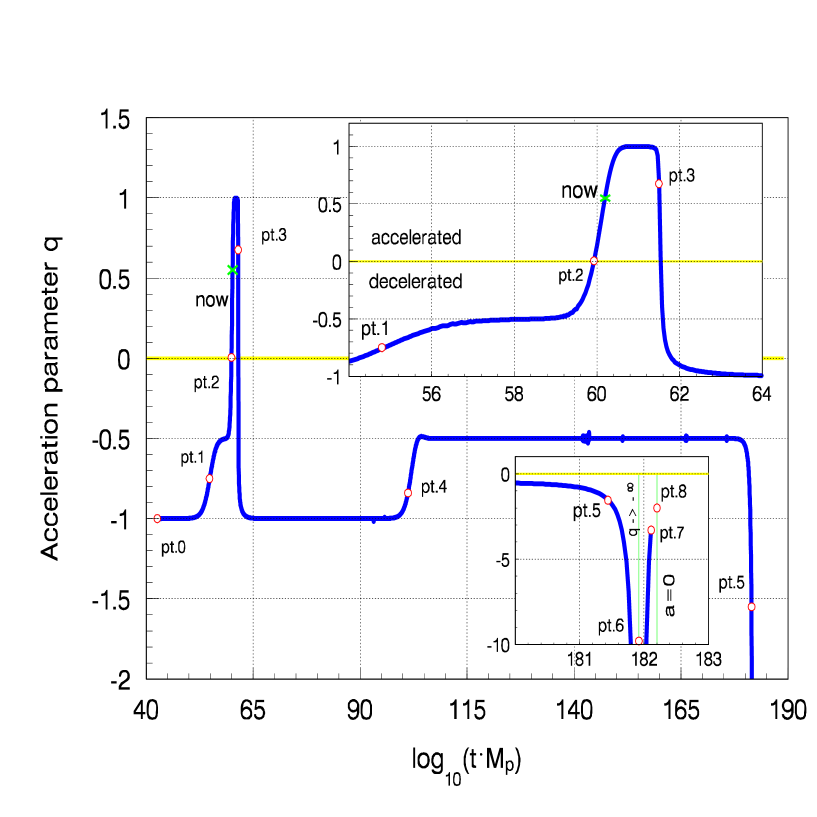
FIG. 1.:   The evolution of the acceleration parameter $q$ by computer simulation. The first stage is the radiation dominated from $t_{0}=0.4\times 10^{43}M_{p}^{-1}$ to $t_{1}=0.6\times 10^{55}M_{p}^{-1}$. The second stage is the matter dominated from $t_{1}$ to $t_{2}=0.86\times 10^{60}M_{p}^{-1}$. The third stage is the quintessence potential energy dominated from $t_{2}$ to $t_{3}=3.2\times 10^{61}M_{p}^{-1}$. The fourth stage is the quintessence kinetic energy dominated from $t_{3}$ to $t_{4}=1.6\times 10^{101}M_{p}^{-1}$. The fifth stage is the matter leading attractor from $t_{4}$ to $t_{5}=0.28\times 10^{182}M_{p}^{-1}$. The sixth stage is the curvature energy dominated from $t_{5}$ to $t_{6}=0.85\times 10^{182}M_{p}^{-1}$. The seventh stage is a big collapse with the quintessence kinetic energy dominated from $t_{6}$ to $t_{8}=1.74\times 10^{182}M_{p}^{-1}$. Specially, $t_{now}=t_{u}=1.56\times 10^{60}M_{p}^{-1}=13Gyr$.

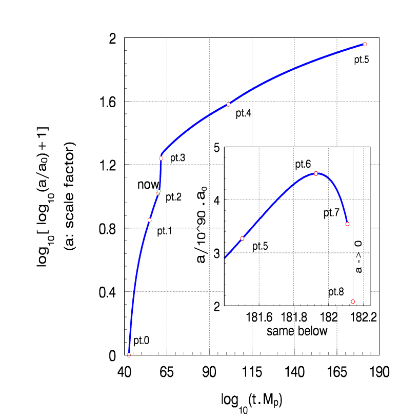
FIG. 2.:   The evolution of the cosmic scale factor $a$. Because its varying scope is too large, we have to use the double logarithm coordinates. In order to get a normalization, we add a minus one in it. You can see that the scale factor is shrinking in the stage 7. Some data are, $a_{1}=1.2\times 10^{6}a_{0}$, $a_{2}=2.4\times 10^{9}a_{0}$, $a_{now}=a_{u}=4\times 10^{9}a_{0}$, $a_{3}=1.7\times 10^{16}a_{0}$, $a_{4}=1.8\times 10^{37}a_{0}$, $a_{5}=3.1\times 10^{90}a_{0}$, $a_{6}=4.5\times 10^{90}a_{0}$, $a_{7}=0.27\times 10^{90}a_{0}$, and $a_{8}=0$.

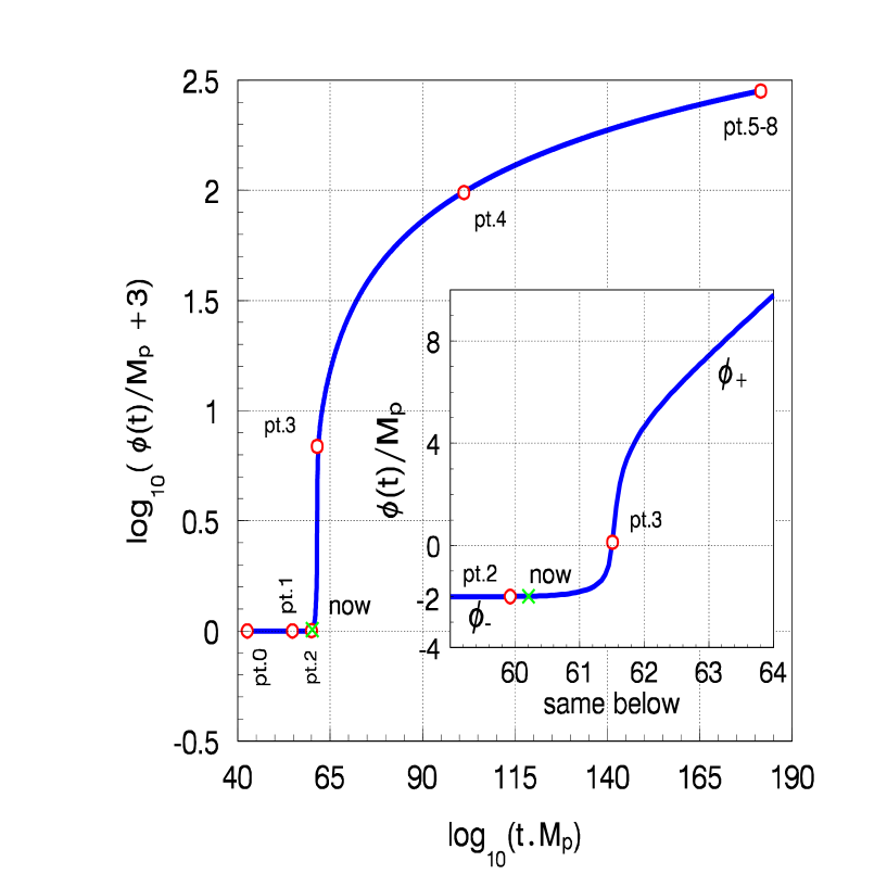
FIG. 3.:   The evolution of the quintessence field value $\phi$. In order to look at a detail of the behavior in small field value, we use the logarithm coordinates. In order to avoid singularity for iniyial value $-2$ , we have to add three in it. The curve is constructed by $\phi_{-}$ of Eq.(8) for $\phi<0$ and $\phi_{+}$ of Eq,(12) for $\phi>0$, there is a transition at time $t_{3}$. Some data are: $\phi_{0}=-2M_{p}$, $\phi_{1}=-2M_{p}$, $\phi_{2}=-1.997M_{p}$, $\phi_{3}=0.026M_{p}$, $\phi_{4}=95M_{p}$, $\phi_{5}=280M_{p}$, $\phi_{6}=281.5M_{p}$, and $\phi_{7}=289.1M_{p}$.

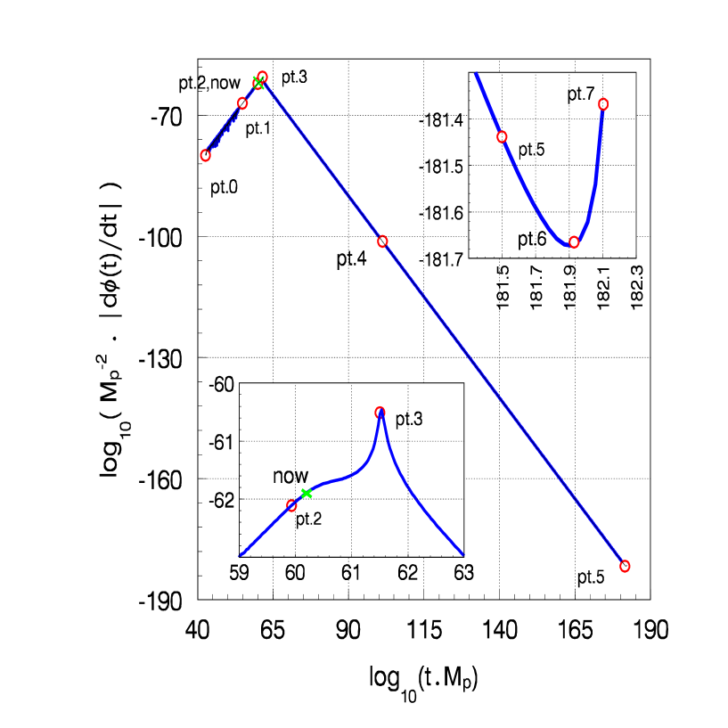
FIG. 4.:   The evolution of the velocity of the quintessence, $d\phi/dt$. This figure includes more information. You can magnify it in your computer to watch a detail for the main curve, specially, points $3$ and $5-8$. Some data are: $\dot{\phi}_{0}=0$, $\dot{\phi}_{1}=0.63\times 10^{-67}M_{p}^{2}$, $\dot{\phi}_{2}=0.8\times 10^{-62}M_{p}^{2}$, $\dot{\phi}_{3}=0.32\times 10^{-60}M_{p}^{2}$, $\dot{\phi}_{4}=0.63\times 10^{-101}M_{p}^{2}$, $\dot{\phi}_{5}=0.4\times 10^{-181}M_{p}^{2}$, $\dot{\phi}_{6}=0.21\times 10^{-181}M_{p}^{2}$, and $\dot{\phi}_{7}=10^{-178}M_{p}^{2}$. It is notable that the point 6 is not at the minimum of the curve, but is at its right side, therefore, $d^{2}\phi/dt^{2}>0$, see Eq.(16).