The Population of Weak Mgii Absorbers. II. The Properties of Single–Cloud Systems

Abstract

We present an investigation of Mgii absorbers characterized as single–cloud “weak systems” (defined by $W_{r}(2796)<0.3$ Å) at $z\sim 1$. We measured column densities and Doppler parameters for Mgii and Feii in $15$ systems found in HIRES/Keck spectra at $6.6$ km s^-1. Using these quantities and Civ, Ly$\alpha$ and Lyman limit absorption observed with the Faint Object Spectrograph on the Hubble Space Telescope (resolution $\sim 230$ km s^-1) we applied photoionization models to each system to constrain metallicities, densities, ionization conditions, and sizes.

We find that:

1) Single–cloud weak systems are optically thin in neutral hydrogen and may have their origins in a population of objects distinct from the optically thick strong Mgii absorbers, which are associated with bright galaxies.

2) Weak systems account for somewhere between 25% to 100% of the $z<1$ Ly$\alpha$ forest clouds in the range $10^{15.8}\leq N({\hbox{{\rm H}\kern 1.00006pt{\sc i}}})\leq 10^{16.8}$ cm^-2.

3) At least seven of 15 systems have two or more ionization phases of gas (multiphase medium). The first is the low–ionization, kinematically simple Mgii phase and the second is a high–ionization Civ phase which is usually either kinematically broadened or composed of multiple clouds spread over several tens of km s^-1. This higher ionization phase gives rise to the majority of the Ly$\alpha$ absorption strength (equivalent width), though it often accounts for a minor fraction of a system’s $N({\hbox{{\rm H}\kern 1.00006pt{\sc i}}})$.

4) We identify a subset of weak Mgii absorber, those with $\log N({\hbox{{\rm Fe}\kern 1.00006pt{\sc ii}}})/N({\hbox{{\rm Mg}\kern 1.00006pt{\sc ii}}})>-0.3$, which we term “iron–rich”. Though there are only three of these objects in our sample, their properties are the best constrained because of their relatively strong Feii detections and the sensitivity of the $N({\hbox{{\rm Fe}\kern 1.00006pt{\sc ii}}})/N({\hbox{{\rm Mg}\kern 1.00006pt{\sc ii}}})$ ratio. These clouds are not $\alpha$–group enhanced and are constrained to have sizes of $\sim 10$ pc. At that size, to produce the observed redshift path density, they would need to outnumber $L^{\ast}$ galaxies by approximately six orders of magnitude. The clouds with undetected iron do not have well–constrained sizes; we cannot infer whether they are enhanced in their $\alpha$–process elements.

We discuss these results and the implications that the weak Mgii systems with detected iron absorption require enrichment from Type Ia supernovae. Further, we address how star clusters or supernova remnants in dwarf galaxies might give rise to absorbers with the inferred properties. This would imply far larger numbers of such objects than are presently known, even locally. We compare the weak systems to the weak kinematic subsystems in strong Mgii absorbers and to Galactic high velocity clouds. Though weak systems could be high velocity clouds in small galaxy groups, their neutral hydrogen column densities are insufficient for them to be direct analogues of the Galactic high velocity clouds.

1 Introduction

Absorption lines from intervening galaxies in quasar (QSO) spectra provide a wealth of information about the physical conditions of gas in these galaxies. Since QSO absorption line spectroscopy offers unmatched sensitivity to high redshifts and low column densities, the technique can be used to follow the gas phase in galaxies over cosmic time, from primordial galaxies to the local universe.

The resonant Mgii $\lambda\lambda 2796,2803$ doublet has been used extensively to find low ionization QSO absorption systems (e.g. Lanzetta, Turnshek, & Wolfe (1987) and Steidel & Sargent (1992)). At $z\sim 1$, Mgii absorbers with rest frame equivalent widths, $W_{r}(2796)$, greater than $0.3$ Å are optically thick in neutral hydrogen; they are observed to give rise to Lyman limit breaks (Churchill et al., 2000a). Furthermore, these “strong” systems almost always arise within $40h^{-1}$ kpc of bright ($L\geq 0.05~{}L^{\ast}$), normal galaxies (Bergeron & Boissé, 1991; Steidel, Dickinson, & Persson, 1994; Steidel, 1995). The gas kinematics are consistent with material in the disks and extended halos of galaxies (Lanzetta & Bowen, 1992; Petitjean & Bergeron, 1990; Churchill et al., 1996; Charlton & Churchill, 1998; Churchill & Vogt, 2001).

The discovery of weak systems (those with $W_{r}(2796)<0.3$ Å) in high resolution HIRES/Keck spectra (Churchill et al. (1999); hereafter Paper I) necessitates a revision in the standard picture. Weak systems comprise $\sim 65$% of Mgii selected absorbers by number, yet only 4 out of 19 whose fields have been imaged have a $\gtrsim 0.05~{}L^{*}$ galaxy candidates within $\simeq 50h^{-1}$ kpc (C. Steidel, private communication, ). The large redshift path number density of weak systems relative to that of Lyman limit systems (LLSs) statistically indicates that, unlike strong absorbers, the majority of weak systems arise in optically thin neutral hydrogen (sub–Lyman limit) environments (see Figure 5 of Paper I). This has been observationally confirmed by Churchill et al. (2000a). Furthermore, the majority of weak systems are single clouds, often unresolved in HIRES/Keck spectra (resolution $6.6$ km s^-1), in striking contrast to the complex kinematics of strong Mgii absorbers (Petitjean & Bergeron, 1990; Churchill & Vogt, 2001). This evidence suggests that a substantial fraction of the weak Mgii systems selects a population of objects distinct from the bright, normal galaxies that are selected by the strong Mgii absorbers.

This begs the question: what are these single–cloud objects that outnumber Mgii–absorbing galaxies, yet often have no obvious luminous counterparts? A first strategy for addressing this question, adopted in this paper, is to constrain the column densities, metallicities, ionization conditions, and sizes of single–cloud weak systems.

Setting useful constraints on these physical conditions requires not just low ionization species, but also neutral hydrogen and medium to high ionization species. At $z\sim 1$, the Lyman series and the Cii, Civ, and Siiv transitions fall in the near ultraviolet (UV). These transitions were observed with the low–resolution Faint Object Spectrograph onboard the Hubble Space Telescope (FOS/HST). Churchill & Charlton (1999) have demonstrated that photoionization modeling using both high–resolution optical spectra and low–resolution UV spectra can yield meaningful constraints on the physical conditions of Mgii absorbers. We have adapted their approach to study weak systems.

In § 2 we describe the optical and UV spectra used in this study, and discuss sample selection to motivate our focus on single–cloud weak Mgii systems. In § 2.5, we describe our methods for Cloudy (Ferland, 1996) photoionization modeling to obtain constraints on cloud metallicities, ionization conditions, and sizes. The resulting constraints for the fifteen single–cloud weak Mgii systems are presented in § 3 and summarized in § 4. In § 5 we consider what types of astrophysical environments could be consistent with the properties of the weak single–cloud Mgii absorbers. In § 6 we speculate about the evolution of weak Mgii systems and suggest future investigations.

2 Data and Sample

2.1 The HIRES Spectra

Weak systems were charted in a survey of $26$ QSO spectra (Paper I) obtained with the HIRES spectrograph (Vogt et al., 1994) on the Keck I telescope. A total of 30 systems were found, with 22 of them being new discoveries. The survey covered the redshift interval $0.4\leq z\leq 1.4$, and was unbiased for $W_{r}(2796)<0.3$ Å. The spectral resolution was $R=45,000$ (fwhm = 6.6 km s^-1) with a typical signal–to–noise ratio of $S/N\simeq 30$ per three–pixel resolution element. The survey was $80$% complete for a $5\sigma$ equivalent width detection threshold of $W_{r}(2796)=0.02$ Å. We restrict our study to those systems with this limiting equivalent width in the continuum at the $\lambda 2796$ transition. Simulations reveal that Voigt profile fits to HIRES data become increasing less certain below this limit (Churchill, 1997; Churchill & Vogt, 2001). This equivalent width cutoff removes from this sample three systems from Paper I: S9, S11, and S22.

Data reduction, line identification, and Mgii doublet identification have been described in Paper I. In Figure 1 we display all the detected transitions (Mgii, Feii, and Mgi) associated with the $16$ weak single–cloud Mgii absorbers found in regions of the HIRES spectra that satisfy our equivalent width selection criterion.

2.2 Physically Motivated Sample

The adopted equivalent width demarcation at $W_{r}(2796)=0.3$ Å between “weak” and “strong” Mgii absorbers is an artifact of observational sensitivity (e.g. Steidel & Sargent (1992)). However, there are at least two physical conditions that set weak systems apart from strong systems. First, almost all weak systems are optically thin to neutral hydrogen. This was shown statistically in Paper I and observationally in Churchill et al. (2000a). By contrast, strong Mgii absorbers are Lyman limit systems, and thus by definition are optically thick in neutral hydrogen.

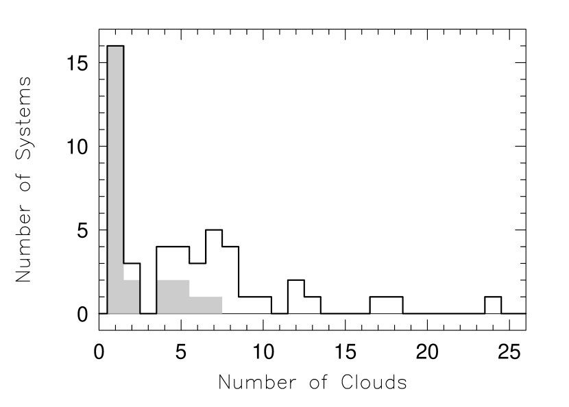
Second, the weak systems are often single clouds with very small velocity widths (unresolved in the HIRES spectra). For the sample of $30$ weak systems presented in Paper I, the number of clouds per weak system ranges from $1$ to $7$. Figure 2 shows the frequency distribution of the number of clouds per system for both the strong systems and the weak systems. The number of clouds per strong absorption system follows a Poissonian distribution with a median of $7$ clouds (see Table 7 of Churchill & Vogt (2001)). In contrast, the distribution for weak systems is non–Poissonian, with a spike at one cloud per absorber, i.e. there are many single–cloud weak systems. This suggests that these Mgii absorbers represent a distinct population of objects. To produce many more single–cloud absorbers than multiple–cloud absorbers, weak systems should have a small covering factor or a preferred large–scale geometry, such that a line of sight is unlikely to intersect multiple clouds.

In this paper we study the single–cloud systems. This selection criterion, together with the equivalent width cutoff described in § 2.1, yield $16$ single–cloud systems from the sample of $30$ systems of Paper I.

2.3 The FOS Spectra

For $13$ of the $16$ single–cloud systems, archival FOS/HST spectra were available. The resolution of these spectra was $\sim 230$ km s^-1 fwhm, with four diodes per resolution element. For PKS $0454+039$ and PKS $0823-223$, which contain three single–cloud weak systems, the spectra were retrieved from the archive and reduced in collaboration with S. Kirhakos, B. Jannuzi, and D. Schneider (Churchill et al., 2000a), using the techniques and software of the HST QSO Absorption Line Key Project (Schneider et al., 1993). The remaining six QSOs were observed and published by the Key Project (Bahcall et al., 1993, 1996; Jannuzi et al., 1998) and have kindly been made available for this work. Further details of the FOS/HST observations and the analysis were presented in Churchill et al. (2000a). In general, for the single–cloud weak systems discussed here, the useful FOS transitions were Civ, Ly$\alpha$, and the Lyman limit, since they are strong features commonly covered in the archive data. Table The Population of Weak Mgii Absorbers. II. The Properties of Single–Cloud Systems lists the equivalent widths and limits for Civ and Ly$\alpha$, taken from Churchill et al. (2000a).

In Figure 3, spectra covering Mgii, Feii, Civ, Ly$\alpha$ and the Lyman limit are displayed for each system to show, in a single view, the full sample including blends, non–detections, and non–coverage. Additional transitions observed in the FOS data but not plotted in Figure 3 can be found in Churchill et al. (2000a).

2.4 Column Densities

For the HIRES spectra, the column densities and Doppler parameters were obtained using Minfit, a $\chi^{2}$ minimization Voigt profile fitter (Churchill, 1997; Churchill & Vogt, 2001; Churchill, Vogt, & Charlton, 2001). The column densities and Doppler parameters of the fits to Mgii and Feii are listed in Table The Population of Weak Mgii Absorbers. II. The Properties of Single–Cloud Systems , as are $3\sigma$ upper limits on the Feii column density for cases where no Feii transitions were detection. The latter were obtained from the $3\sigma$ equivalent width limit for Feii $\lambda 2600$, assuming a Doppler parameter equal to that obtained for Mgii in the same system.

The column density ratio, $N({\hbox{{\rm Fe}\kern 1.00006pt{\sc ii}}})/N({\hbox{{\rm Mg}\kern 1.00006pt{\sc ii}}})$, is critically important to the photionization modeling; as discussed in § 2.5.1, this ratio constrains the ionization parameter. Therefore, it is important to appreciate the systematic errors when $N({\hbox{{\rm Mg}\kern 1.00006pt{\sc ii}}})$ and $N({\hbox{{\rm Fe}\kern 1.00006pt{\sc ii}}})$ are comparable in strength. Simulations reveal that a $5\sigma$ equivalent width detection limit of $0.02$ Å in HIRES spectra gives a 99% completeness limit of $\log N({\hbox{{\rm Mg}\kern 1.00006pt{\sc ii}}})=11.9$ cm^-2 and $\log N({\hbox{{\rm Fe}\kern 1.00006pt{\sc ii}}})=12.4$ cm^-2 (Churchill, 1997; Churchill, Vogt, & Charlton, 2001). Above these column densities Minfit accurately models the column densities. For $\log N({\hbox{{\rm Fe}\kern 1.00006pt{\sc ii}}})<12.4$ cm^-2, Minfit statistically overestimates $\log N({\hbox{{\rm Fe}\kern 1.00006pt{\sc ii}}})$ by up to $\sim 0.3$ dex (Churchill (1997), Figure 4.8) due to a bias toward “false detections” in “favorable” noise patterns. Mgii Doppler parameters were well recovered in the simulations, with an RMS scatter of $\sim 1$ km s^-1 for all column densities above the sensitivity cutoff. Feii Doppler parameters were poorly recovered when the column density was near or below the sensitivity cutoff (Churchill, 1997).

For an Feii detection at the $3\sigma$ level in the lowest $S/N$ spectrum in our sample, the detection limit (99% completeness) for the ratio $N({\hbox{{\rm Fe}\kern 1.00006pt{\sc ii}}})/N({\hbox{{\rm Mg}\kern 1.00006pt{\sc ii}}})$ would be

$$\log[N({\hbox{{\rm Fe}\kern 1.00006pt{\sc ii}}})/N({\hbox{{\rm Mg}\kern 1.00006pt{\sc ii}}})]=12.2-\log N({\hbox{{\rm Mg}\kern 1.00006pt{\sc ii}}}),$$ (1)

Therefore, with increasing $N({\hbox{{\rm Mg}\kern 1.00006pt{\sc ii}}})$ the upper limit on $N({\hbox{{\rm Fe}\kern 1.00006pt{\sc ii}}})/N({\hbox{{\rm Mg}\kern 1.00006pt{\sc ii}}})$ decreases, i.e. becomes more stringent. We show this relation in Figure 4 as a diagonal line. The value of $\log N({\hbox{{\rm Fe}\kern 1.00006pt{\sc ii}}})/N({\hbox{{\rm Mg}\kern 1.00006pt{\sc ii}}})$ for each of the single–cloud weak systems is plotted, with detections as solid circles and upper limits as downward–pointing arrows. Note that since the plotted $N({\hbox{{\rm Fe}\kern 1.00006pt{\sc ii}}})/N({\hbox{{\rm Mg}\kern 1.00006pt{\sc ii}}})$ detection limit line was computed from the noisiest spectrum in our sample, the data points are often lower than the limit, and thus are more constraining of the Feii to Mgii ratio than the line indicates.

Since there is an apparent gap in the distribution of $\log N({\hbox{{\rm Fe}\kern 1.00006pt{\sc ii}}})/N({\hbox{{\rm Mg}\kern 1.00006pt{\sc ii}}})$, we somewhat arbitrarily define systems with detectable Feii and $\log N({\hbox{{\rm Fe}\kern 1.00006pt{\sc ii}}})/N({\hbox{{\rm Mg}\kern 1.00006pt{\sc ii}}})>-0.3$ (systems S7, S13, and S18) as “iron–rich” weak systems.

Since all three so–called “iron–rich” systems lie above the worst–case sensitivity line, and all other systems fall below it, there may be a selection effect at work – are the highest $N({\hbox{{\rm Mg}\kern 1.00006pt{\sc ii}}})$ systems identified as “iron–rich” systems simply because their Feii is easier to detect? We argue that this is not the case. To illustrate, we consider the five systems with $N({\hbox{{\rm Mg}\kern 1.00006pt{\sc ii}}})$ between that of S18 and S7 (two iron–rich systems.) If these five systems had $\log N({\hbox{{\rm Fe}\kern 1.00006pt{\sc ii}}})/N({\hbox{{\rm Mg}\kern 1.00006pt{\sc ii}}})\sim~{}0$, as is true for the iron–rich systems, then Figure 4 makes clear that they should have detected Feii. Only one of the five systems does (S28), and since it has $\log N({\hbox{{\rm Fe}\kern 1.00006pt{\sc ii}}})/N({\hbox{{\rm Mg}\kern 1.00006pt{\sc ii}}})\simeq-0.6$, it is not deemed iron–rich. The limits on $\log N({\hbox{{\rm Fe}\kern 1.00006pt{\sc ii}}})/N({\hbox{{\rm Mg}\kern 1.00006pt{\sc ii}}})$ for the other four systems are also well below $0$, by more than half a dex. Thus, it seems that while we have insufficient information to address whether the distribution of $N({\hbox{{\rm Fe}\kern 1.00006pt{\sc ii}}})/N({\hbox{{\rm Mg}\kern 1.00006pt{\sc ii}}})$ is continuous or bimodal, the iron–rich systems do appear to have significantly higher $N({\hbox{{\rm Fe}\kern 1.00006pt{\sc ii}}})$ to $N({\hbox{{\rm Mg}\kern 1.00006pt{\sc ii}}})$ ratios than do the other systems. As § 2.5.1 will show, this difference in column density ratios indicates variations in ionization and/or abundance pattern between the “iron–rich” systems and the other systems.

2.5 Photoionization Modeling

We assume that the single–cloud, weak systems are in photoionization equilibrium and constrain their properties with the photoionization code Cloudy, version 90.4 (Ferland, 1996). The clouds are modeled as constant density, plane–parallel slabs and are matched to the Mgii and Feii column densities measured from the HIRES spectra. Using each model’s output column densities for ions of interest, we synthesized FOS/HST spectra, which we directly compared to the observed Civ and Ly$\alpha$ profiles and to the spectral region covering the Lyman limit break. This procedure constrains both the ionization conditions and gas–phase metallicities. Further discussion of the modeling technique was presented by Churchill & Charlton (1999) and by Charlton et al. (2000).

We begin each analysis with the assumption that the Mgii, Feii, Ly$\alpha$, and Civ arise in a single isothermal structure, described by a single metallicity and ionization parameter. The data often show that this assumption is violated, in which case we model two phases, each having its own metallicity, temperature, and ionization parameter. Further details are presented below.

Clouds were assumed to be ionized by a Haardt & Madau background spectrum (Haardt & Madau, 1996). For cloud redshifts below $z=0.75$, we used a spectrum shape and normalization at $z=0.5$ and for redshifts above $z=0.75$ we used the shape and normalization at $z=1.0$. For all models, we assumed a solar abundance pattern. In § 2.5.5, we discuss possible abundance pattern variations and the effect of alternative spectral shapes.

2.5.1 Applying Constraints to the Mgii Cloud

As Figure 5 illustrates, when the assumption of photoionization equilibrium holds, the $N({\hbox{{\rm Fe}\kern 1.00006pt{\sc ii}}})/N({\hbox{{\rm Mg}\kern 1.00006pt{\sc ii}}})$ and $N({\hbox{{\rm C}\kern 1.00006pt{\sc iv}}})/N({\hbox{{\rm Mg}\kern 1.00006pt{\sc ii}}})$ ratios are uniquely determined by the ionization parameter, which is defined as $U=n_{\gamma}/n_{\rm H}$, where $n_{\gamma}$ and $n_{\rm H}$ are the number density of photons capable of ionizing hydrogen and the total hydrogen number density, respectively. Therefore, $\log U=\log n_{\gamma}-\log n_{\rm H}$, where $n_{\gamma}$ is set by the background spectrum. For the Haardt & Madau (1996) spectrum, $\log n_{\gamma}=-5.6$ at $z=0.5$ and $\log n_{\gamma}=-5.2$ at $z=1.0$.

When $N({\hbox{{\rm Mg}\kern 1.00006pt{\sc ii}}})$ and $N({\hbox{{\rm Fe}\kern 1.00006pt{\sc ii}}})$ were both measured, they were used to constrain the optimized mode of Cloudy at a set metallicity to yield $U$ and $N({\hbox{{\rm H}\kern 1.00006pt{\sc i}}})$ by varying both $N({\hbox{{\rm H}\kern 1.00006pt{\sc i}}})$ and $n_{\rm H}$. Models were run for a range of metallicities, $-2.5\leq Z\leq 0$, in increments of $0.5$ dex.

When only an upper limit on $N({\hbox{{\rm Fe}\kern 1.00006pt{\sc ii}}})$ was measured, we created a grid of Cloudy models over $\log U$ (from $-2$ to $-5$, in $0.1$ dex intervals) and $Z$ (from $0$ to $-2.5$, in $0.5$ dex intervals.) $N({\hbox{{\rm Mg}\kern 1.00006pt{\sc ii}}})$ provided the constraint, and $N({\hbox{{\rm H}\kern 1.00006pt{\sc i}}})$ was the parameter for which Cloudy solved. We rejected ionization parameters whose models, over the whole metallicity range, yielded $N({\hbox{{\rm Fe}\kern 1.00006pt{\sc ii}}})$ that was greater than the $3\sigma$ limits listed in Table 1. This set lower limits on the ionization parameter.

A model was judged to have failed or be inapplicable for any of the following three reasons: failure to converge upon an ionization parameter (usually when $N({\hbox{{\rm Fe}\kern 1.00006pt{\sc ii}}})/N({\hbox{{\rm Mg}\kern 1.00006pt{\sc ii}}})\simeq 1$); cloud size exceeded the Jeans’ length and was thus unstable to collapse; cloud size exceeded $50$ kpc.

2.5.2 Metallicities and Multiple Ionization Phases

Whereas the ionization parameter is constrained by the Mgii and Feii HIRES data, the metallicity and $N({\hbox{{\rm H}\kern 1.00006pt{\sc i}}})$ are constrained by the Ly$\alpha$ profiles and presence or absence of the Lyman limit break in the FOS spectra. In the regime where a cloud is optically thin at the Lyman limit, to create more $W_{r}({\hbox{{\rm Ly}\kern 1.00006pt$\alpha$}})$, given a measured $N({\hbox{{\rm Mg}\kern 1.00006pt{\sc ii}}})$, requires lowering the metallicity, which increases $N({\hbox{{\rm H}\kern 1.00006pt{\sc i}}})$ the total hydrogen column density $N_{\rm H}$, where $N_{\rm H}=N({\hbox{{\rm H}\kern 1.00006pt{\sc i}}})+N({\hbox{{\rm H}\kern 1.00006pt{\sc ii}}})$, and the cloud size.

Because the low-resolution FOS/HST profiles are largely dominated by the instrumental spread function, their column densities and Doppler parameters cannot be directly measured. In order to use the FOS spectra as a constraint, we created synthetic FOS spectra (infinite sampling and signal–to–noise ratio) using the kinetic temperature and column densities output by Cloudy.

First, we assumed a priori that all detected absorption arises in one phase of gas, the same phase that gives rise to Mgii absorption. Using the temperature of the Cloudy model and the measured $b({\hbox{{\rm Mg}\kern 1.00006pt{\sc ii}}})$, we solved for the turbulent component, $b_{turb}$, and computed the Doppler parameter for other ions by the relation

$$b_{ion}^{2}=2kT/m_{ion}+b_{turb}^{2}.$$ (2)

This inferred Doppler parameter and the column density are used to generate a Voigt profile, which is then convolved with the FOS instrumental spread function to produce a synthesized spectral feature.

To constrain each cloud’s metallicity, we visually compared the synthesized and FOS Ly$\alpha$ profiles for each modeled metallicity. In Figure 6, we illustrate the metallicity fitting procedure. Metallicities of $Z=0$, $-1$, $-2$, and $-2.5$ are plotted; clearly, $Z=0$ and $Z=-1$ do not fit the Ly$\alpha$ profile nor are their equivalent widths consistent with the measured value, and $Z=-2.5$ slightly overpredicts the Ly$\alpha$ absorption. In this example, assuming a single phase produces the Ly$\alpha$ absorption, the metallicity is constrained to be in the range $-2.5<Z<-1$.

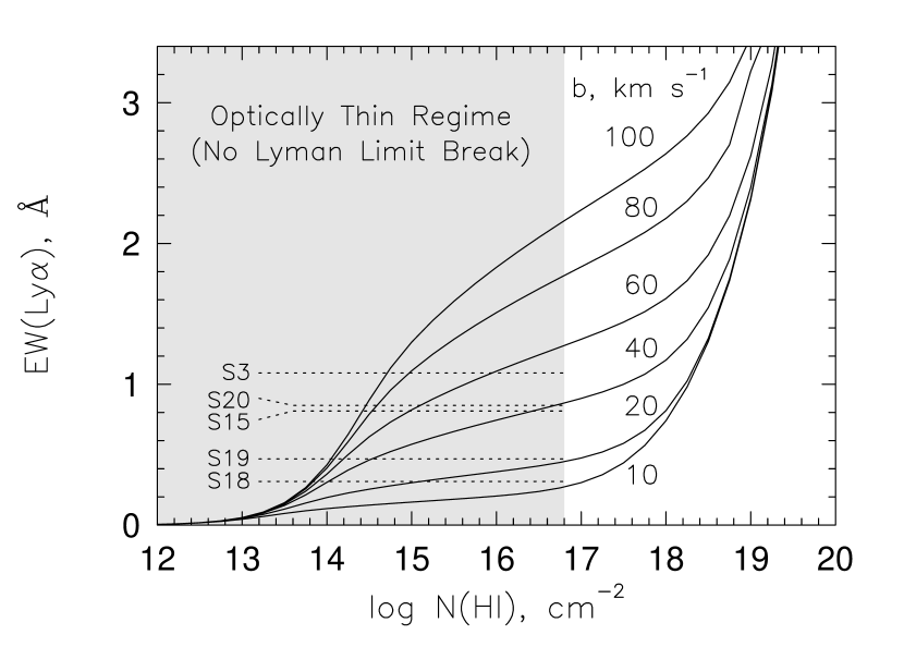
For the systems for which the Lyman limit break is known to be absent, an additional metallicity constraint may be imposed. From the Ly$\alpha$ curve of growth, shown in Figure 7, for a given $N({\hbox{{\rm H}\kern 1.00006pt{\sc i}}})$ we can find the $b({\hbox{{\rm H}\kern 1.00006pt{\sc i}}})$ required to observe a given $W({\hbox{{\rm Ly}\kern 1.00006pt$\alpha$}})$. The lack of a Lyman limit break provides a direct constraint, $\log N({\hbox{{\rm H}\kern 1.00006pt{\sc i}}})<16.8$ cm^-2, which then implies a lower limit on $b({\hbox{{\rm H}\kern 1.00006pt{\sc i}}})$. If this $b({\hbox{{\rm H}\kern 1.00006pt{\sc i}}})$ is larger than that implied by thermal scaling of $b({\hbox{{\rm Mg}\kern 1.00006pt{\sc ii}}})$ for the cloud, then there is evidence for a second phase of gas. Much of the Ly$\alpha$ equivalent width must arise in this second phase, whose larger Doppler parameter produces the observed $W_{r}({\hbox{{\rm Ly}\kern 1.00006pt$\alpha$}})$ without exceeding the limit on $N({\hbox{{\rm H}\kern 1.00006pt{\sc i}}})$ (imposed by the Lyman limit). With such a second phase present, the $N({\hbox{{\rm H}\kern 1.00006pt{\sc i}}})$ would be smaller in the Mgii cloud phase, and the metallicity “constraint” should be taken as a lower limit.

The strength of the Ly$\alpha$ profile depends only weakly on the ionization parameter for most of the range under consideration. Accordingly, when the ionization parameter was poorly constrained, we constrained the metallicity at the low and high ends of the permitted $U$ range, so that the quoted metallicity constraint holds for the range of possible ionization parameters.

2.5.3 Multiple Ionization Phases Required by Civ

Often, the single–phase Mgii cloud model could not account for the observed Civ strength, even for the highest possible ionization parameter. If Feii is detected, it imposes a strict upper limit on the ionization parameter, and therefore on $N({\hbox{{\rm C}\kern 1.00006pt{\sc iv}}})$. If Feii is not detected, a high ionization parameter and therefore a large $N({\hbox{{\rm C}\kern 1.00006pt{\sc iv}}})$ is possible. However, with a small $b({\hbox{{\rm C}\kern 1.00006pt{\sc iv}}})$, scaled from the measured $b({\hbox{{\rm Mg}\kern 1.00006pt{\sc ii}}})$, it may still not be possible for the model to reproduce the observed $W_{r}({\hbox{{\rm C}\kern 1.00006pt{\sc iv}}})$. Single–phase models were rejected when the equivalent widths of the synthesized profiles fell at least $3\sigma$ below that measured in the FOS data; a second phase with a larger $b({\hbox{{\rm C}\kern 1.00006pt{\sc iv}}})$ was then required. This second phase should be sufficiently ionized that it does not produce a detectable broad Mgii component. However, its other properties (eg. its Doppler parameter and metallicity) are not well constrained by the low resolution FOS spectrum.

The Civ $\lambda\lambda 1548,1550$ doublet ratio can also indicate that Civ absorption occurs in a broader phase. If all transitions arose in the narrow Mgii phase, the Civ doublet would be saturated and unresolved, with a doublet ratio of $\sim 1$. By contrast, a broad phase would produce less saturated lines, and a Civ doublet ratio closer to the natural value of $2$. This argument is not model–dependent but relies only on the spectral resolution of FOS/HST. Unfortunately, the errors in the doublet ratio are large; S17 is the only system for which the doublet ratio can be used to infer that the Civ arises in a broader phase than the Mgii.

2.5.4 Inferred Sizes and Masses

The derived cloud size (plane parallel thickness) is simply $d=N_{\rm H}/n_{\rm H}$, where $N_{\rm H}$ is the total hydrogen column density, $N({\hbox{{\rm H}\kern 1.00006pt{\sc i}}})+N({\hbox{{\rm H}\kern 1.00006pt{\sc ii}}})$. Assuming a spherical geometry, we can estimate the cloud masses within a geometric factor as

$$M_{cl}\simeq 4~{}\bigg{(}\frac{N_{\rm H}}{10^{18}~{}{\rm cm}^{-2}}\bigg{)}^{3}\bigg{(}\frac{10^{-2}~{}{\rm cm}^{-3}}{n_{\rm H}}\bigg{)}^{2}\quad{\rm M}_{\odot}.$$ (3)

Because $n_{\rm H}=n_{\gamma}/U$, this equation can also be written in terms of the ionization parameter where $n_{\gamma}$ is slightly redshift dependent.

2.5.5 Robustness to Assumptions

Much of what can be inferred and/or deduced about the physical and cosmological properties of single–cloud weak systems is directly related to the size and mass measurements from the models. Here, we examine the sensitivity of these quantities to our modeling assumptions.

First, we have assumed photoionization equilibrium. Photoionization models have been shown to underestimate the sizes of some Ly$\alpha$ forest clouds by several orders of magnitude (Haehnelt, Rauch, & Steinmetz, 1996). In these cases, the gas is not in full thermal equilibrium because of additional heating from shocks, and errors in temperature propagate to large errors in derived size. Such non–equilibrium is found to occur for $\log n_{\rm H}\leq-4$ cm^-3, corresponding to the high ionization conditions of higher redshift Ly$\alpha$ forest clouds, where recombination timescales can rival a Hubble time. At $z=1$, such a density corresponds to $\log U=-1.4$. As shown in Figure 5, photoionized clouds with $N({\hbox{{\rm Fe}\kern 1.00006pt{\sc ii}}})\simeq N({\hbox{{\rm Mg}\kern 1.00006pt{\sc ii}}})$ are constrained to have $\log U\leq-3.5$. Thus, iron–rich weak Mgii systems have densities too high, or equivalently ionization parameters too low, for their sizes to be underestimated in this manner.

Second, we have assumed that the gas is ionized by a Haardt & Madau (1996) extragalactic UV background spectrum. Since high luminosity counterparts are apparently rarely associated with weak systems, the most likely stellar contribution to the spectrum would be that from a single star or small group of stars quite near to the cloud. However, the constraints on the stellar types, number of stars and their distance from the cloud can be quite severe (e.g. Churchill & Le Brun (1998), Appendix B). To explore model sensitivity to the spectral shape, we produced a Cloudy grid, similar to that in Figure 5, for a stellar spectrum characteristic of $T=30,000$ K stars. Such a spectrum, though it is too soft to ionize carbon into Civ, still has Feii/Mgii that decreases with increasing ionization parameter. Thus a low ionization parameter (and high density) is still required for the Mgii clouds, especially those with measured Feii.

Third, we have assumed a solar abundance pattern with no depletion onto dust grains. Enhancement of $\alpha$–process elements relative to iron would shift the Cloudy grid in Figure 4 down, so that a given $N({\hbox{{\rm Fe}\kern 1.00006pt{\sc ii}}})/N({\hbox{{\rm Mg}\kern 1.00006pt{\sc ii}}})$ ratio would correspond to a lower ionization parameter and smaller cloud size. By contrast, iron enhancement would make the clouds larger than we infer, but such enhancement is rarely found in astrophysical environments (Edvardsson et al., 1993; McWilliam, 1997). Dust depletion would mimic $\alpha$ enhancement, since iron depletes more readily than magnesium by as much as 0.5 dex (e.g. Lauroesch et al. (1996) and Savage & Sembach (1996a)). Dust would also affect the cooling function in the models. To investigate model sensitivity to this, we ran Cloudy models for S7 (a high $N({\hbox{{\rm Fe}\kern 1.00006pt{\sc ii}}})/N({\hbox{{\rm Mg}\kern 1.00006pt{\sc ii}}})$ system) both with no dust and with varying amounts of dust scaled relative to the ISM level (taken from the Cloudy database). Dust had a negligible effect on cloud sizes for dust abundances up to ten times ISM. At higher levels, the cloud sizes decreased with increasing dust content.

To summarize, the model cloud properties are robust to the modeling assumptions. In particular, the conclusion seems robust that clouds with $N({\hbox{{\rm Fe}\kern 1.00006pt{\sc ii}}})\simeq N({\hbox{{\rm Mg}\kern 1.00006pt{\sc ii}}})$ and low $N({\hbox{{\rm H}\kern 1.00006pt{\sc i}}})$ are small. If some unknown effect has led us to underestimate the cloud sizes of the iron–rich clouds by $2$–$3$ orders of magnitude, then the discussion of their origins in §5.4.1 does not apply, and the discussion in §5.4.2 for clouds with lower $N({\hbox{{\rm Fe}\kern 1.00006pt{\sc ii}}})/N({\hbox{{\rm Mg}\kern 1.00006pt{\sc ii}}})$ would be more suitable.

3 Individual System Properties

For each single–cloud weak system, we first summarize in brackets the coverage and detection status of Feii, Ly$\alpha$, the Lyman limit, and Civ. We then explain the constraints these transitions impose. Lastly, in brackets we summarize the evidence or lack of evidence for multiple phases of gas. Systems are listed in redshift order, with system numbers adopted from Paper I. The constraints for all systems are summarized in Table The Population of Weak Mgii Absorbers. II. The Properties of Single–Cloud Systems .

3.1 S1 (Q$1421+331$; $z_{\rm abs}=0.45642$)

[Feii not covered; no FOS spectra.] Since Ly$\alpha$ and the Lyman limit were not covered, the metallicity of this system cannot be constrained. The ionization parameter cannot be constrained because Feii and Civ were not covered. We do not include this system in discussions of multiple phases and Feii statistics because of the lack of spectral coverage. [Cannot address multiphase.]

3.2 S3 (Q$1354+195$; $z_{\rm abs}=0.52149$)

[$N({\hbox{{\rm Fe}\kern 1.00006pt{\sc ii}}})$ upper limit; $W_{r}({\hbox{{\rm Ly}\kern 1.00006pt$\alpha$}})$ measured; no break at Lyman limit; $W_{r}({\hbox{{\rm C}\kern 1.00006pt{\sc iv}}})$ upper limit.] To produce the strong Ly$\alpha$ detection in this cloud requires $Z<-2.5$, assuming that all the Ly$\alpha$ absorption arises in the same phase of gas as the detected Mgii. However, the lack of a Lyman limit break requires $\log N({\hbox{{\rm H}\kern 1.00006pt{\sc i}}})<16.8$ cm^-2, which corresponds to $Z>-1.5$ for this cloud. Therefore, S3 possesses a second phase of gas with a larger Doppler parameter than that of the Mgii phase, which can produce the observed Ly$\alpha$ equivalent width without exceeding the Hi column density limit imposed by the Lyman limit. Feii and Civ limits do not constrain $U$. [Multiphase required because of Hi; Civ does not require or rule out multiphase.]

3.3 S6 (Q$0002+051$; $z_{\rm abs}=0.59149$)

[$N({\hbox{{\rm Fe}\kern 1.00006pt{\sc ii}}})$ upper limit; Ly$\alpha$ in spectropolarimetry mode; Lyman limit not covered; $W_{r}({\hbox{{\rm C}\kern 1.00006pt{\sc iv}}})$ upper limit.] The Ly$\alpha$ spectrum is not usable because it was taken in spectropolarimetry mode (Churchill et al., 2000a). This, combined with the lack of Lyman limit coverage, allows no constraints on metallicity. The Feii limit sets a fairly high lower limit on the ionization parameter: $\log U>-3.5$. The Civ limit is too poor to restrict the ionization parameter. [Cannot address multiphase.]

3.4 S7 (Q$0454+039$; $z_{\rm abs}=0.64283$)

[$N({\hbox{{\rm Fe}\kern 1.00006pt{\sc ii}}})$ measured; $W_{r}({\hbox{{\rm Ly}\kern 1.00006pt$\alpha$}})$ measured; Lyman limit not covered; $W_{r}({\hbox{{\rm C}\kern 1.00006pt{\sc iv}}})$ measured.] If we assume the Ly$\alpha$ arises in the Mgii phase, then to match the Ly$\alpha$ profile requires $-1<Z<0$. [This constraint differs somewhat from Churchill & Le Brun (1998) who used a different version of the FOS/HST spectrum.] Mgii and Feii constrain the ionization parameter to $-4.5<\log U<-3.6$ for the full range of metallicities modeled, and to $-4.5<\log U<-4.2$ for the metallicity range determined above. The model thicknesses range from $2$ pc for $Z=0$ to $8$ pc for $Z=-1$. If the cloud were enhanced in iron, both size and ionization parameter would increase. The large Feii/Mgii ratio requires a low ionization cloud which cannot produce the observed Civ or Siiv; a second phase of higher–ionization gas is required. [Multiphase is not required for Hi, but is required to explain Civ and Siiv.]

3.5 S8 (Q$0823-223$; $z_{\rm abs}=0.705472$)

[$N({\hbox{{\rm Fe}\kern 1.00006pt{\sc ii}}})$ upper limit; Ly$\alpha$ and Lyman limit not covered; $W_{r}({\hbox{{\rm C}\kern 1.00006pt{\sc iv}}})$ upper limit.] Neither Ly$\alpha$ nor the Lyman limit were covered, providing no metallicity constraint. The Feii and Civ limits set lower and upper limits, respectively, on the ionization parameter: $-3.6<\log U<-2.4$. In order not to exceed the $3\sigma$ equivalent width, $\log N({\hbox{{\rm C}\kern 1.00006pt{\sc iv}}})<14$ cm^-2. [Hi cannot address multiphase; Civ is consistent with a single phase.]

3.6 S12 (Q$1634+706$; $z_{\rm abs}=0.81816$)

[$N({\hbox{{\rm Fe}\kern 1.00006pt{\sc ii}}})$ upper limit; $W_{r}({\hbox{{\rm Ly}\kern 1.00006pt$\alpha$}})$ poor upper limit; Lyman limit not covered; $W_{r}({\hbox{{\rm C}\kern 1.00006pt{\sc iv}}})$ upper limit.] The available Ly$\alpha$ coverage is pre–COSTAR and in spectropolarimetry mode, and therefore unusable (Churchill et al., 2000a); accordingly, the metallicity of this system cannot be constrained. The Feii limit requires $\log U>-4.4$. The $3\sigma$ Civ limit, which sets $\log N({\hbox{{\rm C}\kern 1.00006pt{\sc iv}}})<15$ cm^-2, does not restrict $U$. [Hi cannot address multiphase; Civ is consistent with a single phase.]

3.7 S13 (Q$1421+331$; $z_{\rm abs}=0.84325$)

[$N({\hbox{{\rm Fe}\kern 1.00006pt{\sc ii}}})$ measured; no FOS spectra.] Without FOS spectra for this quasar, the metallicity cannot be constrained. $N({\hbox{{\rm Fe}\kern 1.00006pt{\sc ii}}})/N({\hbox{{\rm Mg}\kern 1.00006pt{\sc ii}}})$ is greater than unity for this cloud: $\log N({\hbox{{\rm Fe}\kern 1.00006pt{\sc ii}}})=13.47\pm 0.07$ cm^-2 and $\log N({\hbox{{\rm Mg}\kern 1.00006pt{\sc ii}}})=13.1\pm 0.1$ cm^-2. As Figures 4 and 5 demonstrate, this cannot occur for a solar abundance pattern and a Haardt & Madau (1996) ionizing background. The iron fit is particularly robust because five Feii transitions were detected at relatively high $S/N$. Unresolved saturation may be present in the Feii transitions, which would cause the fit to underestimate $N({\hbox{{\rm Fe}\kern 1.00006pt{\sc ii}}})$. If the Mgii doublet does not have unresolved saturation, then it could be that this cloud is iron enhanced, as depletion cannot yield this pattern. A model with iron enhanced by $0.5$ dex predicts $\log U=-4.3$ and cloud size from $1$–$12$ pc. [Without FOS spectra, multiphase cannot be addressed.]

3.8 S15 (Q$0002+051$; $z_{\rm abs}=0.86653$)

[$N({\hbox{{\rm Fe}\kern 1.00006pt{\sc ii}}})$ upper limit; $W_{r}({\hbox{{\rm Ly}\kern 1.00006pt$\alpha$}})$ measured; no break at Lyman limit; $W_{r}({\hbox{{\rm C}\kern 1.00006pt{\sc iv}}})$ upper limit.] If the observed Ly$\alpha$ absorption were produced in the Mgii cloud, this would require a cloud metallicity of $-2.5\leq Z\leq-2.0$, which corresponds to $18<\log N({\hbox{{\rm H}\kern 1.00006pt{\sc i}}})<20$ cm^-2. However, the small Doppler parameter of the Mgii cloud predicts an unresolved Ly$\alpha$ narrower than observed, and the lack of a break at the Lyman limit requires $\log N({\hbox{{\rm H}\kern 1.00006pt{\sc i}}})\leq 16.8$ cm^-2 and $Z>-1$ for all ionization parameters. Hence, much of the Ly$\alpha$ absorption arises not in the Mgii cloud, but in a separate phase of gas with a larger Doppler parameter (see Figure 7). The Feii limit constrains $\log U>-3.6$ in the Mgii cloud. Models can be made to meet but not exceed the Civ limit; therefore it does not constrain the ionization parameter; $\log N({\hbox{{\rm C}\kern 1.00006pt{\sc iv}}})<16.5$ cm^-2 could exist in the Mgii cloud. [Multiphase is inferred from Hi, though Civ does not require a second phase.]

3.9 S16 (Q$1241+176$; $z_{\rm abs}=0.89549$)

[$N({\hbox{{\rm Fe}\kern 1.00006pt{\sc ii}}})$ upper limit; $W_{r}({\hbox{{\rm Ly}\kern 1.00006pt$\alpha$}})$ measured; Lyman limit not covered; $W_{r}({\hbox{{\rm C}\kern 1.00006pt{\sc iv}}})$ upper limit.] If the Ly$\alpha$ and Mgii absorption arose in the same phase, then Ly$\alpha$ would be best fit by $-2.5<Z<-1$ (see Figure 6). The ionization parameter is constrained as $-4.8<\log U<-2.0$ by Feii and Civ limits. The upper limit of $N({\hbox{{\rm C}\kern 1.00006pt{\sc iv}}})$ from the $3\sigma$ equivalent width limit, $\log N({\hbox{{\rm C}\kern 1.00006pt{\sc iv}}})<13.4$ cm^-2, can be produced in the Mgii phase and thus does not require a second phase. However, if the Lyman limit were covered, its metallicity constraint might conflict with the Ly$\alpha$–determined metallicity, and thus necessitate a second phase. [Hi cannot address multiphase; Civ is consistent with a single phase.]

3.10 S17 (Q$1634+706$; $z_{\rm abs}=0.90555$)

[$N({\hbox{{\rm Fe}\kern 1.00006pt{\sc ii}}})$ upper limit; $W_{r}({\hbox{{\rm Ly}\kern 1.00006pt$\alpha$}})$ measured; Lyman limit not covered; $W_{r}({\hbox{{\rm C}\kern 1.00006pt{\sc iv}}})$ measured.] If all detected absorption arose in one phase, then Ly$\alpha$ would best be fit by $-2<Z<-1$, though these fits do not match the observed wings. However, the small Doppler parameter of the Mgii phase predicts unresolved, saturated Civ profiles with a doublet ratio of 1, which is inconsistent with the observed doublet ratio of $1.4\pm 0.2$. So while the $\log U=-2.0$ models can reproduce the Civ $\lambda 1551$ equivalent width ($\log N({\hbox{{\rm C}\kern 1.00006pt{\sc iv}}})\simeq 17$ cm^-2), they cannot fit both Civ $\lambda 1548$ and Civ $\lambda 1551$ at once. A second phase of gas, with a larger effective Doppler parameter, is required to give rise to the less saturated Civ profile. The Feii limit constrains the ionization parameter in the Mgii phase: $\log U>-3.4$. [Hi cannot address multiphase; Civ requires multiphase.]

3.11 S18 (Q$0454+039$; $z_{\rm abs}=0.93150$)

[$N({\hbox{{\rm Fe}\kern 1.00006pt{\sc ii}}})$ measured; $W_{r}({\hbox{{\rm Ly}\kern 1.00006pt$\alpha$}})$ measured; no break at Lyman limit; $W_{r}({\hbox{{\rm C}\kern 1.00006pt{\sc iv}}})$ upper limit.] This system has measured $N({\hbox{{\rm Fe}\kern 1.00006pt{\sc ii}}})>N({\hbox{{\rm Mg}\kern 1.00006pt{\sc ii}}})$, which a solar abundance pattern and Haardt & Madau spectrum cannot produce. However, because only one Feii transition was observed, the VP fit may be systematically large due to the noise characteristics of the data (more so than the formal errors would indicate). Models will converge for $N({\hbox{{\rm Fe}\kern 1.00006pt{\sc ii}}})$ at least $1\sigma$ less than measured. We quote constraints for the range of $N({\hbox{{\rm Fe}\kern 1.00006pt{\sc ii}}})$ reduced by $1\sigma$ to $2\sigma$. The Ly$\alpha$ profile constrains the metallicity $-1<Z<0$; the lack of a Lyman limit break requires $Z>-1$. [As for S7, the constraint differs somewhat from Churchill & Le Brun (1998) because of the use of a different version of the FOS/HST spectrum.] The $b({\hbox{{\rm H}\kern 1.00006pt{\sc i}}})$ from the curve of growth needed to produce the observed $W_{r}({\hbox{{\rm Ly}\kern 1.00006pt$\alpha$}})$ (see Figure 7) is consistent with the measured $b({\hbox{{\rm Mg}\kern 1.00006pt{\sc ii}}})$. These models also give $-4.7<\log U<-3.6$ for the full metallicity range modeled ($-2.5<Z<0$) and $-4.7<\log U<-3.8$ for $-1<Z<0$. These models have sizes below $2.1$ pc. Larger sizes ($5$ to $175$ pc) would result if iron were enhanced by $0.5$ dex. In the “iron–enhanced” scenario, Ly$\alpha$ constrains the metallicity as above, but the Lyman limit break is slightly less restrictive, $Z>-1.2$, and the ionization parameter is higher: $-3.7<\log U<-3.3$. [Hi does not require multiphase; Civ limit is too poor to address multiphase.]

3.12 S19 (Q$1206+456$; $z_{\rm abs}=0.93428$)

[$N({\hbox{{\rm Fe}\kern 1.00006pt{\sc ii}}})$ upper limit; $W_{r}({\hbox{{\rm Ly}\kern 1.00006pt$\alpha$}})$ measured; no break at Lyman limit; $W_{r}({\hbox{{\rm C}\kern 1.00006pt{\sc iv}}})$ measured.] If all the Ly$\alpha$ absorption arose in the Mgii phase, this constrains the metallicity to be $-2\leq Z\leq-1$. This does not conflict with the constraint that $\log N({\hbox{{\rm H}\kern 1.00006pt{\sc i}}})<16.8$ cm^-2, as required by the lack of a Lyman limit break. Thus, a second phase of gas is not required to explain Ly$\alpha$ and the Lyman limit. [The value of $b({\hbox{{\rm H}\kern 1.00006pt{\sc i}}})\sim 20$ km s^-1 from the curve of growth in Figure 7 is consistent with $b({\hbox{{\rm Mg}\kern 1.00006pt{\sc ii}}})=7.5$ km s^-1 for the model temperature.] The Feii limit requires $\log U>-3.7$. The Civ detection can be produced in the Mgii cloud if $\log U=-1.7$; however, this slightly underproduces Ly$\alpha$ and requires an unreasonably large ($80$ kpc) cloud. Thus, multiphase ionization structure is required. [Hi does not require multiphase; multiphase is required to explain Civ.]

3.13 S20 (Q$0002+051$; $z_{\rm abs}=0.95603$)

[$W_{r}(2600)$ upper limit; $W_{r}({\hbox{{\rm Ly}\kern 1.00006pt$\alpha$}})$ measured; no break at Lyman limit; $W_{r}({\hbox{{\rm C}\kern 1.00006pt{\sc iv}}})$ measured.] If all the Ly$\alpha$ and Mgii absorption arose in the same phase, then the Ly$\alpha$ profile would require $Z<-2.0$, which corresponds to $\log N({\hbox{{\rm H}\kern 1.00006pt{\sc i}}})>17.3$ cm^-2. Contradicting this is the absence of a Lyman limit break, which requires $Z\geq-1$. Thus, a second phase with a larger Doppler parameter is needed to create the Ly$\alpha$ absorption (see Figure 7). The Feii limit constrains the Mgii phase to $\log U>-3.7$. The Civ absorption cannot arise in the Mgii cloud, even for $\log U=-2.0$, the highest ionization parameter for which Cloudy can generate the observed $N({\hbox{{\rm Mg}\kern 1.00006pt{\sc ii}}})$. Thus, the Civ also requires a second phase with large Doppler parameter, which is more highly ionized than the Mgii phase. [Multiphase is required to explain Hi and Civ.]

3.14 S24 (Q$1213-003$; $z_{\rm abs}=1.12770$)

[$N({\hbox{{\rm Fe}\kern 1.00006pt{\sc ii}}})$ upper limit; no FOS data.] No HST spectra were available for this quasar, so the metallicity of this system cannot be constrained. We doubt the veracity of the $3.5\sigma$ Feii detection, since two equally strong lines are detected within $120$ km s^-1 of the putative Feii $\lambda 2383$ line. Were the Feii detection real, it would predict $-5.2<\log U<-3.9$ over the metallicity range $-2.5<Z<0$. Using the Feii as a limit, we constrain $\log U>-4.6$. [No FOS data, so multiphase cannot be addressed.]

3.15 S25 (Q$0958+551$; $z_{\rm abs}=1.21132$)

[$N({\hbox{{\rm Fe}\kern 1.00006pt{\sc ii}}})$ upper limit; $W_{r}({\hbox{{\rm Ly}\kern 1.00006pt$\alpha$}})$ upper limit; Lyman limit and Civ not covered.]  Ly$\alpha$ is blended with $\lambda 1550$ from a possible Civ doublet at $z=0.7330$ (Churchill et al., 2000a), and the Lyman limit is not covered, so metallicity cannot be determined. The Feii limit constrains $\log U>-3.5$. [Multiphase cannot be addressed.]

3.16 S28 (Q$0958+551$; $z_{\rm abs}=1.27238$)

[$N({\hbox{{\rm Fe}\kern 1.00006pt{\sc ii}}})$ measured; $W_{r}({\hbox{{\rm Ly}\kern 1.00006pt$\alpha$}})$ measured; Lyman limit not covered; $W_{r}({\hbox{{\rm C}\kern 1.00006pt{\sc iv}}})$ measured.] If all the Ly$\alpha$ arose in the Mgii cloud, $-2.5\leq Z\leq-2.0$ would be required. However, the Ly$\alpha$ profile is unphysically shaped and therefore this constraint is somewhat untrustworthy. Detected Feii and Mgii require $-3.7<\log U<-2.8$, which cannot arise in the same phase as the strong detected Civ. Thus, a second, more highly ionized phase is required. [Hi cannot address multiphase; Civ requires multiphase.]

4 Summary of Cloud Properties

In §3, we presented constraints on the physical conditions of fifteen single–cloud weak Mgii systems. In this section, we summarize the inferred properties of weak Mgii absorbers. The inferred upper and lower limits on the metallicities, ionization parameters, densities, and sizes of the clouds are given in Table The Population of Weak Mgii Absorbers. II. The Properties of Single–Cloud Systems . As described in point (8) below, for at least seven of the systems we infer that two phases of gas are required to simultaneously fit the Mgii, Feii, Civ, Ly$\alpha$, and Lyman series absorption. In Table The Population of Weak Mgii Absorbers. II. The Properties of Single–Cloud Systems , and except where noted below, the inferred properties are for the low–ionization Mgii phase; the properties of the high–ionization phase are not well constrained because the relevant transitions were covered only at low resolution. Figure 8 presents an overview of the metallicity constraints on the low ionization phase, while Figure 9 summarizes the constraints on its ionization parameter/density.

The following points characterize the basic measured and inferred statistical properties of the sample of single–cloud weak Mgii absorbers:

1) Single Clouds: Two–thirds of weak Mgii absorbers are single–cloud systems, as contrasted with strong Mgii absorbers, which are consistent with a Poissonian distribution with a median of seven clouds per absorber (see Figure 2). This suggests that weak Mgii absorbers represent a distinct population of objects, as does their lack of Lyman breaks. To produce predominantly single–cloud systems, weak Mgii absorbers should have a preferred geometry or small covering factor if they arise in extended galaxy halos or galaxy groups, such that a line of sight is unlikely to intersect multiple clouds.

2) Doppler Parameters: Most clouds are unresolved at $R=6.6$ km s^-1, with Doppler parameters of $2$–$7$ km s^-1. A few of the Mgii profiles have slightly larger Doppler parameters and are slightly asymmetric, suggesting blended subcomponents or bulk motions.

3) Metallicities: As shown by Figure 8, the Mgii phases of weak absorbers have metallicities at least one–tenth solar. In no case is a cloud metallicity constrained to be lower. In fact, in cases where a strong Ly$\alpha$ profile would seem to require low metallicity, assuming a single phase, lack of a Lyman limit break requires $\log N({\hbox{{\rm H}\kern 1.00006pt{\sc i}}})<16.8$ cm^-2 and thus high metallicity. In such cases much of the Ly$\alpha$ equivalent width arises in a broader, more highly ionized, second phase of gas. Thus, the Mgii phases have $\log N({\hbox{{\rm H}\kern 1.00006pt{\sc i}}})\sim 16$ cm^-2 and have been substantially enriched by metals.

4) Ionization Parameters/Densities: Weak Mgii absorbers have a wide range of ionization parameters, ($-5<\log U<-2$) if a solar ratio of $\alpha$/Fe is assumed, as shown in Figure 9. This translates to a range of densities, ($-3.5<\log n_{\rm H}<0$ cm^-2). There is a degeneracy between $\alpha$–process enhancement and ionization parameter.

5) Iron–Rich Systems: $N({\hbox{{\rm Fe}\kern 1.00006pt{\sc ii}}})$ was detected in four of the $15$ systems. Detection of iron considerably tightens constraints on ionization conditions (and thus sizes and densities), as can be seen in Table The Population of Weak Mgii Absorbers. II. The Properties of Single–Cloud Systems . Three systems (S7, S13, and S18) have $N({\hbox{{\rm Fe}\kern 1.00006pt{\sc ii}}})\simeq N({\hbox{{\rm Mg}\kern 1.00006pt{\sc ii}}})$. We term these “iron–rich” systems, and infer $\log U\sim-4.5$ and $\log n_{\rm H}\sim-1$ cm^-3. If these clouds were $\alpha$–group enhanced relative to solar, they could not produce the observed high $N({\hbox{{\rm Fe}\kern 1.00006pt{\sc ii}}})/N({\hbox{{\rm Mg}\kern 1.00006pt{\sc ii}}})$ ratio, as Figure 4 illustrates. Therefore, we infer that $[\alpha/{\rm Fe}]<0$ for these three systems. Also, since Fe depletes more readily than Mg (Savage & Sembach, 1996b; Lauroesch et al., 1996), these systems do not have significant dust depletion.

6) Systems With Feii Limits: For most of the clouds without detected Feii, we infer $\log U$ $>-4$ and $\log n_{\rm H}<-1.5$ cm^-3. As Figure 4 shows, six are constrained to have $N({\hbox{{\rm Fe}\kern 1.00006pt{\sc ii}}})$ at least $0.5$ dex below $N({\hbox{{\rm Mg}\kern 1.00006pt{\sc ii}}})$, and thus are significantly different (either more highly ionized and less dense, or $\alpha$–group enhanced) than the “iron–rich” clouds. For five of the clouds (with small $N({\hbox{{\rm Mg}\kern 1.00006pt{\sc ii}}})$) the upper limits on $N({\hbox{{\rm Fe}\kern 1.00006pt{\sc ii}}})/N({\hbox{{\rm Mg}\kern 1.00006pt{\sc ii}}})$ are not restrictive.

7) Cloud Sizes: Together, the $N_{\rm H}$ constraint (equivalent to a metallicity constraint) and the density constraint (equivalent to an ionization parameter constraint) allow estimation of the cloud thicknesses, $N_{\rm H}/n_{\rm H}$. These constraints are given in Table The Population of Weak Mgii Absorbers. II. The Properties of Single–Cloud Systems . Iron enhancement would increase cloud sizes. For the three iron–rich clouds (see point 5 above), low $N_{\rm H}$ (high metallicity) and high density (low ionization) indicate that the clouds are small, $\sim 10$ pc. For those systems with only limits on $N({\hbox{{\rm Fe}\kern 1.00006pt{\sc ii}}})$, densities are not sufficiently constrained to infer sizes. These clouds may be as small as the iron–rich clouds, or as large as would be feasible for a cloud with the observed $b({\hbox{{\rm Mg}\kern 1.00006pt{\sc ii}}})$ of several km s^-1 (perhaps several kpcs).

8) Multiple Phases: Seven of the $15$ systems require two phases of gas: the low ionization, narrow Mgii phase (which is present by definition in all systems and which may or may not have detectable Feii); and a second, “broader” phase that gives rise to most of the Civ and Ly$\alpha$ absorption. This second phase should be rather highly ionized because broad Mgii absorption is not seen. The high–ionization phase is required in three systems by Ly$\alpha$ and the Lyman limit, and in five systems by strong Civ. For S20, it is required by both Ly$\alpha$/Lyman limit and Civ.

Of the four systems with detected Feii, S7 and S28 have strong Civ which indicate multiphase conditions; S13 has no Civ spectral coverage, and S18 has poor Civ limits. Only in S18 were Ly$\alpha$ and the Lyman limit both covered, and they do not indicate a second phase.

For systems with $N({\hbox{{\rm Fe}\kern 1.00006pt{\sc ii}}})$ upper limits, three systems (S17, S19, S20) have Civ absorption that require two phases, three systems (S12, S15, S16) have Civ $3\sigma$ upper limits more stringent than the detections, and the remaining six have poor limits or no Civ coverage. In S3, S15, and S20, Ly$\alpha$ and the Lyman limit indicate multiphase conditions. For all these systems, absorption from the second phase varies considerably in strength, indicating that in some cases a second phase may be absent, or at least very weak. The Ly$\alpha$ and Civ profiles are of insufficient resolution to significantly constrain the properties of the higher ionization phase.

9) Relationships Between Properties: Column density of Mgii, Doppler parameter of Mgii, metallicity, ionization parameter, and presence of a second phase are not found to be correlated properties in this small sample.

5 Discussion

5.1 High metallicity Ly$\alpha$ forest clouds

Numerical simulations and observations have suggested that the higher column density, $z<1$ Ly$\alpha$ forest clouds arise within a few hundred kpcs of galaxies (Davé et al., 1999; Cen et al., 1998; Ortiz–Gil et al., 1999). By stacking the spectra of $15$ quasars, Barlow & Tytler (1998) detected Civ and derived $[{\rm C/H}]\geq-1.9$ for Ly$\alpha$ forest clouds at $z\sim 0.5$ (the limit is increased to $-1.3$ if clustering is considered). In contrast, at $z=3$, $\log N({\hbox{{\rm H}\kern 1.00006pt{\sc i}}})>15$ Ly$\alpha$ forest clouds are seen to have a lower metallicity, with $[{\rm C/H}]\sim-2.5$ (Songaila & Cowie, 1996). These observations indicate that larger column density, sub–Lyman limit forest clouds were enriched from $z\simeq 2$ to $z\simeq 1$.

As Paper I demonstrated, the relative redshift number densities of weak Mgii and Lyman limit systems require almost all weak systems to be optically thin in neutral hydrogen with $\log N({\hbox{{\rm H}\kern 1.00006pt{\sc i}}})<16.8$ cm^-2. For five single–cloud weak Mgii systems the FOS spectra cover the Lyman limit; in each of these cases there is no Lyman limit break (Churchill et al., 2000b), corroborating the statistical number density argument. At log $N({\hbox{{\rm H}\kern 1.00006pt{\sc i}}})=16.8$ cm^-2, for the measured $N({\hbox{{\rm Mg}\kern 1.00006pt{\sc ii}}})$ of weak systems, the model cloud metallicities are about $10$% solar. Unless the clouds have super–solar metallicity, $\log N({\hbox{{\rm H}\kern 1.00006pt{\sc i}}})$ cannot be much more than a dex below $16.8$ cm^-2. Therefore, neutral column densities of weak systems approximately range over $15.8<\log N({\hbox{{\rm H}\kern 1.00006pt{\sc i}}})<16.8$ cm^-2 (within a few tenths of a dex).

We integrated the column density distribution of Ly$\alpha$ forest clouds over this range of $N({\hbox{{\rm H}\kern 1.00006pt{\sc i}}})$ to estimate what fraction of this portion of the Ly$\alpha$ forest is associated with metal enriched weak systems. At $z\leq 1.5$, only the Ly$\alpha$ equivalent width distribution is measured directly (Weymann et al., 1998). Converting equivalent widths to column densities introduces considerable uncertainty in the slope $m=d\log N/d\log N({\hbox{{\rm H}\kern 1.00006pt{\sc i}}})$. Using the $m=-1.3$ slope determined by Weymann et al. (1998), we find $dN/dz\sim 4$ for Ly$\alpha$ over the range $15.8<\log N({\hbox{{\rm H}\kern 1.00006pt{\sc i}}})<16.8$ cm^-2. Alternatively, using two power laws, with slopes $m_{1}=-1.8$ and $m_{2}=-0.6$, which intersect at $\log N(HI)=16$ cm^-2 (also consistent with Weymann et al. (1998)), we find $dN/dz\sim 1$ for the same $N({\hbox{{\rm H}\kern 1.00006pt{\sc i}}})$ range.

By comparison, single–cloud weak systems have $dN/dz=1.1\pm 0.06$ (computed as in Paper I). Thus, for the single power–law and double power–law fits, respectively, $\sim 25$% and $\sim 100$% of the Ly$\alpha$ forest clouds with $15.8<\log N({\hbox{{\rm H}\kern 1.00006pt{\sc i}}})<16.8$ cm^-2 should be weak Mgii systems. Based upon our photoionization modeling, this implies that this portion of the Ly$\alpha$ forest has been significantly metal enriched, with $Z\geq-1$. In the iron–rich systems, it is likely that the Fe to Mg ratio is greater than or equal to solar, which implies enrichment by Type Ia as well as Type II supernovae (Lauroesch et al., 1996; McWilliam, 1997), which has implications that we discuss in § 5.4.1 below.

In Paper I, we showed that $\sim 7$% of the Ly$\alpha$ forest systems with $W_{r}({\hbox{{\rm Ly}\kern 1.00006pt$\alpha$}})\geq 0.1$ Å are weak Mgii systems; we have now shown that weak systems comprise a substantial fraction, perhaps most, of the $z<1$ Ly$\alpha$ forest with $\log N({\hbox{{\rm H}\kern 1.00006pt{\sc i}}})\sim 16$ cm^-2.

5.2 Space Density of Weak Mgii Clouds

Using the sizes derived from Cloudy and the observed redshift number densities, we can estimate the space density of weak systems in the universe. From this we then can deduce the relative numbers of weak systems compared to galaxies (i.e. strong Mgii absorbers), regardless of how they are distributed in the universe.

In general, the space density of absorbers is given by

$$n(z)=\left({{dN}\over{dz}}\right){{H_{0}}/c\over{\pi R_{\ast}^{2}C_{f}}}\ {{(1+2q_{0}z)^{1/2}}\over{1+z}},$$ (4)

where $R_{\ast}$ is the characteristic radius of the absorber and $C_{f}$ is the covering fraction, such that $\pi R_{\ast}^{2}C_{f}$ is the effective cross section of an absorber. We consider the Mgii phase only, since the high–ionization phase is poorly constrained. Since $n$ is dependent upon the square of the characteristic radius of the absorber, we consider the iron–rich systems separately because their sizes are well constrained. The systems with no measured $N({\hbox{{\rm Fe}\kern 1.00006pt{\sc ii}}})$ have $dN/dz=0.75\pm 0.05$ over the same redshift range, and their sizes are relatively unconstrained.

Using $q_{0}=1/2$, $z=1$, and $C_{f}=1$, we find $n=1.3\times 10^{7}h(1{\rm pc}/R_{\ast})^{2}~{}{\rm Mpc}^{-3}$ for the iron–rich clouds. For $R_{\ast}\sim 10$ pc, $n=1.3\times 10^{5}h~{}{\rm Mpc}^{-3}$ (the linear dependence on $h$ arises because our sizes are derived independent of cosmological model). For the clouds without detected iron, we find $n=56h~{}(1{\rm kpc}/R_{\ast})^{2}~{}{\rm Mpc}^{-3}$. A lower limit can be estimated by assuming that the clouds are not Jeans unstable and are less than 50 kpc in size. This yields $n>0.02h~{}{\rm Mpc}^{-3}$. Recall that $n\propto C_{f}^{-1}$, so a smaller covering factor would result in a higher space density.

For comparison, strong absorbers have $dN/dz=0.91\pm 0.1$ (Steidel & Sargent, 1992), $R_{\ast}\simeq 40h^{-1}$ kpc, and unity $C_{f}$ at $\left<z\right>=0.9$, yielding $n=0.04h^{3}~{}{\rm Mpc}^{-3}$ (Steidel, Dickinson, & Persson, 1994), which is consistent with the space density of galaxies at this redshift (Lilly et al., 1995). The ratio of the space density of weak Mgii absorbers to the space density of strong Mgii absorbers (bright galaxies) is a simple comparison of the relative numbers of these populations in the universe, independent of where they arise or how they cluster. Therefore, though we quote the result as a number of weak Mgii absorbers per $\sim L^{\ast}$ galaxy, this does not imply that weak Mgii absorbers are clustered around or associated with bright galaxies. For the cloud size estimates of the previous paragraph, the lower limits on the ratio of space densities of weak Mgii systems to galaxies are $\simeq 3\times 10^{6}h^{-2}$ and $0.5h^{-2}$ for iron–rich clouds and clouds without detected iron, respectively. Again, recall that $n$ for the weak systems goes as $C_{f}^{-1}R_{\ast}^{-2}$, so a smaller covering factor and smaller sizes result in higher ratios.

The sample of three iron–rich systems is small, but since space density depends only linearly on $dN/dz$ (equation 4), for an unbiased survey this uncertainty does not change the qualitative result; more important is the robustness of their inferred size (see § 2.5.5). This is an astonishing result: iron–enriched single–cloud weak systems outnumber bright galaxies by at least a million to one.

5.3 Relationship to Galaxies and Covering Factor

As calculated above, the redshift number densities of all single–cloud weak systems is $\simeq 1$, which is comparable to that of the strong systems associated with bright galaxies. Taken at face value, one could argue that almost all weak systems, though significantly more numerous than galaxies, are nonetheless associated with galaxies. In fact, strong Mgii absorbers commonly have weak clouds with $W_{r}(2796)\simeq 0.1$ Å at intermediate to high velocities, i.e. $40$ to $400$ km s^-1 from the absorption systematic velocity zero point (Churchill & Vogt, 2001). We present a direct comparison of these properties in Figure 10, which shows that the ranges of Mgii column densities, Doppler parameters, ionization conditions and $N({\hbox{{\rm Fe}\kern 1.00006pt{\sc ii}}})/N({\hbox{{\rm Mg}\kern 1.00006pt{\sc ii}}})$ are similar.

Thirteen of the single–cloud weak systems in our sample are in QSO fields that have been imaged in efforts to identify the galaxies hosting strong Mgii absorption. We cite a few examples to illustrate that there is growing evidence against the association between bright galaxies and single–cloud weak systems (also see Paper I).

Of the iron–rich systems, two (S7 and S18) are seen in absorption against Q $0454+039$, whose field has been well studied (Steidel et al., 1993; Le Brun et al., 1997; Churchill & Le Brun, 1998). No candidate galaxies are seen at the weak system redshifts within $\sim 10$″ of the QSO, down to $\sim 0.01L_{B}^{\ast}$ (Le Brun et al., 1997). The line of sight to Q $0002+051$ has five Mgii systems, of which three are single–cloud weak systems (Paper I). The strongest (S6), with $W_{r}(2796)=0.29$ Å, is at the redshift of a bright galaxy, while the two others, S15 and S20, are unmatched with galaxies out to $20$″. The line of sight to Q $1421+331$ has four Mgii systems, of which two are single–cloud weak systems (S1 and S13, the third iron–rich system). There is one bright galaxy in the field with an unconfirmed redshift; statistically, it is likely to be associated with one of the two strong Mgii absorbers (Steidel, Dickinson, & Persson, 1994; Steidel, 1995).

This evidence that weak systems do not commonly select bright galaxies within $\simeq 50h^{-1}$ kpc of the absorbing gas does not rule out either dwarf galaxies (or smaller mass objects) or bright galaxies within $100$–$200$ kpc of the QSO. That is, they could arise in low luminosity, small mass structures that are either clustered within a few hundred kpc of bright galaxies or are distributed in small groups of galaxies (analagous to the Local Group). If so, this might lead us to consider whether the intermediate and high velocity weak Mgii clouds in strong systems do not reside within $\simeq 50h^{-1}$ kpc of galaxies, but instead are the same objects as the weak systems; that is, the weak clouds in strong systems sampled by the lines of sight that select bright, Mgii absorbing galaxies could in principle be interloping weak systems that arise throughout the group environment. However, as we will show, there are problems with this scenario.

If the single–cloud weak Mgii absorbers and the kinematic outliers of strong systems are the same population (with the same spatial distribution and covering factor) then they should have similar redshift number densities. This should be true regardless of whether they are clustered within $100$–$200$ kpc of galaxies or distributed throughout groups. If they are not the same population of objects, then their relative redshift number densities gives the ratio of their absorption cross sections,

$$\frac{(dN/dz)_{w}}{(dN/dz)_{o}}=\frac{\sigma_{w}}{\sigma_{o}}=\frac{(C_{f}nR_{\ast}^{2})_{w}}{(C_{f}nR_{\ast}^{2})_{o}},$$ (5)

where the terms are the same as described in Equation 4, and where $w$ and $o$ denote weak systems and kinematic outliers of strong systems, respectively.

In strong Mgii absorption systems, the chance of intercepting one or more intermediate or high velocity, single–weak outliers is roughly $55$%; in roughly half of those systems, two or three single–weak clouds are observed (Churchill & Vogt, 2001). This translates to a redshift number density of $(dN/dz)_{o}\sim 0.7$, regardless of the spatial relationship between galaxies and the intermediate and high velocity outliers.

$L^{\ast}$ galaxies cover only a very small fraction of a group; consequently, passing through two strong systems or a strong system and a weak system should be similarly improbable, unless weak absorbers cluster strongly around bright galaxies. If the weak Mgii absorbers were clustered within $100$–$200$ kpc of strong Mgii absorbers, a candidate $L^{*}$ galaxy would be observed, within $40h^{-1}$ kpc, $5$–$10$% of the time, which does not violate the observational constraint. However, in this scenario, since the weak absorbers are spread over a fairly large region, their covering factor within that $100$–$200$ kpc radius is also fairly small, and so one would only expect a high velocity weak outlier in $10$–$20$% of strong systems. This conflicts with the observed fraction, which is close to $100$% (some systems have multiple outliers.)

Thus, to explain the kinematic outliers of strong systems, the weak Mgii absorbers would need to be strongly clustered around the strong absorbers. They would be rare at large distances. However, they would also be rare at small distances, or else more candidate galaxies for weak Mgii absorbers should have been found within $\simeq 50h^{-1}$ kpc. This clustering, only at intermediate distances, seems rather contrived. A further complication is that clouds within $100$ kpc should merge with the nearby galaxy on timescales of $<10^{9}$ years.

We therefore conclude that while weak Mgii absorbers and outliers of strong Mgii absorbers are similar in their physical properties, they generally arise in different types of hosts. In the case of the outliers, the host is apparently the bright galaxy responsible for the strong Mgii absorption. The high velocity clouds around this galaxy could arise from gas tidally stripped from companions, or through energetic events which eject gas from the disk (Churchill et al., 1999). The processes which give rise to the weak Mgii absorbers may be similar, but may occur in less massive, less luminous hosts.

5.4 Possible Environments of Weak Mgii Absorption

If we take the inferences presented above as reasonable approximations for the true physical conditions of weak Mgii absorbers, then what are the implications? In what environments does weak Mgii absorption arise?

5.4.1 Iron–rich clouds

We now consider the environments of the iron–rich weak Mgii absorbers (with $dN/dz\sim 0.2$). These absorbers, with comparable column densities of Feii and Mgii, are inferred to be high metallicity ($>0.1~{}Z_{\odot}$), small [$\log N({\hbox{{\rm H}\kern 1.00006pt{\sc i}}})<16.8$ cm^-2 and size $\sim 10$ pc] gas clouds, which, if spherical, would outnumber bright galaxies by a factor of $\sim 10^{6}$. They seem not to be closely associated with bright galaxies, i.e. within $\simeq 50h^{-1}$ kpc of $\gtrsim 0.05~{}L^{*}$ galaxies.

The small inferred gas masses (a few $M_{\odot}$) and small velocity dispersions ($b\sim 6$ km s^-1) of the Mgii phase in the iron–rich systems suggest objects that would not be stable over astronomical timescales. Either the gas is transient or the clouds are confined by outside gas pressure or stellar and/or dark matter. The Mgii phase would be a condensation inside a larger structure, which may give rise to the higher ionization, larger Doppler parameter phase. However, it is important to note that these two phases would not be in simple pressure equilibrium, as they have similar inferred temperatures (if both are photoionized) and different inferred densities.

The high metallicities ($\geq 0.1$ solar) of weak Mgii absorbers require substantial enrichment. Yet because the gas in the iron–rich systems is not $\alpha$–group enhanced relative to solar, it cannot have been enriched solely by Type II SNe or galactic winds produced by multiple Type II SNe, as material processed in this way is observed to be $\alpha$–group enhanced by 0.5 dex (McWilliam, 1997; Lauroesch et al., 1996; Tsujimoto & Shigeyama, 1998). Therefore, weak Mgii absorbers with high Feii must have retained enriched gas from Type Ia SNe. In general, retaining high–velocity SNe ejecta requires either a deep potential well or “smothering” of the explosion by gas in the surrounding medium. For weak Mgii absorbers, the lack of Lyman limit breaks and associated bright galaxies within $\simeq 50h^{-1}$ kpc argues that $L^{\ast}$ galaxy potential wells are not responsible. Accordingly, we consider how Type Ia supernova ejecta might be retained by smaller potential wells.

In the pre–dark matter era, Peebles & Dicke (1968) explored the formation and expected properties of Population III star clusters. We explore the updated general scenario of a dark matter mini–halo of $10^{6}$–$10^{8}$ M_⊙ with a virial velocity of tens of km s^-1. Such a mini–halo could contain a dwarf galaxy or only a star cluster within it (Rees, 2000). When the first massive stars in the cluster exploded as Type II SNe, the resulting superbubble would have driven much of the surrounding gas out into the halo. This process should destroy small halos, which sets a lower limit on the mass of halos which survive. In sufficiently large halos, the superbubble gas should be slowed as it sweeps out into the halo gas. Eventually the shell should slow to the virial speed of the halo, and may cool and fragment or mix with the halo gas and disperse. As the product of Type II SNe, this gas should be $\alpha$–group enhanced. Condensations within the superbubble remnant might give rise to detectable Mgii but not Feii absorption.

After the requisite delay time ($\sim 1$ Gyr), Type Ia SNe should detonate within the star cluster. Scaling roughly, $10^{5}$ M_⊙ in stars should produce one Type Ia supernova per $10^{9}$ yrs, assuming that the Milky Way SNe rate scales to lower mass structures. If this Type Ia supernova gas were retained, mixed with already $\alpha$–group enhanced gas, and condensed, such a structure might be observed as an iron–rich, high–metallicity weak Mgii absorber. In the absence of a large potential well, trapping the debris would require smothering, either at small radii within a parent star cluster, or at larger radii within the surrounding halo. If the Type Ia ejecta were trapped within a star cluster, the observed small Mgii Doppler parameter would represent the low virial speed of the cluster; if the ejecta were trapped within the halo, the small $b({\hbox{{\rm Mg}\kern 1.00006pt{\sc ii}}})$ would indicate a condensation in the supernova shell. Burkert & Ruiz–Lapuente (1997) have also considered the effect of Type Ia SNe on the gas in dwarf spheroidals.

To summarize, the high inferred metallicities and lack of nearby bright galaxies imply that weak Mgii absorption arises in metal–enriched gas inside small dark matter halos. To consider what type of luminous structures could exist inside the halos (dwarf galaxies or star clusters) and how the absorbing gas is distributed within the halo (concentrated within star clusters or at large in the halo), we must balance the two factors that determine the absorption cross section: number of parent halos per $L^{*}$ galaxy and the number of absorbers within these halos. Physically, the latter factor is determined by the generation rate of the absorbing gas and the persistence of the structure.

Equation 5 simply relates absorber sizes and number densities of two populations to the ratio of their redshift number densities. Because the absorption statistics of strong Mgii absorbers are well–established at redshift $0.3\leq z\leq 2.2$ (Steidel & Sargent, 1992), and because $L>0.1~{}L^{*}$ galaxies are largely responsible for this strong absorption, it is useful to compare them to weak Mgii absorbers. We can rearrange equation 5 and use $R_{s}=40h^{-1}$ kpc, $dN/dz_{s}=0.91\pm 0.1$ for strong systems, $dN/dz_{w}=0.18\pm 0.01$ for iron–rich weak systems, and unity covering factor $C_{f}$. Then, $n_{w}/n_{s}$ is the ratio of the number of halos containing iron–rich weak absorbers to the number of strong absorbers. The result is that, in each weak absorber halo, weak Mgii absorption covers the same area as a circle with radius $R_{w}=17h^{-1}(n_{w}/n_{s})^{-1/2}$ kpc.

For the Milky Way, if only the dozen known dwarf satellites contribute to iron–rich weak Mgii absorption, then $R_{w}=7$ kpc for $h=0.7$. Obviously, a very large fraction of each dwarf must give rise to the absorption in this scenario. Simulations generically predict more dark matter halos per poor group than are observed as dwarf galaxies in the Local Group (Klypin et al., 1999; Moore et al., 1999). For a typical $L^{*}$ galaxy, simulations by Klypin et al. (1999) of poor groups produce about 500 dark matter halos with $v_{circ}>10$ km s^-1 per $L^{*}$ galaxy. Using this for $\eta$ yields $R_{w}\sim 1$ kpc per small halo for $h=0.7$. Even with this large population of satellites, a large fraction of each halo would need to give rise to weak Mgii absorption with high $N({\hbox{{\rm Fe}\kern 1.00006pt{\sc ii}}})/N({\hbox{{\rm Mg}\kern 1.00006pt{\sc ii}}})$.

Dwarf galaxies and faint dark matter mini–halos might be expected to cluster less strongly than brighter galaxies. If they exist in abundance in voids, then this would raise the number of weak absorber halos per $L^{*}$ galaxy, $n_{w}/n_{s}$, and decrease the effective absorption radius per halo, $R_{w}$.

If Population III star clusters exist inside numerous small dark matter halos, gas trapped within the clusters might give rise to weak Mgii absorption. The correspondence between the virial velocity of a globular cluster and the small Doppler parameter of weak Mgii absorbers is suggestive, as is the similarity between globular cluster radii and the inferred sizes of the iron–rich weak Mgii clouds. Two problems of this scenario are that sufficiently small halos should be destroyed by the initial burst of Type II SNe, and that rogue star clusters with concentrations similar to that of Milky Way globulars would have been detected in the Local Group. More diffuse clusters might remain below present detection thresholds. The expected concentration is unknown, as it is difficult to calculate the expected packaging of the first and second generation of stars to form in the Universe (Rees, 2000; Abel et al., 1998, 2000).

Still, unless there are more than a million mini–halo hosts of iron–rich weak Mgii absorption for every $L^{*}$ galaxy in the Universe, the absorption cross section per small halo spans more area than the inferred $10$ pc size of an iron-rich weak Mgii absorber. Assuming spherical geometries, this would require multiple sites which could give rise to weak Mgii absorption per small halo. In the picture where enriched gas is trapped within star clusters, this would require multiple star clusters per halo.

Alternatively, the gas could exist not in small, isolated structures but rather in sheets within the halos, which would explain the small sizes inferred for the absorbers and the large cross section for absorption per halo. This would correspond to the general picture discussed where enriched gas from supernovae, which has fragmented and cooled, is trapped within a halo.

5.4.2 Clouds Without Detected Feii

The sizes of the clouds with upper limits on $N({\hbox{{\rm Fe}\kern 1.00006pt{\sc ii}}})$ are not constrained. They could be as small as the iron–rich clouds or much larger, as large as narrow, single–cloud kinematics permit. Like the iron–rich clouds, these clouds with smaller ratios of $N({\hbox{{\rm Fe}\kern 1.00006pt{\sc ii}}})$ to $N({\hbox{{\rm Mg}\kern 1.00006pt{\sc ii}}})$ arise in $Z\geq-1$ environments. However, the clouds without detected Feii do not require $[\alpha/{\rm Fe}]\sim 0$; they could be $\alpha$–group enhanced. So unlike the iron–rich clouds, clouds without detected Feii could be wholly externally enriched. Given that they are apparently not closely associated with bright galaxies, two possible origins for their high metallicities are apparent: external enrichment from larger structures, or trapping of local SNe ejecta.

In the external enrichment scenario, the winds and superbubbles of large galaxies pollute the intragroup gas and the low mass structures in the group: the low mass galaxies, tidal debris, and infalling clouds. X-ray observations of poor groups indicate that such gas would have relatively high metallicities ($>0.1$ solar) (Mulchaey, 2000). The level of $\alpha$–enhancement depends on the ability of the galaxy group to retain the early Type II supernova ejecta which may escape into the intergalactic medium (Davis et al., 1999; Finoguenov & Ponman, 1999). In this case, systems with lower Feii would arise in galaxy groups, and might be thought of as low neutral column density (sub–Lyman limit) high velocity clouds (HVCs). These would not be analogous to HVCs observed locally in $21$ cm emission, which have $\log N({\hbox{{\rm H}\kern 1.00006pt{\sc i}}})>18$ cm^-2 and may or may not be of extragalactic origin (Blitz et al., 1999; Charlton, Churchill, & Rigby, 2000). Rather, they would be more like the sub–Lyman limit HVCs observed in Civ absorption around the Milky Way, which are likely extragalactic (Sembach et al., 1999). Such Civ HVCs are consistent with a highly ionized single phase, but their Siii and Cii detections are also consistent with what would be expected for weak Mgii absorbers.

Because of the degeneracy between high ionization and $\alpha$–enhancement, we do not know whether the clouds without detected Feii are $\alpha$–group enhanced. If they are not, and instead have solar $\alpha/{\rm Fe}$, then like the iron–rich clouds, they cannot have been enriched by $\alpha$–group enhanced external gas. In this case, the argument for the high Feii clouds applies: in the absence of a large potential well, Type Ia SNe ejecta need to be smothered and trapped by nearby gas. In this scenario, clouds with lower Feii would be more highly ionized or $\alpha$–group enhanced versions of the iron–rich clouds.

If the host star cluster is coeval, like a globular cluster, then after the initial burst of Type II SNe, all successive SNe should be Type Ia. If the stars arise in something more like a dwarf galaxy with more continuous or stochastic star formation, then Type II SNe remnants as well as high–ionization pockets of Type Ia SNR could give rise to lower Feii systems. Differences in the velocity spread, state of ionization, and absorption strength of the second phase seen in many of the weak Mgii absorbers might reflect differing host environments.

6 Evolutionary Histories and Further Investigations

6.1 Weak Mgii systems at other redshifts

How would these $z\sim 1$ weak Mgii absorbers appear at higher redshift? At $z>1$, the metagalactic ionizing flux was stronger, rates of star formation and galaxy interaction were higher, less material had condensed into galaxies, and less time had transpired for production of Type Ia SNe than at $z=1$. Thus, clouds with the same total hydrogen column density would have been more highly ionized, $\alpha$–group enhanced, and lower in metallicity. (We caution that since the star formation history of these systems is unknown, it is difficult to predict metallicity and enhancement evolution.) Higher ionization and lower metallicity would make Mgii absorption weaker, perhaps below detection thresholds. Consequently, sub–Lyman limit weak Mgii absorbers may be rarer or non-existent at high redshift. Due to increased ionization and possible $\alpha$–group enhancement, Feii detections for weak Mgii absorbers should become rarer at $z>1$.

If this population of objects would not be common at high redshift, what kinds of objects would be selected by weak Mgii absorption? Some weak Mgii absorbers at high redshift might still be below the Lyman limit, but the threshold for detecting Mgii should be pushed to higher $N_{\rm H}$ by metallicity and ionization effects. Because of the column density distribution function, this would lead to fewer absorbers per unit redshift. However, both cosmological evolution and the fact that small clouds had not yet merged into large structures would have the opposite effect. Regardless of the relative numbers, it is likely that at a sufficiently high redshift, Lyman limit systems would be detected as weak Mgii absorbers. Thus, objects physically associated with weak Mgii absorbers at high redshift may be completely different from those at $z\sim 1$, and may be associated with bright galaxies.

How would the weak Mgii absorbers at $z\sim 1$ have evolved to the modern epoch? Under the less intense metagalactic flux of $z=0$, detectable Mgii absorption can arise in clouds with less neutral and total hydrogen than at $z\sim 1$. This would make weak Mgii absorbers more common at the present day, since they would extend further down into the Ly$\alpha$ forest. However, cosmological expansion and destruction through mergers should have the opposite effect. Such low ionization clouds should also have higher Feii then at $z\sim 1$, since there should have been more time for Type Ia SNe to occur. This may not be true for absorbers with recently–formed dwarf galaxy hosts.

6.2 Future Investigations

Additional studies at $z\sim 1$ can test some of the inferences of this paper and further constrain the properties of weak Mgii absorbers. Here we briefly discuss four promising avenues: spectroscopy of Mgii absorbers in multiply lensed QSOs, STIS UV spectroscopy, searches for Civ without Mgii, and narrow–band imaging.

1) The critical inference that high Feii clouds have sizes $\sim 10$ pc can be tested by finding weak Mgii systems in the spectra of multiply–lensed quasars. The best constraint on absorber sizes thus far was derived from a $z=3.6$ absorption system in Q$1422+231$, which, due to lensing, is probed by two lines of sight separated by $13h^{-1}$ pc (Rauch, Sargent, & Barlow, 1999). This sub–Lyman limit system has complex absorption spread over 400 km s^-1, observed in both low and high ionization transitions. In the low ionization transitions (Cii $\lambda 1334$ and Siii $\lambda 1260$), column densities vary by a factor of up to 10 between the two lines of sight. In particular, the reddest component was detected in only one of the two sightlines. The inferred density, gas mass, and metallicity of this component are consistent with the inferred values for high Feii weak Mgii clouds. Based on Cloudy models, this component would have detectable weak Mgii absorption and $N({\hbox{{\rm Fe}\kern 1.00006pt{\sc ii}}})\sim N({\hbox{{\rm Mg}\kern 1.00006pt{\sc ii}}})$.

Size constraints have also been determined directly for Mgii absorbers, though at larger spatial scales. Eight weak Mgii absorbers have been observed in the $z=3.911$ QSO APM$08279+5255$, in a very high signal-to-noise spectrum that combined light from multiple images. (The two brightest images are separated by $0.35$″.) For 3 systems at $z=1.21$, $1.81$, and $2.04$, Mgii $\lambda 2796$ and $\lambda 2803$ cannot be fit simultaneously with Voigt profiles, which implies that, due to partial covering of the images, the column densities are significantly different along the two major lines of sight, with separations ranging from $0.5$–$1.5h^{-1}$ kpc (Ellison et al., 1999).

2) With low resolution UV spectra, the properties of the higher ionization phase cannot be well constrained. High resolution spectra with STIS/HST will soon be available for some of the quasars in this sample. This new data should reveal whether the Civ resolves into multiple components at $R=30,000$ ($10$ km s^-1), and whether the high ionization phase is offset in velocity from the low ionization phase. If the low ionization phase is due to ejecta in a larger halo, we might often see a velocity offset of tens of km s^-1. For the systems for which Civ was not detected with FOS, we can determine whether the high ionization phase is truly absent. With additional transitions, ionization conditions in the higher ionization phase can also be determined.

3) Sensitive searches for Civ at $z\sim 1$, especially Civ with no corresponding Mgii absorption, would constrain the relative sizes of the Civ and Mgii phases, given the picture that narrow weak Mgii absorption arises in a condensation surrounded by a broader higher ionization phase.

4) It would be very time–consuming to search for galaxy groups at the redshifts of known Mgii absorbers via wide–field imaging and spectroscopy. Narrow–band imaging is more feasible (Yanny & York, 1992), although small, low luminosity galaxies directly in front of the QSO would still be missed.

Low–redshift investigations may also be relevant. Weak Mgii absorbers at low redshift should be detected serendipitously in STIS/HST QSO spectra. Because of the small redshift path–length for detection of Mgii absorption, few detections are expected. Nevertheless, such detections would help to constrain the evolution of $dN/dz$, and at low redshift, searching for associated luminous structures may be more feasible. Also, deep 21 cm mapping and absorption studies should shed light on how high velocity and other Lyman limit clouds are distributed around nearby galaxies and within nearby groups, further probing the nature of faint, low–column density structures in the universe.

7 Conclusion

The basic properties of the single–cloud weak Mgii absorbers were outlined in § 4. We conclude the paper by summarizing our discussion of the nature of these absorbers and their relationship to other classes of absorbers and objects.

1) Single–cloud weak Mgii absorbers are of high metallicity ($Z\geq-1$) and they comprise a large fraction of the $\log N({\hbox{{\rm H}\kern 1.00006pt{\sc i}}})\sim 16$ cm^-2 Ly$\alpha$ forest (see § 5.1).

2) The physical properties of the single–cloud weak Mgii absorbers are similar to those of kinematic outlier clouds in strong Mgii systems. However, most weak absorbers are not observed within $\simeq 50h^{-1}$ kpc of $L^{\ast}$ galaxies. Cross–section arguments, outlined in § 5.3, indicate that the single–cloud weak Mgii absorbers and the kinematic outlier clouds in strong Mgii systems cannot be one and the same population of objects (viewed from different orientations). They can, however, have a related process of origin.

3) Three single–cloud weak Mgii absorbers are constrained by their relatively large Feii column densities to have small physical sizes, $<10$ pc. Their observed $dN/dz$, compared to that for strong Mgii absorbers, indicates that, if that small, they should outnumber $L^{\ast}$ galaxies by more than a factor of a million (see § 5.2). These iron–rich single–cloud weak Mgii absorbers do not correspond to any known population of object in the local universe. As we discuss in § 5.4.1, their Fe to Mg ratio requires in–situ enrichment by Type Ia supernovae. Their sizes and velocity dispersions suggest an origin in star clusters (the elusive Population III?) or in shell fragments from the supernovae. The number of iron–rich Mgii absorbers required is large even compared to the number of low–mass dark matter halos (“failed galaxies”) predicted by dark matter simulations.

4) The physical properties (particularly the sizes) are not as well–constrained for the larger subset of single–cloud weak Mgii absorbers without detected Feii (see § 5.4.2). Unlike the iron–rich population these could be $\alpha$–group enhanced, though their lack of association with bright galaxies require energetic ejection or an origin in dwarfs. The low–iron subclass could represent lines of sight through sub–Lyman limit regions of high velocity clouds in galaxy groups. Alternatively, these low–iron single–cloud weak Mgii absorbers could arise in fragments of Type II supernovae or in relatively high–ionization fragments from Type Ia supernovae.

The precise nature of the objects that host single–cloud weak Mgii absorbers is not known. Generally, they select high metallicity pockets of material in intra–group and/or intergalactic space. The phase structure apparent in many of them suggests condensations within larger potential wells, such as dwarfs, but the large number of absorbers is surprising. Understanding the processes of origin of these mysterious weak Mgii absorbers is likely to teach us about a common, but heretofore unknown, metal–enriched class of object.

Table 1: Single Cloud Weak Mgii Absorbers
ID	$z_{abs}$	QSO	$N({\hbox{{\rm Mg}\kern 0.70004pt{\sc ii}}})$	$b({\hbox{{\rm Mg}\kern 0.70004pt{\sc ii}}})$	$N({\hbox{{\rm Fe}\kern 0.70004pt{\sc ii}}})$	$b({\hbox{{\rm Fe}\kern 0.70004pt{\sc ii}}})$	$W_{r}({\hbox{{\rm C}\kern 0.70004pt{\sc iv}}})$	$W_{r}({\hbox{{\rm Ly}\kern 0.70004pt$\alpha$}})$
			[cm-2]	[km s-1]	[cm-2]	[km s-1]	[Å]	[Å]
S1	$0.4564$	$1421+331$	$13.07\pm 0.06$	$7.65\pm 0.61$	$\cdots$	$\cdots$	$\cdots$	$\cdots$
S3	$0.5215$	$1354+193$	$11.91\pm 0.05$	$4.88\pm 0.90$	$<11.98$	$\cdots$	$<0.24$	$1.08\pm 0.08$
S6	$0.5915$	$0002+051$	$12.63\pm 0.01$	$6.78\pm 0.22$	$<11.97$	$\cdots$	$<0.23^{a}$	$\cdots$
S7	$0.6428$	$0454+036$	$12.74\pm 0.02$	$5.79\pm 0.25$	$12.60\pm 0.05$	$5.31\pm 0.88$	$0.38\pm 0.03$	$0.70\pm 0.05$
S8	$0.7055$	$0823-223$	$12.40\pm 0.02$	$13.30\pm 0.62$	$<11.78$	$\cdots$	$<0.18$	$\cdots$
S12	$0.8182$	$1634+706$	$12.04\pm 0.03$	$2.06\pm 0.41$	$<11.84$	$\cdots$	$<0.07$	$\cdots$
S13	$0.8433$	$1421+331$	$13.10\pm 0.10$	$3.15\pm 0.23$	$13.47\pm 0.07$	$2.34\pm 0.18$	$\cdots$	$\cdots$
S15	$0.8665$	$0002+051$	$11.89\pm 0.04$	$2.65\pm 0.82$	$<11.94$	$\cdots$	$<0.11$a	$0.81\pm 0.10$
S16	$0.8955$	$1241+174$	$11.73\pm 0.06$	$7.51\pm 1.44$	$<11.58$	$\cdots$	$<0.10$	$0.45\pm 0.05$
S17	$0.9056$	$1634+706$	$12.47\pm 0.01$	$2.77\pm 0.10$	$<11.60$	$\cdots$	$0.18\pm 0.02$	$0.49\pm 0.03$
S18	$0.9315$	$0454+036$	$12.29\pm 0.08$	$1.52\pm 0.19$	$12.24\pm 0.08$	$2.28\pm 1.46$	$<0.62$	$0.31\pm 0.07$
S19	$0.9343$	$1206+456$	$12.05\pm 0.02$	$7.52\pm 0.52$	$<11.48$	$\cdots$	$0.25\pm 0.05$	$0.47\pm 0.07$
S20	$0.9560$	$0002+051$	$12.15\pm 0.02$	$7.54\pm 0.58$	$<11.58$	$\cdots$	$0.52\pm 0.04$	$0.85\pm 0.07$
S24	$1.1278$	$1213-003$	$12.11\pm 0.05$	$1.94\pm 0.44$	$<11.96$	$\cdots$	$\cdots$	$\cdots$
S25	$1.2113$	$0958+551$	$12.41\pm 0.03$	$3.34\pm 0.34$	$<11.67$	$\cdots$	$\cdots$	$<0.92$
S28	$1.2724$	$0958+551$	$12.57\pm 0.02$	$3.92\pm 0.21$	$11.99\pm 0.22$	$1.19\pm 1.30$	$0.44\pm 0.03$	$0.75\pm 0.15$
a —CIV $\lambda 1550$ equivalent width

Table 2: Inferred Properties of Single Cloud Weak Mgii Absorbers
ID	$\log Z>$	$\log Z<$	$\log U>$	$\log U<$	$\log n>$	$\log n<$	$d>$	$d<$
	[$Z_{\odot}$]	[$Z_{\odot}$]			[cm-3]	[cm-3]	[pc]	[pc]
Clouds With Detected Feii
S7	$-1.0$	$0.0$	$-4.5$	$-4.2$	$-1.4$	$-1.1$	$2$	$8$
S13	$\cdots$	$\cdots$	$-5.0$	$-3.0$	$-2.5$	$-0.8$	$1$	$12$
S18	$-1.0$	$0.0$	$-4.7$	$-3.8$	$-1.4$	$-0.5$	—	$2$
S28	—	—	$-3.7$	$-2.8$	$-2.4$	$-1.5$	$10$	$16000$
Clouds Without Detected Feii
S1	$\cdots$	$\cdots$	$\cdots$	$\cdots$	$\cdots$	$\cdots$	$\cdots$	$\cdots$
S3	$-1.5$	—	—	—	$\cdots$	$\cdots$	$\cdots$	$\cdots$
S6	$\cdots$	$\cdots$	$-3.5$	—	—	$-2.1$	$17$	$30000$
S8	$\cdots$	$\cdots$	$-3.6$	$-2.4$	$-3.2$	$-2.0$	$7$	$50000$
S12	$\cdots$	$\cdots$	$-4.4$	—	—	$-0.7$	—	$3\times 10^{9}$
S15	$-1.0$	—	$-3.6$	—	—	$-1.8$	$3$	$3000$
S16	$-2.5$	$-1.0$	$-4.8$	$-2.0$	$-3.2$	$-0.4$	$0.3$	$14000$
S17	$-2.0$	—	$-3.4$	—	—	$-1.8$	$1$	$50000$
S19	$-1.0$	—	$-3.7$	$-1.7$	$-3.5$	$-1.5$	$10$	$10000$
S20	$-1.0$	—	$-3.7$	—	—	$-1.6$	$1$	—
S24	$\cdots$	$\cdots$	$-4.6$	$\cdots$	—	$-0.6$	—	—
S25	blend	blend	$-3.5$	$\cdots$	—	$-1.7$	—	—

Figure 1: The high–resolution spectra for the 16 single–cloud weak Mgii absorbers of this sample. Mgii, Mgi, and Feii were captured with HIRES/Keck at $R=$6.6 km s^-1 resolution; MINFIT Voigt profiles are superimposed (see § 2.4). Table The Population of Weak Mgii Absorbers. II. The Properties of Single–Cloud Systems lists the column densities and Doppler parameters.

Figure 2: The distribution of the number clouds per Mgii absorption system, for a limiting equivalent width of $W_{r}(2796)=0.02$ Å. The total distribution (strong and weak combined) is outlined, and weak clouds are shaded. Weak absorbers show a strong spike at $N=1$ cloud per system, which suggests that they are a different type of object than the strong absorbers.

Figure 3: The “data matrix” for the single–cloud weak Mgii systems. For each absorber the Mgii $\lambda 2796$ transition is shown in the top subpanel. In the respective lower subpanels are presented the spectral regions where the Feii $\lambda 2600$ (or $\lambda 2383$) transition, the Civ doublet, the Ly$\alpha$ transition, and the Lyman limit break are expected. Ticks above the spectra give the locations where features are expected. The full velocity window of the subpanels with Mgii and Feii is $100$ km s^-1 and for the FOS data is $5000$ km s^-1. “No–Cov” indicates that the spectral region was not observed, and “Bad–Data” indicates that signal-to-noise ratio in the spectral region was too low for a useful measurement. “D” indicates a clean detection at the $3\sigma$ or greater significance level. “L” denotes no detection, but only an upper limit on the equivalent width. “Bl” indicates poor constraints due to blending with other features. Transitions not plotted can be found in Churchill et al. (2000a).

Figure 4: The ratio of $N({\hbox{{\rm Fe}\kern 1.00006pt{\sc ii}}})$ to $N({\hbox{{\rm Mg}\kern 1.00006pt{\sc ii}}})$ versus $N({\hbox{{\rm Mg}\kern 1.00006pt{\sc ii}}})$. Clouds with detected Feii (filled circles) are identified by system number. Limits, depicted by open circles, are obtained from the $3\sigma$ equivalent width limits on Feii $\lambda 2600$. The dotted diagonal line on the plot represents the $3\sigma$ detection limit for Feii in a spectrum with limiting equivalent width $W_{r}(2600)=0.02$ Å. The individual system data points are superimposed on a Cloudy grid for metallicity $Z=-1$ with a solar abundance pattern, and using a Haardt–Madau (1996) spectrum at $z=1$. Solid lines indicate constant $\log N({\hbox{{\rm H}\kern 1.00006pt{\sc i}}})$ and dotted lines indicate constant $\log U$. Higher metallicity would shift the grid to the right; $\alpha$–enhancement would shift the grid down. In order that S18 does not have a significant Lyman limit break, its metallicity is constrained to be significantly larger than $Z=-1$. High above the permitted grid of values, S13 may be iron–enhanced. It is clear that a solar or slightly iron–enhanced abundance pattern is required to produce the high $N({\hbox{{\rm Fe}\kern 1.00006pt{\sc ii}}})/N({\hbox{{\rm Mg}\kern 1.00006pt{\sc ii}}})$ ratios.

Figure 5: The ratios $N({\hbox{{\rm Fe}\kern 1.00006pt{\sc ii}}})/N({\hbox{{\rm Mg}\kern 1.00006pt{\sc ii}}})$ and $N({\hbox{{\rm C}\kern 1.00006pt{\sc iv}}})/N({\hbox{{\rm Mg}\kern 1.00006pt{\sc ii}}})$ are uniquely determined functions of the ionization parameter over three dex of $\log U$. Since ionization structure is not important for weak Mgii absorbers, the ratios are independent of metallicity. Note that at low values of $\log U$, the Feii/Mgii ratio flattens and thus provides less constraint.

Figure 6: Illustration of procedure to constrain cloud metallicity from Ly$\alpha$. Model predictions for metallicities of $Z=0$, $-1$, $-2$, and $-2.5$ are superimposed on the Ly$\alpha$ profile of S16. Lower metallicities predict more neutral hydrogen for a given observed N(Mgii). Clearly, $Z=0$ and $Z=-1.0$ do not fit the Ly$\alpha$ profile; thus, the metallicity is constrained to be $-2.5<Z<-1.5$.

Figure 7: Illustration of the constraints placed on the Doppler parameter, $b$, of a broad Ly$\alpha$ component from the curve of growth of the Ly$\alpha$ transition. Curves of equivalent width versus Hi column density are given for six different values of $b({\hbox{{\rm Ly}\kern 1.00006pt$\alpha$}})$, ranging from $10$–$100$ km s^-1. The equivalent widths of Ly$\alpha$ are shown as horizontal lines for the five weak Mgii absorbers without a detected Lyman limit break. Restricting $\log N({\hbox{{\rm H}\kern 1.00006pt{\sc i}}})<16.8$ cm^-2 for the measured $W_{r}(2796)$ provides a lower limit on $b({\hbox{{\rm Ly}\kern 1.00006pt$\alpha$}})$ from this curve of growth. From these considerations, systems S3, S15, and S20 have $b({\hbox{{\rm Ly}\kern 1.00006pt$\alpha$}})\geq 40$ km s^-1.

Figure 8: Metallicities of single–cloud weak Mgii absorbers. Metallicities apply to the Mgii phase only, and are constrained fairly high. Symbol type indicates whether Feii was detected, and filled symbols indicate that a second gas phase was also inferred. Both Ly$\alpha$ and the Lyman limit constrain Z. The Ly$\alpha$ constraint is dependent upon the assumed Doppler parameter, scaled from b(Mgii). By contrast, lack of a Lyman limit break requires $\log N({\hbox{{\rm H}\kern 1.00006pt{\sc i}}})<16.8$, regardless of Doppler parameter. When these constraints conflict, the cloud has two phases of gas; the Lyman limit constraint is correct and sets an upper limit on N(Hi), whereas the Ly$\alpha$ constraint is in error because much of the Ly$\alpha$ equivalent width arises in the second phase. The metallicity of the high–ionization phase cannot be constrained with low–resolution spectra. Metallicity only weakly depends upon $U$; the quoted metallicity covers the range of permitted $U$, which was constrained by Civ limits and Feii limits or detections.

Figure 9: Inferred Density and Ionization Parameter. Ionization conditions were determined in one of two ways: 1) by detection of Feii, in which case the vertical range between the two datapoints is the permitted range of $\log U$ or 2) by Feii limits and less frequently by Civ limits, which set lower and upper limits on $\log U$, respectively. Ionization parameter and density are related by $U=n_{\gamma}/n_{\rm H}$, where n_γ, the number density of ionizing photons, is redshift–dependent. For display purposes, we have adopted $\log n_{\gamma}=-5.4$, an intermediate value, to convert the derived densities into approximate $\log U$. To obtain the actual values of $\log U$ from the plot, add $0.2$ dex to $\log U$ values for systems S8 and below, and subtract $0.2$ dex to $\log U$ values for S12 and above.

Figure 10: Comparison of weak single–cloud Mgii absorbers and weak single–cloud outlying subfeatures ($50$–$400$ km s^-1) of strong Mgii absorbers, for a limiting equivalent width of $W_{r}(2796)\leq 0.02$ Å. The top panel plots the Doppler parameter $b({\hbox{{\rm Mg}\kern 1.00006pt{\sc ii}}})$ versus $\log N({\hbox{{\rm Mg}\kern 1.00006pt{\sc ii}}})$, and shows little difference between the distributions for the isolated and outlying clouds. The lower panel shows the ratio of $N({\hbox{{\rm Fe}\kern 1.00006pt{\sc ii}}})$ to $N({\hbox{{\rm Mg}\kern 1.00006pt{\sc ii}}})$, which is used to place constraints on the ionization parameter, $\log U$. Both the isolated and outlying weak Mgii absorbers show a range of Feii to Mgii ratios. For both types of systems, several objects are constrained to have small thicknesses, $\sim 10$ pc.

References

- Abel et al. (1998) Abel, T., Anninos, P., Norman, M. L., and Zhang, Y. 1998, ApJ, 508, 518
- Abel et al. (2000) Abel, T., Bryan, G. L., and Norman, M. L. 2000, ApJ, 540, 39
- Bahcall et al. (1993) Bahcall, J. N., etal. 1993, ApJS, 87, 1
- Bahcall et al. (1996) Bahcall, J. N., etal. 1996, ApJ, 457, 19
- Barlow & Tytler (1998) Barlow, T. A., & Tytler, D. 1998, AJ, 115, 1725
- Bergeron & Boissé (1991) Bergeron, J., & Boissé, P. 1991, A&A, 243, 344
- Bergeron et al. (1992) Bergeron, J., Cristiani, S., & Shaver, P. A. 1992, A&A, 257, 417
- Blitz et al. (1999) Blitz, L., Spergel, D. N., Teuben, P. J., Hartmann, D., & Burton, W. B., 1999, ApJ, 514, 818
- Burkert & Ruiz–Lapuente (1997) Burkert, A., & Ruiz–Lapuente, P. 1997, ApJ, 480, 297
- Cen et al. (1998) Cen, H.–W., Lanzetta, K. M., Webb, J. K., & Barcons, X. 1998, ApJ, 498, 77
- Charlton & Churchill (1998) Charlton, J. C., & Churchill, C. W. 1998, ApJ, 499, 181
- Charlton, Churchill, & Rigby (2000) Charlton, J. C., Churchill, C. W., & Rigby, J. R. 2000, ApJ, 544, 702
- Charlton et al. (2000) Charlton, J. C., Mellon, R. R., Rigby, J. R., & Churchill, C. W. 2000, ApJ, 545, 635
- Churchill (1997) Churchill, C. W. 1997, Ph.D. Thesis, University of California, Santa Cruz
- Churchill & Le Brun (1998) Churchill, C. W. & Le Brun, V. 1998, ApJ, 499, 677
- Churchill et al. (2000a) Churchill, C. W., Mellon, R. R., Charlton, J. C., Jannuzi, B. T., Kirhakos, S., Steidel, C. C., & Schneider, D. 2000a, ApJS, 130, 91
- Churchill et al. (2000b) Churchill, C. W., Mellon, R. R., Charlton, J. C., Jannuzi, B. T., & Kirhakos, S., 2000b, ApJ, 547, 577
- Churchill et al. (1999) Churchill, C. W., Mellon, R. R., Charlton, J. C., Jannuzi, B. T., Kirhakos, S., & Steidel, C. C., 1999, ApJ, 519, L43
- Churchill et al. (1999) Churchill, C. W., Rigby, J. R., Charlton, J. C., & Vogt, S. S. 1999a, ApJS, 120, 51
- Churchill et al. (1996) Churchill, C. W., Steidel, C. C., & Vogt, S. S. 1996, ApJ, 471, 164
- Churchill & Charlton (1999) Churchill, C. W., & Charlton, J. C. 1999, AJ, 118, 59
- Churchill & Vogt (2001) Churchill, C. W., & Vogt, S. S. 2001, AJ, 122, 679
- Churchill, Vogt, & Charlton (2001) Churchill, C. W., Vogt, S. S., & Charlton, J. C. 2001, AJ, in preparation
- Davé et al. (1999) Davé, R., Hernquist, L., Katz, N., & Weinberg, D. H. 1999, ApJ, 511, 521
- Davis et al. (1999) Davis, D. S., Mulchaey, J. S., & Mushotsky, R. F. 1999, ApJ, 511, 34
- Edvardsson et al. (1993) Edvardsson, B., Andersen, J., Gustafsson, B., Lambert, D. L., Nissen, P. E., & Tomkin, J. 1993, A&A, 275, 101
- Ellis et al. (1996) Ellis, R. S., Colles, M., Broadhurst, T., Heyl, J., & Glazebrook, K. 1996, MNRAS, 280, 235
- Ellison et al. (1999) Ellison, S. L., Lewis, G. F., Pettini, M., Sargent, W. L. W., Chafee, F. H., Foltz, C. B., Rauch, M., & Irwin, M. J. 1999, PASP, 111, 946
- Ferland (1996) Ferland, G. 1996, Hazy, University of Kentucky, Internal Report
- Finoguenov & Ponman (1999) Finoguenov, A., & Ponman, T. J. 1999, MNRAS, 305, 325
- Haehnelt, Rauch, & Steinmetz (1996) Haehnelt, M. G., Rauch, M., & Steinmetz, M. 1996, MNRAS, 283, 1055
- Haardt & Madau (1996) Haardt, F., & Madau, P. 1996, ApJ, 461, 20
- Jannuzi et al. (1998) Jannuzi, B. T., et al. 1998, ApJS, 118, 1
- Klypin et al. (1999) Klypin, A. A., Kravtsov, A. V., Valenzuela, O., & Prada, F. 1999, ApJ, 522, 82
- Lanzetta & Bowen (1992) Lanzetta, K. M., & Bowen, D. V. 1992, ApJ, 391, 48
- Lanzetta, Turnshek, & Wolfe (1987) Lanzetta, K. M., Turnshek, D. A., & Wolfe, A. M. 1987, ApJ, 322, 739
- Lauroesch et al. (1996) Lauroesch, J. T., Truran, J. W., Welty, D. E., & York, D. G. 1996, PASP, 108, 641
- Le Brun et al. (1993) Le Brun, V., Bergeron, J., Boissé, P., & Christian, C. 1993, A&A, 279, 33
- Le Brun et al. (1997) Le Brun, V., Bergeron, J., Boissé, P., & Deharveng, J.-M. 1997, A&A, 321, 733
- Lilly et al. (1995) Lilly, S. J., Tresse, L., Hammer, F., Crampton, D., Le Fevre, O. 1995, ApJ, 455, 108
- Lin et al. (1999) Lin, L., et al. 1999, ApJ, 518, 533
- McWilliam (1997) McWilliam, A. 1997, ARAA, 35, 503
- Moore et al. (1999) Moore, B., Ghigna, S., Governato, F., Lake, G., Quinn, T., Stadel, J., & Tozzi, P. 1999, ApJ, 524, L19
- Mulchaey (2000) Mulchaey, J. 2000, ARA&A, 38, 289
- Ortiz–Gil et al. (1999) Ortiz–Gil, A., Lanzetta, K. M., Webb, J. K., Barcons, X., & Fernández–Sota, A. 1999, ApJ, 523, 72
- Peebles & Dicke (1968) Peebles, P. J. E., & Dicke, R. H. 1968, ApJ, 154, 891
- Petitjean & Bergeron (1990) Petitjean, P., & Bergeron, J. 1990, A&A, 231, 309
- Rauch, Sargent, & Barlow (1999) Rauch, M., Sargent, W. L. W., & Barlow, T. A. 1999, ApJ, 515, 500
- Rees (2000) Rees, M. J. 2000, Physics Reports, 333, 203
- Savage & Sembach (1996a) Savage, B. D., & Sembach, K. R. 1996a, ApJ, 457, 211
- Savage & Sembach (1996b) Savage, B. D., & Sembach, K. R. 1996b, ARAA, 34, 279
- Schneider et al. (1993) Schneider et al. 1993, ApJS, 87, 45
- Sembach et al. (1999) Sembach, K. R., Savage, B. D., Lu, L., & Murphy, E. M. 1999, ApJ, 315, 108
- Smith (1999) Smith, G. H. 1999, PASP, 111, 980
- Schneider et al. (1993) Schneider, D. P., et al. 1993, ApJS, 87, 45
- Songaila & Cowie (1996) Songaila, A. & Cowie, L. L. 1996, AJ, 112, 335
- Steidel (1995) Steidel, C.C. 1995, in QSO Absorption Lines, ed. G. Meylan (Garching : Springer Verlag), 139
- (58) Steidel, C. C. 1996, private communication
- Steidel et al. (1993) Steidel. C. C., Dickinson, M., & Bowen, D. V. 1993, ApJ, 413, L77
- Steidel et al. (1997) Steidel. C. C., Dickinson, M., Meyer, D. M., Adelberger, K. L., & Sembach, K. R. 1997, ApJ, 480, 568
- Steidel, Dickinson, & Persson (1994) Steidel, C. C., Dickinson, M. & Persson, E. 1994, ApJ, 437, L75
- Steidel & Sargent (1992) Steidel, C. C., & Sargent, W. L. W. 1992, ApJS, 80, 1
- Tsujimoto & Shigeyama (1998) Tsujimoto, T., & Shigeyama, T. 1998, ApJ, 508, L151
- Vogt et al. (1994) Vogt, S. S., et al. 1994, in Proceedings of the SPIE, 2128, 326
- Weymann et al. (1998) Weymann, R. J., et al. 1998, ApJ, 506, 1
- Whitmore et al. (1999) Whitmore, B. C., Zhang, Q., Leitherer, C., Fall, S. M., Schweizer, F., and Miller, B. W. 1999, ApJ, 118, 1551
- Yanny & York (1992) Yanny, B., & York D. G. 1992, ApJ, 391, 569
- Zhang & Fall (1999) Zhang, Q., & Fall, S. M. 1999, ApJ 527, L81