Sky Confusion Noise in the Far-Infrared: Cirrus, Galaxies and the Cosmic Far–Infrared Background

We examined the sky confusion noise in 40 sky regions by analysing 175 far-infrared (90–200 $\mu$m) maps obtained with ISOPHOT, the photometer on-board the Infrared Space Observatory. For cirrus fields with $\rm\langle\rm B\rangle>5$ MJysr^-1 the formula based on IRAS data (Helou & Beichman, Helou+Beichman_90 (1990)) predicts confusion noise values within a factor of 2 to our measurements. The dependence of the sky confusion noise on the surface brightness was determined for the wavelength range 90 $\leq\lambda\leq$ 200 $\mu$m. We verified that the confusion noise scales as N $\propto\langle\rm B\rangle^{1.5}$, independent of the wavelength and confirmed N $\propto\lambda^{2.5}$ for $\rm\lambda\geq 100$ $\mu$m. The scaling of the noise value at different separations between target and reference positions was investigated for the first time, providing a practical formula. Since our results confirm the applicability of the Helou & Beichman Helou+Beichman_90 (1990) formula, the cirrus confusion noise predictions made for future space missions with telescopes of a similar size can be trusted. At 90 and 170 $\mu$m a noise term with a Poissonian spatial distribution was detected in the faintest fields ($\rm\langle B\rangle\leq 3-5\,MJysr^{-1}$), which we interpret as fluctuations in the Cosmic Far-Infrared Background (CFIRB). Applying ratios of the fluctuation amplitude to the absolute level of 10% and 7% at 90 and 170 $\mu$m, respectively, as supported by model calculations, we achieved a new simultaneous determination of the fluctuation amplitudes and the surface brightness of the CFIRB. The fluctuation amplitudes are 7$\pm$2 mJy and 15$\pm$4 mJy at 90 and 170 $\mu$m, respectively. We obtained a CFIRB surface brightness of B₀ = 0.8$\pm$0.2 MJysr^-1 ($\nu$I_ν = 14$\pm$3 nWm^-2sr^-1) at 170 $\mu$m and an upper limit of 1.1 MJysr^-1 ($\nu$I_ν = 37 nWm^-2sr^-1) at 90$\mu$m.

1 Introduction

Sky confusion noise causes an uncertainty in the determination of the source flux, due to the variation of the sky brightness between the target (on-source) and reference (off-source) positions. This noise cannot be overcome by longer integration times, thus it constitutes a basic limitation for the detection of very faint point sources.

At far-infrared wavelengths the two major components responsible for the sky confusion noise are dust emission from irregularly shaped interstellar clouds, the “galactic cirrus” (Low et al., Low_84 1984), and a component of the Extragalactic Background built up from the accumulated light of faint unresolved galaxies along the line of sight (Guiderdoni et al., Guiderdoni_97 1997).

The confusion noise due to cirrus can be characterized by a formalism applied first by Gautier et al. Gautier_92 (1992) for the IRAS 100 $\mu$m scans. They computed the second order structure function for a far-infrared map :

$$\rm S({\theta})=\Big{\langle}\Big{|}B(x)-{{B(x-{\theta})+B(x+{\theta})}\over{2}}\Big{|}^{2}\Big{\rangle}_{x}$$ (1)

where $\rm B$ is the sky brightness, $\rm x$ is the location of the target, $\rm\theta$ is the separation between the target and reference sky positions and the average is taken in spatial coordinates over the whole map. The noise due to sky brightness fluctuations, N, is defined as:

$$\rm N(\theta)=\sqrt{S({\theta})}\times{\Omega}$$ (2)

where $\rm{\Omega}$ is the solid angle of the measuring aperture.

The measured confusion noise depends both on the size of the measuring aperture D and on the angular separation $\theta$ between the on-source and off-source positions. However, if the sky brightness distribution does not show any characteristic scale length (e.g. random fluctuations or fractal structure), the only important factor is the $\theta$/D ratio. For their study of the IRAS 100 $\mu$m maps Gautier et al. Gautier_92 (1992) defined a standard measurement configuration where the on-source position is bracketed by two off-source positions separated by $\pm\,\theta$ (Fig. 1) and the ratio is fixed to the resolution (Nyquist) limit $\theta$ = $\rm\theta_{min}$ = 2D.

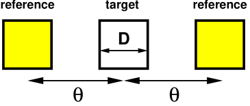
Figure 1: Measurement configuration to compute the structure noise. Gautier et al. Gautier_92 (1992) and Helou & Beichman Helou+Beichman_90 (1990) derived their results for the resolution limit $\rm\theta_{min}=2\,D$. In Sect. 3.3 we also consider the cases of $\rm\theta=k{\cdot}D,k=2...7$

Gautier et al. Gautier_92 (1992) pointed out that the Fourier power spectra of the IRAS 100$\mu$m scans were generally well represented by a power law, and that the structure noise can be linked to the parameters of the power spectra by the following relation:

$$\rm N\leavevmode\nobreak\ {\propto}\leavevmode\nobreak\ \Big{(}{d\over{d_{0}}}\Big{)}^{1-{{\alpha}\over{2}}}\times P_{0}^{1\over{2}}$$ (3)

where $\rm d^{-1}$ is the spatial frequency, $\rm d_{0}^{-1}$ is a reference spatial frequency, P₀ is the Fourier power at d${}^{-1}_{0}$, and $\alpha$ is the spectral index of the Fourier power spectrum. It was also found that most scans can be described by the empirical relationships $\alpha$ $\approx$ 3 and $\rm P_{0}\propto{\langle}B{\rangle}^{3}$.

Based on the IRAS results Helou & Beichman Helou+Beichman_90 (1990) (H&B) proposed a practical formula to predict the cirrus confusion noise, assuming that the empirical relationships of Gautier et al. Gautier_92 (1992) are valid at other wavelengths, too. They also took into account that at the resolution limit of the telescope $\rm d/d_{0}$ can be expressed by the resolution parameter of Fraunhofer diffraction, $\rm\lambda/D_{t}$, where $\lambda$ is the wavelength of the measurement and $\rm D_{t}$ is the diameter of the telescope primary mirror. Under these terms they expressed the cirrus confusion noise as:

$$\rm{{N_{H{\&}B}}\over{1\,mJy}}=0.3{\times}\Big{(}{{\lambda}\over{100\,{\mu}m}}\Big{)}^{2.5}\Big{(}{{D_{t}}\over{1\,m}}\Big{)}^{-2.5}\Big{(}{{\langle B_{\lambda}\rangle}\over{1\,MJysr^{-1}}}\Big{)}^{1.5}$$ (4)

Here $\rm B_{\lambda}$ is the surface brightness at the wavelength of the observation. The formula shows that the confusion noise depends on the wavelength in two separate ways: (1) via the variation of the surface brightness (spectral energy distribution of the emitting medium) and (2) via the dependence of the resolution parameter on $\lambda$. This relation which is valid for the standard measurement configuration as defined in Fig. 1 has been widely used for preparing far-infrared space telescope observations, and applied even for other configurations. The first noise analysis of four ISOPHOT maps was performed by Herbstmeier et al. Herbstmeier (1998), carrying out the first high spatial resolution study of the galactic cirrus at $\lambda{>}$100$\mu$m. They proved that the ISOPHOT sensitivity at far-infrared wavelengths is limited by sky confusion noise rather than by instrumental uncertainties.

The confusion noise caused by the CFIRB has different properties from the cirrus confusion noise. It can be represented by a Poissonian spatial distribution, therefore the confusion noise value is independent of the separation between the target and the reference positions. Ackermann et al. Ackermann92 (1992) investigated the sensitivity limits, including the effect of the CFIRB, for ISOPHOT and predicted that the long wavelength observations would be limited by galaxy confusion in the regions of faintest cirrus. Recently Lagache & Puget Lagache+Puget_2000 (2000), Matsuhara et al. Matsuhara (2000) and Juvela et al. (for an overview see Lemke et al. Lemke2000 (2000)) analysed ISOPHOT maps and separated the cirrus and extragalactic components. They announced the detection of the CFIRB with a fluctuation power in the range of $\rm 5-12{\times}10^{3}\,Jy^{2}sr^{-1}$ at 170 and 180 $\mu$m, close to the predictions of Guiderdoni et al. Guiderdoni_97 (1997). This leads to a galaxy confusion noise limit of 13–22 mJy for ISOPHOT at this wavelength.

For this paper we analysed 175 suitable far-infrared maps from the ISO Archive. Our goals were (1) to test the applicability of the Helou & Beichman Helou+Beichman_90 (1990) formula, especially at $\lambda\,>$ 100 $\mu$m; (2) to determine the relative contributions of the galactic cirrus and the extragalactic components in the faintest regions of the sky; (3) to derive an easy-to-use formalism for predicting the total sky confusion noise for instruments on ISO, SIRTF and HERSCHEL and for various measurement configurations, and (4) to determine the Cosmic Far-Infared Background Radiation via its fluctuations.

2 Observations and data analysis

2.1 Selection of ISOPHOT maps

We selected 175 maps from the ISO Archive (Kessler et al., Kessler2000 2000), observed in the 90 to 200 ${\mu}$m wavelength range, covering 40 different sky regions. All maps were obtained with the ISOPHOT instrument (Lemke et al., Lemke_96 1996) on-board the ISO satellite (Kessler et al., Kessler_96 1996), in the PHT22 raster observing mode (Laureijs et al., Laureijs2000 2000). Our selection criteria were that the maps should be larger than 5$\times$5 raster points, corresponding to $\sim$ 8^′ $\times$ 8^′ for the C100 (3$\times$3 pixel array, 46″ pixel size) and C200 (2$\times$2 pixel array, 92″ pixel size) detectors. Some maps were observed with full oversampling, i.e. the field was redundantly covered without gaps between detector pixels. The final map images are a composite of the individual array images on the different raster positions. The size of the image pixels is always a detector pixel.

We excluded maps with obvious individual structures (resolved stars, galaxies, planetary nebulae, etc.). The number of selected maps is 94, 4, 65 and 12 using the C1_90, C1_100, C2_170 and C2_200 filters, respectively, and they cover a wide range of surface brightnesses ($\sim$ 1–100 MJysr^-1). A more detailed description of the maps will be presented in a forthcoming paper (Kiss et al. 2001, in prep.) dealing with the spatial structure of the extended emission.

2.2 Data reduction

Basic data reduction was performed using the ISOPHOT Interactive Analysis software, PIA V8.2 (Gabriel et al., Gabriel97 1997) with the standard batch mode set-up. Flat-fielding had to be applied, which corrects for the residual responsivity differences of the individual detector pixels. We chose the First Quartile Normalization method, which uses the first quartiles of the maps’ brightness distribution, computed for each detector pixel, for normalization. The reliability of this statistical flat-field method was tested in the case of oversampled maps, were redundant observations of the same sky position by each detector pixel are available. These tests confirmed that the First Quartile Normalization gives accurate flat-field values, and was therefore adopted for this analysis.

The maps still contain the zodiacal light (ZL) emission, and a contribution from the CFRIB. The zodiacal emission does not contribute to the sky confusion noise, because its distribution is smooth on the scale of our maps (Ábrahám et al., Abraham97 1997). Therefore, we can eliminate it from the total brightness. First, we determined the non color corrected ratio of the ZL–to–total emission at the DIRBE wavelengths, using the COBE/DIRBE weekly maps and the COBE/DIRBE sky and zodi atlas (Hauser et al.Hauser98 (1998), Kelsall et al. Kelsall (1998)). We colour corrected the ZL component adopting a spectral energy distribution (SED) shape of a black body with a temperature of 270 K (Leinert et al. Leinert (2001) find 255 K $\leq$ T_ZL $\leq$ $297\,K$). The difference between the uncorrected total and ZL emission was color corrected by assigning a cirrus SED to it, assuming a 20 K modified black body with $\rm\nu^{2}$ emissivity law. Then interpolating the corrected ratios in between the COBE/DIRBE wavelengths, we estimated the ratios of the ZL-to-total emission for the ISOPHOT filter central wavelengths. The absolute ZL contribution in the ISOPHOT maps was computed by multiplying this ratio with the average total brightness measured by ISOPHOT (see also Héraudeau et al., Heraudeau 2001).

The remaining surface brightnesses include the CFIRB and the cirrus emission. In Sect. 3 we calculate the sky confusion noise and in Sect. 4.2 we separate the cirrus and Extragalactic Background fluctuations, and derive the value of the CFIRB.

2.3 Instrument noise

The determination of the instrument noise is crucial in order to get the real value of the sky confusion noise. In addition to the basic noise components (read-out noise, dark current variations, etc.), we also include in the instrument noise uncertainties related to the generation of the final maps (flat-field).

There are several ways to determine the instrument noise. The fundamental difference between them is the time scale over which the noise estimation was taken. We examined the following four methods:

• Ramp-noise: Each measurement is composed of many individual integrations on each raster position. A set of non-destructive read-outs builds up an integration ramp whose slope provides the signal of this integration (Lemke et al., Lemke_96 1996). From each measurement we created two maps using the even and odd integration ramps separately. The instrument noise was calculated from the difference between the ’even’ and ’odd’ maps. This noise estimate provides information on the detector stability on a time scale of seconds, the typical difference between adjacent ramps.

• PIA-noise: PIA provides a determination of the signal uncertainty of the individual raster positions, which can also be adopted as an estimate of N_inst. It reflects the error propagation of random error components in (1) the linear fitting of the integration ramps, and (2) the averaging of all signals per raster point . The time scale here is the time spent on an individual raster position, typically in the order of a minute.

• Flat-field-noise: This noise value was calculated from the variation of the brightness at the same sky position in maps created from individual detector pixels (i.e. in case of pixel redundancy), after correction by the appropriate flat-fielding factors. Since these factors are kept constant for the whole map, although the detector pixels show different time dependent transient curves, this instrument noise estimate includes the effects of the long term changes in the detector behaviour. Therefore the time scale is the observational time of the whole map, typically in the order of an hour. Since the transient behaviour depends on the illumination level, the flat-field-noise may also depend on the brightness of the map.

• Repetition-noise: If a sky region has been observed several times, then it is possible to derive a noise value from the comparison of the individual maps. The typical time scale here is the difference in the observation dates. It provides a measure of the measurement reproducibility.

The ramp- and PIA-noise could be calculated for each map, but the flat-field-noise could be evaluated only in maps with full oversampling (see Sect. 2.1) and the repetition-noise was only computed for one particular sky region (Marano 1 field) consisting of several submaps, each observed four times. A comparison of the different noise estimates showed that the ramp-noise provided the lowest N_inst values, typically a factor of 2 lower than the PIA-noise. The flat-field noise was higher than the PIA one, and the repetition noise was found to be nearly identical to the flat-field-noise. Since in the case of the structure noise calculation (Eq. 1) the target and reference positions were observed at times typically separated by several minutes, the correct instrument noise should lie between the PIA- and the flat-field-noise values. To be on the safe side, we chose the value of the flat-field-noise, although it may represent a somewhat conservative estimate, which might cause a slight underestimation in the final confusion noise values. Since this noise value is not available for each map, we took the uncertainties provided by PIA and scaled them according to the mean ratio of 1.35 and 1.65 of the flat-field- and PIA-noise values for the C100 and C200 detectors, respectively.

Figure 2: Instrument noise values measured on the ISOPHOT maps. In the case of oversampled maps the flat-field noise, otherwise the scaled up PIA-noise was adopted. The mean scaling factor between the PIA- and the flat-field noise values are 1.35 and 1.65 for the C_100 and C_200 detectors, respectively. (a) C100 detector: C1_90 and C1_100 filters (plus signs and diamonds, respectively), (b) C200 detector: C2_170 and C2_200 filters (black dots and crosses, respectively)

The typical instrument noise values we found (see Fig. 2) are somewhat higher than that of other authors, e.g. a factor of 2 compared to Lagache et al. Lagache+Puget_2000 (2000). This discrepancy can be traced back to the co-addition of four independent maps in their case, reducing the final noise values by this factor.

Following Herbstmeier et al. Herbstmeier (1998) we assumed that the sky brightness fluctuations and instrument noise contributions are statistically independent, therefore the measured structure noise can be expressed as:

$$\rm N_{meas}^{2}\leq N^{2}+2\cdot N_{inst}^{2}$$ (5)

where $\rm N_{meas}$ is the measured structure noise, $\rm N$ is the real structure noise and $\rm N_{inst}$ is the instrument noise. We used this formula for the subtraction of the instrument noise from the measured noise, by assuming equality between the two sides of the expression. In order to test this assumption we compared the confusion noise values of four C2_170 maps, where the same sky region was mapped repeatedly. The confusion noise must be the same and only the instrument noise values can differ in repeated observations. Assuming equality in Eq. 5 we obtained identical confusion noise values for all four measurements and for any separations.

3 Results

3.1 Confusion noise at the resolution limit

Figure 3: Confusion noise at the resolution limit $\rm\theta_{min}$ vs. surface brightness of the fields. (a) ISOPHOT C100 filters, C1_90 and C1_100. (b) ISOPHOT C200 filters, C2_170 and C2_200. The symbols are the same as in Fig. 2

Fig. 3 presents our results on the sky confusion noise (after removing the instrument noise using Eq. 5) measured with the four ISOPHOT filters C1_90, C1_100, C2_170 and C2_200. We used the convention $\theta$ = 2D, defined by Gautier et al. Gautier_92 (1992) (see Sect. 1). Following the H&B formula (Eq. 4) we fitted the data points for each filter separately, assuming a power-law relationship between the confusion noise and the average brightness of the field, but also allowing a constant factor:

$$\rm{{N(\theta_{min})}\over{1\,mJy}}=C_{0}+{C_{1}}{\times}\Big{(}{{\langle\rm B\rangle}\over{1\,MJysr^{-1}}}\Big{)}^{\eta}$$ (6)

The coefficients C₀, C₁ and $\eta$ are listed in Table 1. In the case of the C1_100 and C2_200 filters no appropriate determination of the C₀ offset was possible due to the lack of faint regions. Eq. 6 can be used to predict the confusion noise for the ISOPHOT filters studied here. Our confusion noise values measured at 170 $\mu$m are in agreement with a value of 45 mJy obtained by Dole et al. Dole2001 (2001) in the FIRBACK regions, taking into account that their value is a source flux confusion limit, which differs from ours by the footprint-fraction and is therefore a factor of 2 higher.

filter	C1_90	C1_100	C2_170	C2_200
$\rm C_{0}$	6.6$\pm$1.9	–	10.2$\pm$2.5	–
$\rm C_{1}$	0.7$\pm$0.3	0.6$\pm$0.1	3.0$\pm$0.3	4.4$\pm$0.2
$\rm\eta$	1.55$\pm$0.12	1.53$\pm$0.28	1.47$\pm$0.11	1.56$\pm$0.19
$\rm\theta_{min}$	92″	92″	184″	184″
$\Omega$ ($\rm 10^{-7}$sr)	0.6469	0.7030	2.6438	2.8120

Table 1: Results of the fits using the measured values of the sky confusion noise at the resolution limit $\rm N(\theta_{min})$ and the average surface brightness of the field $\langle B\rangle$ (see also Eq. 6 and the text for details). Separation limit and effective solid angle values are also presented. In the case of the C1_100 and C2_200 filters no appropriate determination of the C₀ offset was possible due to the lack of faint regions.

3.2 Comparison with the H&B formula

Figure 4: Confusion noise at the resolution limit determined by this study as compared to the prediction of Helou & Beichman Helou+Beichman_90 (1990). The symbols are the same as in Fig 2.

In Fig. 4 we compare our results with the predictions of the H&B formula (Eq. 4). In the surface brightness range where the cirrus emission dominates (5–30 MJysr^-1) the H&B formula predicts confusion noise values within a factor of 2 of our results. The scatter cannot be attributed to measurement uncertainties, and probably it reflects the physical differences among the fields. For the brightest fields the H&B formula seems to systematically overestimate the measured confusion noise values. Such regions, however, contain molecular clouds, therefore they may have different spatial structure from a cirrus region and should be described by a different power law. The figure also shows a large discrepancy at low surface brightness which could well be treated by the introduction of an offset (see above). A possible explanation of the deviations in the faint range is discussed in Sect. 4.2.

Figure 5: C₁ coefficients of the fits in Table 1 vs. the appropriate wavelength (logarithmic-logarithmic plot).

Although the H&B formula gives rather good predictions for the surface brightness range it was developed for (5–30 MJysr^-1), its coefficients, especially the three exponents, rely partly on the analysis of IRAS 100$\mu$m data, partly on theoretical considerations. Our data set offers a unique chance to test some of these exponents for the first time. The dependence of the confusion noise on the surface brightness was described by H&B using a power law with an exponent of 1.5 (Eq. 4), independently of the wavelength. This exponent $\eta$ was determined by our fits for four wavelengths in Sect. 3.1. The measured values in Table 1 are very close to the value of 1.5, proving the wavelength independence of this exponent.

In the next step we tested the dependence of the confusion noise on the resolution parameter $\rm\lambda/D_{t}$, also assumed to be in the form of a power law with an exponent of 2.5 by H&B (Eq. 4). Since the diameter of the telescope mirror $\rm D_{t}$ is the same regardless of the wavelength, in Fig. 5 we plotted the wavelength dependence of the C₁ coefficient from Table 1. The figure confirms the assumption of a power law, and gives an exponent of 2.53$\pm$0.31, in agreement with the value in Eq. 4. The dependence of the confusion noise on the diameter of the telescope (Eq. 4) was not possible to check, since the telescope mirror of ISO had the same size as that of IRAS. Our results verify exponents of the H&B formula for the first time by observations over a wide range.

3.3 Confusion noise for larger separations

The H&B formula provides information only on the measurement configuration presented in Fig. 1, at the resolution limit $\rm\theta_{min}$. However, in many applications the beam separation may be different. In most ISOPHOT measurements the observer was allowed to specify any separation up to 3′. Staring on-off measurements and sparse maps allowed even larger separations (Laureijs et al., Laureijs2000 2000). Properties of the sky confusion noise for these cases were not investigated so far.

As indicated in Sect. 1, the ratio of the confusion noise values measured at different separations is sensitive to the spatial distribution of the dominant component of the emission (galactic cirrus or distant galaxies). We found that the dependence of the sky confusion noise on the separation between target and reference sky positions can be described by a simple power law:

$$\rm N(q\cdot\theta_{min})=N(\theta_{min})\times q^{\gamma}$$ (7)

where q=1,1$1\over 2$…3$1\over 2$ and $\rm\gamma$ is constant for a specific map. We fitted $\rm\gamma$ for all maps. The results are presented in Fig. 6, which suggests that the $\gamma$ value is a filter-independent parameter of the field, depending only on the surface brightness.

Figure 6: $\gamma$ values of the $\rm N(q\cdot\theta_{min})=N(\theta_{min}){\cdot}q^{\gamma}$ fits for four ISOPHOT filters versus the surface brightness of the fields (see the text for details). The symbols are the same as in Fig. 2

For faint fields $\gamma$ is close to zero, while it increases strongly with increasing surface brightness. We found that the behaviour can be approximated by the following relation (dotted curve in Fig. 6):

$$\rm\gamma=\left\{\begin{array}[]{lr}0.02&\rm\,\,\,\,\,if\,\,\,{\langle\rm B\rangle}\leq\rm 3\,MJysr^{-1}\\ 0.65{\times}{\rm log_{\rm 10}}{\langle\rm B\rangle}-0.26&\rm\,\,\,\,\,if\,\,\,{\langle\rm B\rangle}>3\,MJysr^{-1}\end{array}\right.$$ (8)

Eq. 7 and 8 together with Eq. 6 and the coefficients in Table 1 provide a practical tool for the estimation of the confusion noise for a large variety of measurements.

4 Discussion

4.1 Variations of $\huge\gamma$

As shown in Sect. 3.3, for low surface brightness fields the $\gamma$ values are close to zero. In those regions the noise distribution differs from that expected for the galactic cirrus (see e.g. Ackermann et al., Ackermann92 1992)), originating from its multifractal structure. $\gamma\approx$ 0 is typical for a Poissonian distribution.

Higher $\gamma$ values in brighter regions may be caused by the cirrus structure. Despite this general trend the scatter of $\gamma$ at higher surface brightness is relatively large and there are a few regions measured by the C1_90 filter with high $\gamma$ values at low brightness. These discrepancies are probably caused by real physical differences between the fields. The $\gamma$ parameter depends on the spectral index of the Fourier power spectrum of the field (cf. Eq. 3). This relationship will be analysed in detail based on experimental data in a forthcoming paper (Kiss et al. 2001, in prep.). Differences in physical properties may originate in different chemical/dust composition, spatial structure, gas-to-dust or molecular-to-neutral gas ratio.

4.2 Fluctuations due to the Extragalactic Background

4.2.1 Findings from this work

When fitting the sky confusion noise as a function of the surface brightness in Sect. 3.1 a constant term C₀ was allowed for. At both 90 and 170 $\mu$m definite positive values were obtained at the 3–4$\sigma$ significance level. Assuming that the cirrus confusion noise follows the power law behaviour also at very low surface brightness, this offset cannot be attributed to cirrus. The spatial distribution of the confusion noise below $\sim$3 MJysr^-1 has different characteristics than in brighter cirrus fields (see Sect. 3.3 and Fig. 6). The likely origin of this noise component, as suggested by its invariability with the surface brightness and its Poissonian spatial distribution, would be the fluctuation due to the Cosmic Far-Infrared Background (CFIRB).

If this interpretation is correct, than Eq. 6 provides a new method to determine the value of the CFIRB fluctuation. The features of this method are (1) the subtraction of the cirrus component via its dependence on the surface brightness and (2) that this dependence is calibrated simultaneously on the brighter cirrus fields of the same database. An advantage of this method is the utilization of the largest ISOPHOT database for the determination of the CFIRB fluctuations. The results are not sensitive to characteristics in individual fields. On the other hand, any uncertainty in the surface brightness calibration of the cirrus would introduce an uncertainty in the fluctuation value, too.

The values given by the fitting procedure in Sect. 3.1 for the C₀ coefficients are 6.6$\pm$1.9 and 10.2$\pm$2.5 mJy at 90 and 170 $\mu$m, respectively. In this fitting the surface brightness values still included a contribution from the CFIRB itself. Subtraction of the CFIRB increases the fluctuation amplitudes. Varying the CFIRB surface brightness B₀ within the assumed range of 0.1 to 1.5 MJysr^-1 and subtracting it from the total surface brightness we used Eq. 6 to derive the corresponding C₀ coefficients which were then transferred to surface brightness fluctuations $\delta$B₀ as $\delta$B₀ = C₀/$\Omega_{\lambda}$, where $\Omega_{\lambda}$ is the effective solid angle of a detector pixel (see Table 1).

The results are shown in Fig. 7. As it can be seen in this figure, the dependence of $\delta$B₀ on the assumed value of B₀ is not very strong, therefore, regardless of the real value of the CFIRB, a well confined value of $\delta$B₀ can be derived. We obtained C₀ = 7$\pm$2 mJy ($\delta$B₀ = 0.11$\pm$0.03 MJysr^-1) at 90$\mu$m and C₀ = 15$\pm$4 mJy ($\delta$B₀ =0.06 $\pm$0.02 MJysr^-1) at 170$\mu$m.

In most models CFIRB fluctuations are caused by galaxy clustering, and, due to the flat power spectrum, the $\delta$B₀/B₀ value is constant in the 1°  to 5′  resolution range (Kashlinsky et al. Kashlinsky (1996), Haiman & Knox Haiman (2000)). At finer resolution (higher spatial frequencies) effects by individual galaxies have to be considered. An estimate of $\delta$B₀/B₀ (or $\delta$($\nu$I_ν)/($\nu$I_ν)) can be performed following Bond et al. Bond (1986), assuming biased galaxy clustering. Using eq. 6.35 from Bond et al. Bond (1986), the fluctuation ratio is : $\rm\delta(\nu I_{\nu})/(\nu I_{\nu})=0.05\times(1\arcmin/\sigma)^{0.4}$ where $\sigma$ is the smoothing angle, and the beam profile is approximated by a Gaussian. Equations 6.24 and 7.2 in Bond et al. Bond (1986) give $\sigma$ = 12″  and 23″  for 90 and 170 $\mu$m, respectively, for ISOPHOT. From this results $\delta$($\nu$I_ν)/($\nu$I_ν) = 10% at 90 $\mu$m and $\delta$($\nu$I_ν)/($\nu$I_ν) = 7% at 170 $\mu$m.

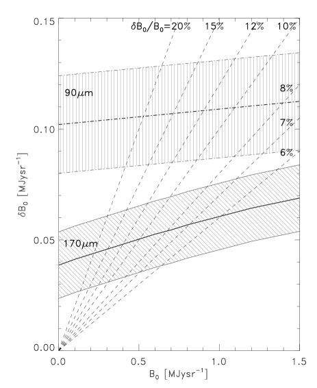
Figure 7: CFIRB fluctuation amplitudes versus the CFIRB absolute level assumed. The hatched regions represent the formal errors of the fits in Eq. 6 for 90 and 170 $\mu$m. A set of dashed lines marks $\delta$B₀/B₀ = 6, 7, 8, 10, 12, 15 and 20%.

At 170 $\mu$m $\delta$B₀/B₀ = 7% provides B₀ = 0.8$\pm$0.2 MJysr^-1 equivalent to $\nu$I_ν = 14$\pm$3 nWm^-2sr^-1.

At 90 $\mu$m the dependence of $\delta$B₀ on B₀ is even weaker than at 170 $\mu$m, therefore a well defined value of 0.11$\pm$0.03 MJysr^-1 can be determined. The B₀ value of 1.1$\pm$0.3 MJysr^-1, equivalent to $\nu$I_ν = 37$\pm$10 nWm^-2sr^-1), is the same as the average surface brightness of the faintest 90 $\mu$m maps in our data set. The expected cirrus contribution in these fields – predicted from the $\sim$0.8 MJysr^-1 value at 170 $\mu$m by using a typical cirrus spectrum (modified black-body SED, $\rm\nu^{2}$ emissivity law, 20 K temperature) – is about 0.3 MJysr^-1. This result suggests that the 1.1 MJysr^-1 is an upper limit and the most likely value of the CFIRB lies at the lower end of the uncertainty range, i.e. $\sim$0.8 MJysr^-1 equivalent to $\nu$I_ν = 30 nWm^-2sr^-1.

Our results satisfy the three main criteria of a CFIRB detection as proposed by Hauser & Dwek Hauser+Dwek (2001): (1) We achieved a detection of a positive value of the fluctuation amplitudes (and therefore the absolute value as well) at 90 and 170 $\mu$m at the 4$\sigma$ level. (2) We removed the contribution by all known foreground (noise) emitters (zodiacal light, instrument noise, galactic cirrus). The properties of the spatial distribution related to the remaining noise term agree with that expected for the CFIRB fluctuations. (3) Due to the statistical nature of our method, the detection of the same well defined positive constant term in different areas of the far-infrared sky indicates the isotropy of this component.

4.2.2 Comparison with other results

The 170 $\mu$m confusion noise C₀ = 15$\pm$4 mJy is in good agreement with the 13 mJy obtained by Juvela et al. (see the overview of Lemke et al. Lemke2000 (2000)), and somewhat lower than the values of 18 mJy determined by Lagache & Puget Lagache+Puget_2000 (2000) from the analysis of the Marano 1 field and the 22 mJy derived by Matsuhara et al. Matsuhara (2000) from the investigation of the Lockman Hole region. Our derived CFIRB value of 14$\pm$3 nWm^-2sr^-1  is the same as predicted from models by Pei et al. Pei (1999). Also the COBE measurements calibrated on the FIRAS photometric scale (Hauser et al. Hauser98 1998,  for an overview see Hauser & Dwek 2001) give quite similar levels (15$\pm$6 nWm^-2sr^-1  at 140$\mu$m and 13$\pm$2 nWm^-2sr^-1  at 240$\mu$m) despite the big difference in spatial resolution.

The 90 $\mu$m confusion noise C₀ = 7$\pm$2 mJy is close (although somewhat lower) to the 11 mJy found by Matsuhara et al. Matsuhara (2000). With regard to the 90 $\mu$m absolute value Schlegel et al. Schlegel98 (1998) provided the same 1.1 MJysr^-1 value as an upper limit for the CFIRB at 100 $\mu$m, and also Lagache et al. Lagache2000 (2000) and Finkbeiner et al. Finkbeiner (2000) reported a detection of a 100 $\mu$m CFIRB level of 23$\pm$6 nWm^-2sr^-1  and 25$\pm$8 nWm^-2sr^-1 , respectively, which are close to our upper limit.

4.3 Confusion limits for far-infrared space telescopes

After the comparison of instrument and confusion noise values (see Fig. 2 and 3) it is obvious that even in the faintest sky regions the instrument noise is below the sky confusion noise by a factor of 2–3 for the C2_170 filter. This confirms the results of Herbstmeier et al. Herbstmeier (1998), showing that the ISOPHOT C200 detector was limited by sky brightness fluctuations rather than by instrumental effects. In the case of the C1_90 filter the instrumental and confusion noise are similar in strength at the resolution limit. Since our results confirm the applicability of the H&B formula, the predictions made for other space missions with telescopes of a similar size (SIRTF, Astro-F) on the basis of this formula can be trusted. Predictions made for the HERSCHEL satellite (3.6m mirror), however, still have to partially rely on assumptions, since we were not able to test the dependence of the confusion noise on the diameter of the telescope primary mirror. It remains to be demonstrated that the spatial structure of cirrus does not change below the resolution limit of ISO.

5 Summary

Using measurements obtained with ISOPHOT we investigated the properties of the sky confusion noise on a large sample of maps in the 90 $\leq$ $\lambda$ $\leq$ 200 $\mu$m wavelength range. We described the dependence of the sky confusion noise on the surface brightness for four selected ISOPHOT filters. We verified that the confusion noise scales as N $\propto\langle\rm B\rangle^{1.5}$ for the resolution limit, independent of the wavelength. We also confirmed that, due to the dependence on the resolution parameter, N $\propto\lambda^{2.5}$ at $\rm\lambda\geq 100$ $\mu$m. According to our results for cirrus fields with $\rm\langle\rm B\rangle>5$ MJysr^-1 the Helou & Beichman Helou+Beichman_90 (1990) formula predicts confusion noise values within a factor of 2. The scaling of the noise value at different separations between target and reference positions was investigated for the first time, providing a useful formula to estimate the confusion for different separations, too. At 90 and 170 $\mu$m a noise term with a Poissonian spatial distribution was detected in the faintest fields ($\rm\langle B\rangle\leq 3-5\,MJysr^{-1}$), which we interpret as fluctuations in the Cosmic Far-Infared Background (CFIRB). With a ratio of the fluctuation amplitude to the absolute level of 10% and 7% at 90 and 170 $\mu$m, respecively, we determined the fluctuation amplitudes and the surface brightness of the CFIRB. The fluctuation amplitudes are 7$\pm$2 mJy and 15$\pm$4 mJy at 90 and 170 $\mu$m, respectively. We obtained a CFIRB surface brightness of B₀ = 0.8$\pm$0.2 MJysr^-1 ($\nu$I_ν = 14$\pm$3 nWm^-2sr^-1) at 170 $\mu$m and an upper limit of 1.1 MJysr^-1 ($\nu$I_ν = 37 nWm^-2sr^-1) at 90$\mu$m.

- (1) Ábrahám P., Leinert Ch., Lemke D., 1997, A&A 328, 702
- (2) Ackermann E., Hajduk C., Lemke D., 1992, Sensitivity Limits for the Photopolarimeter ISOPHOT, In: Infrared Astronomy with ISO, (eds.) Th. Encrenaz and M.F. Kessler, Nova Science Publisher, p.79.
- (3) Bond J.R., Carr B.J., Hogan C.J., 1986, ApJ 428, 306
- (4) Dole H., Gispert R., Lagache G., et al., 2001, A&A 372, 364
- (5) Finkbeiner D.P., Davis M., Schlegel D.J., 2000, ApJ 544, 81
- (6) Gabriel C., Acosta-Pulido J., Heinrichsen I., et al., 1997, The ISOPHOT Interactive Analysis PIA, a Calibration and Scientific Analysis Tool, In: ADASS VI, ASP Conference series vol. 125, (eds.) Hunt G., Payne H.E., p. 108
- (7) Gautier III T.N., Boulanger F., Pérault M., Puget J.L., 1992, AJ 103, 1313
- (8) Guiderdoni B., Bouchet F.R., Puget J.L., Lagache G., Hivon E., 1997, Nature 390, 257
- (9) Haiman Z., Knox L., 2000, ApJ 530, 124
- (10) Hauser M.G., Arendt R.G., Kessel T., et al., 1998, ApJ 508, 25
- (11) Hauser M.G., Dwek E., ASTRO-PH 0105539, to appear in Annu. Rev. Astron. Astrophys.
- (12) Helou G., Beichman C.A., 1990, The confusion limits to the sensitivity of submilimeter telescopes, In: From Ground-Based to Space-Borne Sub-mm Astronomy, Proc. of the 29th Liège International Astrophysical Coll., ESA Publ., p. 117. (H&B)
- (13) Héraudeau Ph., Ábrahám P., Klaas U., Kiss Cs., del Burgo C., ”Systematic comparison of ISOPHOT and DIRBE Surface Brightness Calibration”, In: ‘The calibration legacy of the ISO Mission’, (eds.) Metcalfe L. et al., ESA Special Publications Series, Vol. 481., in press
- (14) Herbstmeier U., Ábrahám P., Lemke D., et al., 1998, A&A 332, 739
- (15) Kashlinsky A., Mather J.C., Odenwald S., 1996, ApJ 473, L9
- (16) Kelsall T., Weiland J.L., Franz B.A., et al., 1998, ApJ 508, 44
- (17) Kessler M.F., Steinz J.A., Anderegg M.F., et al., 1996, A&A 315, 27
- (18) Kessler M.F., Müller T.G., Arviset C., García–Lario P., Prusti T., 2000, The ISO Handbook Vol. I., ISO – Mission Overview, SAI-2000-035/Dc, Version 1.0, ISO Data Centre, Villafranca del Castillo
- (19) Lagache G., Abergel A., Boulanger F., Désert F.X., Puget J.-L., 1999, A&A 344, 322
- (20) Lagache G., Puget J.-L., 2000, A&A 355, 17
- (21) Lagache G., Haffner L.M., Reynolds R.J., Tufte S.L., 2000, A&A 354, 247
- (22) Laureijs R.J., Klaas U., Richards P.J., Schulz B. and Ábrahám P., 2000, The ISO Handbook Vol. V., PHT - The Imaging Photo-Polarimeter, SAI/99-069/Dc, Version 1.2, ISO Data Centre, Villafranca del Castillo
- (23) Leinert Ch., Ábrahám P., Acosta-Pulido J., Lemke D., Siebenmorgen R., 2001, A&A, submitted
- (24) Lemke D., Klaas U., Abolins J., et al., 1996, A&A 315, 64
- (25) Lemke D., Ábrahám P., Haas M., et al., 2000, ISOPHOT Surveys and the Extragalactic Background, In: The Extragalactic Background and its Cosmological Implications, IAU Symposium Vol. 204, (eds.) Harwit M., Hauser M.G., in press
- (26) Low F., Beintema D.A., Gautier T.N., et al., 1984, ApJ 278, 19
- (27) Matsuhara H., Kawara K., Sato Y., et al., 2000, A&A 361, 407
- (28) Pei Y.C., Fall M.S., Hauser M.G., 1999, ApJ 522, 604
- (29) Schlegel D.J., Finkbeiner D.P., Davis M., 1998, ApJ 500, 525