Topology and Polarisation of Subbeams Associated With
Pulsar B0943+10’s ‘Drifting’-Subpulse Emission:
II. Analysis of Gauribidanur 35-MHz Observations

Abstract

In the previous paper of this series Deshpande & Rankin (2001) reported results regarding subpulse-drift phenomenon in pulsar B0943+10 at 430 MHz and 111 MHz. This study has led to the identification of a stable system of subbeams circulating around the magnetic axis of this star. Here, we present a single-pulse analysis of our observations of this pulsar at 35 MHz. The fluctuation properties seen at this low frequency, as well as our independent estimates of the number of subbeams required and their circulation time, agree remarkably well with the reported behavior at higher frequencies. We use the ‘cartographic’-transform mapping technique developed in Paper-I to study the emission pattern in the polar region of this pulsar. The significance of our results in the context of radio emission mechanisms is also discussed.

1 Introduction

The foregoing paper by Deshpande & Rankin (2000; hereafter Paper-I) reported detailed studies of the steady subpulse drift of pulsar B0943+10, using Arecibo polarimetric observations at 430 and 111 MHz. They introduced several new techniques of fluctuation-spectral analysis and addressed the possible aliasing of the various features in an effort to determine their true frequencies. The paper further introduced a ‘cartographic’ transformation (and its inverse) which relates the observed pulse sequence to a rotating pattern of emission above the pulsar polar cap. This approach provided a direct means of determining some of the key parameters characterizing this underlying source pattern and its stability—thus facilitating a fuller comparison with the predictions of pulsar emission theories (see also Deshpande & Rankin, 1999, hereafter DRa).

While the Arecibo observations in Paper-I document a great deal about 0943+10’s remarkable ‘drift’ behavior, they also demonstrate the need for further studies of different types and at various wavelengths. The 430-MHz observations, for instance, sample only the outer radial periphery of the subbeams defining the overall hollow emission cone of the pulsar—and this is apparently a major reason for its unusually steep spectrum above 100 MHz. Observations at decameter wavelengths are particularly interesting, both because the pulsar is expected to be relatively brighter and also because they provide a means of exploring the character of the larger low frequency conal beam size [often attributed to ‘radius-to-frequency mapping’ or ‘RFM’; e.g. see Cordes, 1978, and the generally assumed dipolar field geometry]. At 35 MHz, then, we would expect our sightline to sample the region of emission more centrally, with the result that, the full radial extent of the subbeams would be ‘seen’ and the high frequency ‘single’ profile would be well-resolved into a ‘double’ form. The character of the low frequency emission pattern would also be of interest—both in its own right and as compared to those at higher frequencies—for what insights it might provide into the manner in which emission sites at different heights/frequencies are connected.

Below, we report the results of our analysis of pulse-sequence observations of B0943+10 at 35 MHz. Our observations and analysis procedures are outlined in the next section. Subsequent sections then describe the results of fluctuation-spectral analysis, the implied subbeam-system topology, and the derived polar emission maps [some preliminary results were reported earlier in Asgekar & Deshpande (2000)].

2 Observations and Analysis

Observations of this pulsar were carried out as a part of a new programme of pulsar observations (Asgekar & Deshpande, 1999) initiated at the Gauribidanur Radio Observatory (Deshpande, Shevgaonkar & Shastry, 1989) with a new data acquisition system (Deshpande, Ramkumar & Chandrasekaran, 2000). The pulsar was observed for a typical duration of $\ga{1000}$ s in each session. Several such observations were made during the spring of 1999. We discuss two data sets below, denoted as ‘C’ and ‘G’, which were observed on February 7 and 13, respectively.

From the signal voltages (over a 1-MHz bandwidth) sampled at the Nyquist rate with 2-bit, 4-level quantization, a time-series matrix of intensity with a desired spectral and temporal resolution (equivalent to data from a spectrometer) was obtained. After checking for, and excising, interference in the spectral as well as the time domains, the different spectral channel data were combined after appropriate dispersion-delay correction. The resulting time sequence was resampled at the desired intervals of the rotation phase of the pulsar to obtain a gated pulse sequence for a specified gate-width (typically $\sim 100^{\circ}$).

Our techniques of spectral analysis for the 35-MHz observations are virtually identical to those used in Paper-I, so we will rely on its fuller descriptions of these methods and request that the reader refer to them there.

Fluctuation Spectra and Aliasing

Our 35-MHz observations lack the sensitivity to detect a majority of the individual pulses in a sequence, let alone to identify their drift pattern. Any such drift can best be investigated using longitude-resolved fluctuation (hereafter, ‘LRF’) spectra (Backer, 1973). Figure 1 then gives such a spectrum for the G sequence. Note in particular the prominent peaks at 0.459 c/$P_{1}$ (feature 1) and 0.027 c/$P_{1}$ (feature 2). Feature 1 is associated with the observed subpulse drift at meter wavelengths; it is barely resolved here, implying a Q of $\geq$500. This clearly indicates that the underlying modulation process is also quite steady at decameter wavelengths. The modulation frequency is slightly different for the C observation, but small variations ($\leq 0.5\%$) were also noted by Deshpande & Rankin (Paper-I), so are not surprising. The important questions we wish to address are the effect of a possible aliasing of feature 1 and its relation to feature 2.

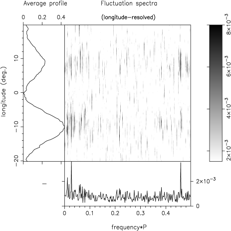
Figure 1: LRF spectrum of the 34.5-MHz G sequence, using 512 pulses. The body of the figure gives the amplitude of the features in (arbitrary) grey-scale displayed on the right. The average profile of the pulsar is shown in the left-hand panel, and the integral spectrum is given at the bottom of the figure (see Paper-I:Figure 1 for details).

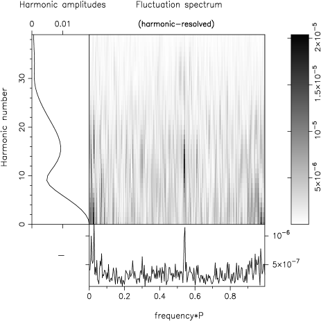
Figure 2: HRF spectrum of the 34.5-MHz G sequence. The amplitude of the frequency components at the fundamental rotation frequency (1/P₁) and its harmonics are plotted in the left-hand panel of the diagram. The body of the figure gives the amplitude of the other frequency components in the spectrum upto 40/P₁ in (arbitrary) grey-scale, displayed on the right.The bottom panel shows the sum of the frequency components, collapsed onto a 1/P₁ interval. See Paper-I: Figure 4 for details.

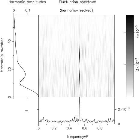
Figure 3: HRF spectrum of the 34.5-MHz C sequence using 128 pulses. The feature 2 (seen in G sequence) is not detectable here.

To assess the issue of aliasing, we compute a harmonic-resolved fluctuation spectrum (hereafter, ‘HRF’ spectrum; see Paper-I: Figure 4) by Fourier transforming the continuous time series. Such a time series is reconstructed from the (gated) pulse sequence by setting the intensity in the off-pulse region to zero. A spectrum constructed in this manner for the G observation is displayed in Figure 2. Note that amplitude modulation would produce a pair of features in the HRF spectrum, symmetric about frequency 0.5 c/$P_{1}$ and with nearly equal amplitudes; whereas, phase modulation would produce a strong asymmetry in the pair amplitudes, as exemplified in Figure 2. We can then see that the fluctuation feature at 0.541 c/$P_{1}$ is associated with a phase modulation, and further appears as the first-order aliased feature 1 at 0.459 c/$P_{1}$ in the LRF spectrum of Figure 1. A similar conclusion regarding the nature of the modulation can be drawn by looking at the rate of change of the modulation phase with longitude (see Figure 5), which is $26^{\circ}/^{\circ}$—too large for a mere amplitude modulation.

We now fold the pulse sequence at the modulation period $P_{3}$ in Figure 4. The drift-bands related to the two components are clearly visible and exhibit a phase difference between the modulation peaks. The ‘bridge’ region between the two average-profile components exhibits little discernible fluctuation power, so we could be missing one or more drift bands in this longitude interval. We therefore express the modulation phase difference between the two components as, $\Delta{\theta}=2\pi\,(0.8+m)$ (where, m = 0,1,2..). If the modulation under the two components is caused by ‘passage’ of the same emission entity through our sightline as it rotates around the magnetic axis, the average profile-component separation in longitude of about 20^∘ suggests a $P_{2}$ value of about $11^{\circ}$ for $m=1$—which is consistent with the estimates at meter wavelengths. Further, the azimuth angle subtended by the profile components at the magnetic axis can be computed using our knowledge of the viewing geometry [referring to eq. (3) of Paper-I], and is estimated to be about $33^{\circ}$. We adopt here the values of $\alpha$ and $\beta$, determined in Paper-I—that is, 11.64^∘ and -4.31^∘, respectively. It follows that the magnetic azimuthal separation between the subbeams would be about $18^{\circ}$ (corresponding to $P_{2}$), suggesting a rotating system of about 20 subbeams.

It is clear that the 35-MHz observations exhibit phase modulation very similar to that noted at higher frequencies, and the true modulation frequency is near 0.541 c/$P_{1}$, implying that $P_{3}=1.848{P_{1}}$. This means that the subpulse drift proceeds in the direction opposite as that of star’s rotation. Some enhancement in the spectral power is evident at 0.06 c/P₁, corresponding to the aliased second harmonic of the primary modulation feature. The frequency and Q-value of the fluctuation features are in excellent agreement with those based on analysis of 430-MHz observations.

The feature 2, at about 0.027 c/P₁, is new and also has a high Q. As both LRF- and HRF-spectra show the feature at the same frequency, we conclude that it is not aliased and that 0.027 c/P₁ is its true frequency. It is important to note that this feature, seen in set G, is not apparent in the corresponding spectra of 111 and 430-MHz data (Paper-I), as well as in our other data sets at 35 MHz. We discuss its significance below.

The Amplitude-Modulation Feature, Subpulse Spacing and the Number of Rotating Subbeams

With an understanding of the intrinsic frequencies of the two principal features in the LRF spectrum, we can now explore a possible relationship between them. A straightforward calculation, $0.541/0.027={20}$, shows that the two features are harmonically related within their errors. We have looked for the sidebands (at $\pm$ 0.027 c/P₁) around the phase modulation feature at 0.541 c/$P_{1}$. Such side-bands were identified in some sections of the 430-MHz sequences (see Paper-I and DRa), but they occur in our data only at a much lower level of significance (e.g., see the central panel of Figure 1). The 0.027 c/$P_{1}$ feature, just as did the 430-MHz sidebands, suggests a slower amplitude modulation, with a periodicity, $\hat{P}_{3}$, of 37.5 $P_{1}$ or just 20 $P_{3}$. The magnetic azimuth angle corresponding to the longitude interval $P_{2}$ would be $\sim 18^{\circ}$, if a total of 20 subbeams were to be distributed more-or-less evenly around the magnetic axis, a value which is in excellent agreement with our estimate above, implying consistency with the viewing geometry as determined in Paper-I.

All these circumstances, along with the high $Q$s of the modulation features and their harmonic relationship, imply a stable underlying pattern of 20 subbeams, with the period of the low frequency feature (feature 2) providing a direct estimate of the circulation time of this pattern. This slow modulation may also be partially a phase modulation, considering the asymmetry in the features at 0.027 c/$P_{1}$ and 0.973 c/$P_{1}$ (see Figure 2). This would imply some non-uniformity in the spacing of the subbeams.

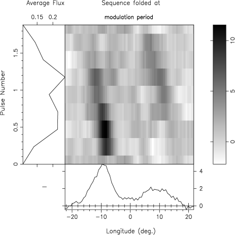
Figure 4: Diagrams showing the results of folding the C observation at the primary modulation period $P_{3}$. Note the separate ‘drift’ bands for two components in the central panel. The average profile is plotted in the bottom panel, and the average flux at a particular phase of modulation in the left-hand panel. Note that the ‘drift’ band for the trailing component peaks earlier than that for the leading component.

Figure 5: The phase of the primary modulation $P_{3}$ as a function of pulse longitude for the C observation, along with the average (solid curve) and modulated-intensity (dashed curve) profiles.

Figures 6 and 7 show the average polar emission patterns corresponding to the G and C observations, respectively. These patterns were reconstructed using the ‘cartographic transformation’ technique developed in Paper-I as well as the various parameters describing our viewing geometry of the pulsar determined there, but take all values of the circulation time ($\hat{P}_{3}$) from the present analysis. In assembling these maps, we make no use of the subbeam number once the circulation time has been determined directly; rather, the ‘cartographic transformation’ transforms the pulse sequence into the frame of the pulsar polar cap [see Paper-I : eqs. 5-8], so that the elements of the emitting pattern and their distribution can be viewed directly. In addition, the inverse ‘cartographic’ transform provides a useful means of assessing the consistency and uniqueness of the input parameters (see Deshpande, 1999 for details). In spite of our overall poor signal-to-noise observations, these ‘closure’ consistency checks show a remarkable sensitivity to the circulation time, the sign of $\beta$, and to the drift direction. Relative insensitivity to the other parameters, however, does not allow us to assess the viewing geometry independently.

Polar Emission Patterns at 35 MHz

Figure 6 shows the average emission pattern mapped using 512 pulses from the G sequence. Remarkably, the ‘active’ subbeams seem to occupy only about half of the conal periphery. Such a deep and systematic modulation in the subbeam intensity around the emission cone is completely consistent with the appearance of the slow modulation feature in the fluctuation spectra (see Figures 1 and 2). The emission pattern of the C observation in Figure 7, on the other hand, exhibits most of the 20 subbeams and a more-or-less uniform spacing—that is, an unsystematic pattern of intensities—a picture which is also entirely compatible with the observed absence of any significant slow modulation feature in its fluctuation spectra (Figure 3). It is worth mentioning that the power associated with the primary modulation (i.e. drift) is significantly higher in the C sequence than in the G observations.

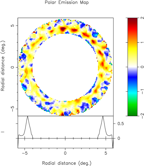
Figure 6: Average polar emission map made with 512 pulses from the G observation. Note the strong asymmetry about the magnetic axis. See text for details.

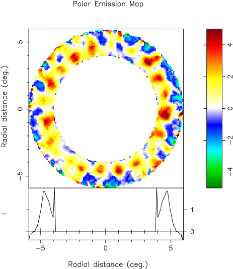
Figure 7: Average polar emission map made with 140 pulses from the C observation. Here we see a nearly full complement of subbeams, distributed evenly about the magnetic axis. See text for details.

It is clear from both the images that the sampling of the subbeams in the radial direction is more or less complete. This is significantly so in contrast with the partial sampling of the subbeams at 430 MHz. The situation is easily understood in terms of the larger angular radius of the radiation cone at low radio frequencies, which permits our fixed sightline to sample it more centrally. The slight elongation (in the azimuthal direction) apparent in the subbeam shape may not be real, perhaps resulting simply from slight jitter in the positions of the subbeams relative to the average.

A series of polar maps, each from successive subsequences (of duration $\geq\hat{P}_{3}$), were generated and viewed in a movie-like fashion Although individual frames have a reduced signal-to-noise ratio, certain significant characteristics can nonetheless be readily discerned. While some features are stable over only a few circulation times, most (e.g., the bright subbeams of the G sequence in Figure 6) remain relatively prominent over many hundreds of pulse periods. In both observations, in a set of successive frames of a movie, a few subbeams usually dominate others in intensity. Overall, the brightness of the subbeams was observed to fluctuate by up to about a factor of 4 over the length of the sequence.

In the G sequence a few subbeams are persistently bright, accounting for most of the power in the average profile. A very different behavior is seen in the C observation, where the subbeams are all very weak and unstable in the initial part of the sequence. Then, they gradually increase in intensity until most of the 20 subbeams constitute a more-or-less stable configuration—that depicted in Figure 7—for some four or five circulation times, whereupon they again gradually fade back into a disorganized pattern. The phase modulation feature is not readily detectable in either the pre- or post-bright phases. Neither, interestingly, are associated changes observed in the shape of the average profile; rather, it maintains a clear ‘B’-mode profile form, apart from the changes in the average intensity.

3 Discussion

In the foregoing paragraphs, we have outlined our analysis of the fluctuation properties apparent in the decametric emission of pulsar B0943+10, as well as our efforts to understand the underlying emission pattern responsible for them.

Although the signal-to-noise ratio of our 35-MHz observations is insufficient to detect most individual subpulses, we have demonstrated that the average fluctuation behavior can nonetheless be reliably characterized, because both the magnitude of the fluctuations is large and their pattern relatively stable. Indeed, such long sequences of pulses present an advantage (and opportunity) only if the underlying modulation is relatively stable over the relevant time scales, as in the present case. The primary phase-modulation frequency is observed to vary, but only on scales of many hundreds of pulse periods. Although the observed variations in the apparent $P_{3}$ might suggest corresponding fractional changes in the circulation time, they are more likely to be a manifestation of tiny (an order of magnitude smaller) fractional changes in the subbeam spacing.

Pulsar B0943+10 is unusual in that conal narrowing at frequencies above about 300 MHz causes its beam to progressively miss our sightline. For a given $\beta$, we expect our sightline to sample the radiation cone at different $\beta/\rho$ values, such that more central traverses occur at lower frequencies—the ‘single’ profile form of the pulsar at 430 MHz thus evolving smoothly into a well defined ‘double’ form as $\beta/\rho$ decreases sufficiently at longer wavelengths. The average profile of PSR 0943+10 at 35 MHz exemplifies this situation with an estimated $\beta/\rho$ of 0.78 (see Table II of Paper-I), corresponding to a nearly complete sampling of the radial ‘thickness’ ($\Delta\rho$) of the hollow-conical emission pattern. The fractional thickness of this conal beam $\Delta\rho/\rho$ is estimated to be about $15\%$, consistent with that estimated by Mitra & Deshpande (1999).

The average profile at decameter wavelength also shows asymmetry (the peak intensities of the two components around the apparent central longitude differ by a factor of about 2), so also the profile of modulated power (see Figure 5). Such an asymmetry, though striking, may be traceable to relatively small departures of the polar cap boundary from circularity, if the departures are comparable to the fractional thickness of the emission cone ($\Delta\rho/\rho$). A study, by Arendt & Eilek (2000), of the detailed shape of the polar-cap boundary and its dependence on the inclination angle $\alpha$, shows that an about 5% departure from circularity is expected for $\alpha=15^{\circ}$. Our results, together with those of Paper-I, should allow us to estimate the fractional non-circularity which would cause the observed asymmetries, and our efforts in this regard will be reported elsewhere.

The main results of our decametric study of PSR 0943+10’s fluctuation properties are as follows:

• We have shown that fluctuation spectra at decameter wavelengths also display a narrow feature with a high $Q$, which is related to the ‘drifting’ character of its subpulses.

• We have independently resolved how this feature is aliased and have determined the true frequency of the primary phase modulation.

• The high and low frequency features in the G sequence were found to be related harmonically (the former just 20 times the latter). Furthermore, weak sidebands appear to be associated with the primary phase-modulation feature, again suggesting that a slower fluctuation, of period $\hat{P}_{3}=20P_{3}$, is modulating the primary phase fluctuation.

• Since the viewing geometry at 35 MHz is too central ($\beta/\rho=0.78$) to follow the ‘drift’ band continuously across the pulse window, we have adopted different means of estimating the value of $P_{2}$, which at $11^{\circ}$ agrees well with that determined in Paper-I.

• Our observations lead to the conclusion that a system of 20 subbeams, rotating around the magnetic axis of the star with a circulation time $\hat{P}_{3}$ of about 37 $P_{1}$, is responsible for the observed stable subpulse-modulation behavior.

• Compared with the higher frequency maps, the 35-MHz maps sample the subbeams much more completely. However, the 35-MHz subbeams, on the whole, show much less uniformity in their positions and intensities.

• At both 35 MHz and the higher frequencies, the intensities of individual subbeams fluctuate, maintaining a stable brightness only for a few circulation times. The stability time-scales of the entire pattern appear roughly comparable between 35 MHz and 430 MHz.

Since the particle plasma responsible for the pulsar emission originates close to ‘acceleration’ zone (which is considered to be located near the magnetic polar cap), whereas the conversion to radio emission occurs at a height of several hundred kilometers above the stellar surface, we are led to conclude that the polar cap is connected to the region of emission via a set of ‘emission columns’. This picture is further supported by the very similar emission patterns observed at 35 MHz and 430 MHz—emitted, presumably, at significantly different altitudes in the star’s magnetosphere. If indeed some ‘seed’ activity results in the common character of the emission patterns at different frequencies, then the parameters describing the fluctuations (e.g. $P_{2},P_{3}$) should be independent of the observing frequency, e.g. as in the model of Ruderman & Sutherland (1975). This expectation is consistent with our observations of B0943+10, both here and in Paper-I, as well as with the findings of Nowakowski et al. (1982).

We expect this basic picture of subbeams and their apparent circulation to be valid in other pulsars too, although the viewing geometry and other quantitative details may differ. Whether we observe an amplitude or phase modulation would depend largely on the viewing geometry. For example, at frequencies much lower than 35 MHz, we expect the phase modulation to be less discernible in B0943+10, and the fluctuation would be describable as primarily an amplitude modulation within each of the subbeam passages across our sightline. We suspect that the situation at 35 MHz may not be far from such a transition, and therefore any trivial interpretation of the ‘apparent’ drift-band separation as P₂ would be completely misleading. Clearly, a different approach is then needed to determine $P_{2}$ in such a case, as was done with our data, or for pulsar B0834+06 (Asgekar & Deshpande, 2000).

Among a total of 6 detections at 35 MHz, we find only one sequence exhibiting a ‘Q’-mode behavior—that is, with both the average profile and fluctuation spectra displaying clear deviations from ‘B’-mode properties. This predominant ‘B’-mode character of the decametric emission in our observations, as well as in the earlier observations of Deshpande & Radhakrishnan (1994), appears inconsistent with the trend at higher frequencies where both the ‘B’ and ‘Q’ modes may occur with similar frequency (Suleymanova et al.  1998). It is possible however, that the intervals of disorganized pattern in our observations correspond to some mode-change activity. The weakening of the pulse after the bright phase in the C sequence may be regarded as such an example.

To summarize, our observations of PSR 0943+10 at 35 MHz show remarkable similarity with the high frequency observations in Paper-I in terms both of their fluctuation properties and of the underlying emission patterns they represent. This similarity, combined with the ‘radius-to-frequency mapping’, implies that the regions of radio emission correspond to a well-organized system of plasma columns in apparent circulation around the magnetic axis of star. We emphasis that the observed circulation should not be mistaken for an unlikely physical (transverse) motion of the plasma columns in the presence of strong magnetic fields. The circumstances suggest that a common ‘seed’ activity is responsible for the generation and motion of the relativistic plasma.

References

- [1] Arendt P. A. Jr., Eilek, J. A., 2000, ApJ, preprint
- [2] Asgekar A., Deshpande, A. A., 1999, BASI, 302, 27
- [3] Asgekar A., Deshpande A. A., 2000, ASP Conference Series, Vol. 202; Proc. of IAU Colloquium # 177, (San Francisco: ASP), Ed. M. Kramer, N. Wex, and R. Wielebinski, pp. 161
- [4] Backer D. C., 1973, ApJ, 182, 245
- [5] Cordes J. M., 1978, ApJ, 222, 1006
- [6] Deshpande A. A., 2000, ASP Conference Series, Vol. 202; Proc. of IAU Colloquium # 177, (San Francisco: ASP), Ed. M. Kramer, N. Wex, and R. Wielebinski, pp. 149
- [7] Deshpande A. A., Radhakrishnan V., 1994, JAA, 15, 329
- [8] Deshpande A. A., Ramkumar P. S., Chandrasekaran S., 2000, in preparation.
- [9] Deshpande A. A., Rankin J.M., 1999, ApJ, 524, 1008 DRa
- [10] Deshpande A. A., Rankin J.M., 2001, MNRAS, 322, 438 paper-I
- [11] Deshpande A. A., Shevgaonkar R. K., Shastry Ch. V., 1989, JIETE, 35(6), 342
- [12] Mitra D., Deshpande A. A., 1999, A&A, 346, 906
- [13] Nowakowski L., Usowicz J., Kepa A., Wolszczan A., 1982, A&A, 116, 158
- [14] Rankin J. M., Deshpande A. A., 2000, ASP Conference Series, Vol. 202; Proc. of IAU Colloquium # 177, (San Francisco: ASP), Ed. M. Kramer, N. Wex, and R. Wielebinski, pp. 155
- [15] Ruderman M. A., Sutherland P. G., 1975, ApJ, 196, 51
- [16] Suleymanova S. A., Izvekova V. A., Rankin J. M., Rathnasree N., 1998, JAA, 19, 1