Strong Gravitational Lensing and Dark Energy

Abstract

We investigate the statistics of gravitational lenses in flat, low-density cosmological models with different cosmic equations of state $\omega$. We compute the lensing probabilities as a function of image separation $\theta$ using a lens population described by the mass function of Jenkins et al. and modeled as singular isothermal spheres on galactic scales and as Navarro, Frenk & White halos on cluster scales. It is found that COBE-normalized models with $\omega>-0.4$ produce too few arcsecond-scale lenses in comparison with the JVAS/CLASS radio survey, a result that is consistent with other observational constraints on $\omega$. The wide-separation ($\theta\gtrsim 4^{\prime\prime}$) lensing rate is a particularly sensitive probe of both $\omega$ and the halo mass concentration. The absence of these systems in the current JVAS/CLASS data excludes highly concentrated halos in $\omega\lesssim-0.7$ models. The constraints can be improved by ongoing and future lensing surveys of $>10^{5}$ sources.

1 Introduction

A number of observational data sets strongly suggest that the cosmological energy density includes a component that is not associated with matter, either baryonic or dark. For example, measurements of the acoustic peaks in the cosmic microwave background (CMB) power spectrum point to a nearly spatially-flat cosmology (Pryke et al. 2001; Netterfield et al. 2001 and references therein). However, the matter density $\Omega_{m}$ inferred from cluster baryon fractions (e.g., David, Jones & Forman 1995) and galaxy redshift surveys (Percival et al. 2001 and references therein) falls far short of the critical value. Type Ia supernovae studies offer independent evidence of a negative-pressure component of the energy density (Riess et al. 1998, 2001; Perlmutter et al. 1999). This energy component is described by the equation of state $p=\omega\rho$ with $\omega<0$. The value of $\omega$ is $-1$ for the spatially homogeneous cosmological constant $\Lambda$, and $\omega$ can be larger than $-1$ for other types of fields such as the quintessence (e.g., Frieman et al. 1995; Turner & White 1997; Caldwell et al. 1998). The latter clusters spatially on large scales, thereby modifying both the matter density fluctuation power spectrum and the CMB anisotropy (Ma et al. 1999). Large-scale structure and supernova observations currently favor $-1\leq\omega\lesssim-0.6$ (Perlmutter, Turner & White 1999; Wang et al. 2000). The constraint can be improved with ongoing and future surveys based on, for example, the classical method of measuring the luminosity distance or the differential volume element as a function of redshift (e.g., Newman & Davis 2000).

In this Letter we focus on strong gravitational lensing and examine the effect of the equation of state $\omega$ on the probabilities of producing multiply lensed systems. The number of expected lenses as a function of image separation provides a potential means of constraining $\omega$ because it is determined by factors such as the angular diameter distances to the lens and the source, the lensing cross sections, and the number density of the lenses, each of which depends on $\omega$. This type of study is timely in view of the completion of the Jodrell-VLA Astrometric Survey (JVAS; e.g., Patnaik et al. 1992; King et al. 1999) and the Cosmic Lens All-Sky Survey (CLASS; e.g., Myers et al. 1999, 2001), which together provide the largest uniformly selected sample of radio lens systems and have yielded 18 new lenses thus far. The Sloan Digital Sky Survey (SDSS) will further increase the source population by one to two orders of magnitude.

Since lensing probes the mass and not the light distribution, we model the lenses as a population of dark matter halos with an improved version of the Press-Schechter (1974) mass function. For galaxy-size lenses, we follow the tradition in lensing studies and use the singular isothermal spheres (SIS) as the mass profile (e.g., Turner et al. 1984; Narayan & White 1988; Kochanek 1996). The SIS ensures flat rotation curves and is consistent with constraints on the inner mass profiles of elliptical galaxies (e.g., Rusin & Ma 2001; Rix et al. 1997; Kochanek 1995; Cohn et al. 2001). For cluster-size lenses, however, the mass profile is mostly determined by the dark matter. For this, we take advantage of the recent progress in high resolution $N$-body simulations and model the lenses with the phenomenological profile of Navarro et al. (NFW, 1997). This approach allows us to calculate both small-separation (galaxy-based) and wide-separation (dark matter-based) lensing phenomena concurrently. It also enables us to relate the lensing probabilities directly to cosmological parameters through the mass power spectrum that governs the number density of lenses, and the lensing cross sections. Approximating lenses with a mixture of SIS and dark matter profiles is supported by simple baryon cooling models (Keeton 1998; Kochanek & White 2001) and has been used recently to study the link between strong lensing and distant supernovae (Porciani & Madau 2000), halo density profiles (Keeton & Madau 2001; Takahashi & Chiba 2001; Wyithe et al. 2001), and $\Omega_{m}$ and $\Omega_{\Lambda}$ (Li & Ostriker 2001). These studies, however, have assumed $\omega=-1$. As we will show, relaxing the $\omega=-1$ assumption can have a significant effect on the lensing probabilities, in particular at wide angular separations.

2 Lensing Probabilities and JVAS/CLASS Data

In this Letter we consider cosmological models with a present-day density parameter of $\Omega_{m}=0.35$ in matter (with 0.05 in baryons and 0.3 in cold dark matter (CDM)), $\Omega_{\omega}=0.65$ in dark energy, and Hubble parameter $h=0.65$. For the dark energy component, we analyze the standard cosmological constant ($w=-1$) and models with $w<-1/3$. This set of parameters is chosen to lie well inside the concordance region given by large scale structure observations (see Wang et al. 2000). Taking into account the current observational uncertainties in $\Omega_{m}$ and $h$ changes our constraints on $\omega$ by up to $\sim$ 10% (see § 3).

The probability for lensing with an image separation greater than $\theta$ is given by (e.g., Turner et al. 1984; Narayan & White 1988)

$$P(>\theta)=\int dz_{s}{\cal P}(z_{s})\int_{0}^{z_{s}}dz_{l}\frac{dr}{dz_{l}}\int^{\infty}_{M_{min}}dM\,\frac{dn}{dM}(M,z_{l})\,\sigma_{\rm lens}(M,z_{l})\,B(M,z_{l},z_{s})\,,$$ (1)

where $n(M,z_{l})$ is the physical number density of dark halos at the lens redshift $z_{l}$, $\sigma_{\rm lens}(M,z_{l})$ is the lensing cross section of a halo of mass $M$ at $z_{l}$, $B$ is the magnification bias (see below), and $r$ is the proper cosmological distance to the lens, with $dr/dz=cH_{0}^{-1}(1+z)^{-1}[\Omega_{m}(1+z)^{3}+\Omega_{\omega}(1+z)^{3(1+\omega)}]^{-1/2}$ for $\Omega_{m}+\Omega_{\omega}=1$. The parameter $M_{min}$ is the mass needed for a halo at $z_{l}$ to create an angular separation $\theta$ between the outermost images of a source at $z_{s}$. By integrating over $z_{l}$ from $0$ to $z_{s}$, we obtain the probability of lensing a source at $z_{s}$. The last integral is over the redshift distribution ${\cal P}(z_{s})$ of the sources (see below).

For the halo number density, we use the recently calibrated expression $dn/d\ln M=0.315\,(1+z)^{3}(\bar{\rho}/M)(d\ln\delta^{-1}_{\rm rms}/d\ln M)\exp(-|\ln\delta_{\rm rms}^{-1}+0.61|^{3.8})$ by Jenkins et al. (2001), where $\bar{\rho}$ is the mean mass density of the universe and $\delta_{\rm rms}$ is the rms mass density fluctuation. This formula gives an improved match to the halo abundance found in numerical simulations compared with the classic Press & Schechter (1974) formula, which tends to overestimate the abundance of typical $M_{*}$ halos and underestimate massive halos. In the calculation of $\delta_{\rm rms}$, we use the COBE normalized mass power spectrum of Ma et al. (1999) for the $w>-1$ models. The mass is taken to be the virial mass $M=4\pi\Delta_{vir}\bar{\rho}R^{3}_{vir}/3$, where $R_{vir}$ is the virial radius within which the average density is $\Delta_{vir}\bar{\rho}$. For the standard CDM model with $\Omega_{m}=1$, $\Delta_{vir}$ is given by the familiar value $\Delta_{vir}=18\pi^{2}\approx 178$; for flat $\Lambda\rm{CDM}$ models, $\Delta_{vir}$ can be approximated by $\Delta_{vir}\approx(18\pi^{2}+82x-39x^{2})/\Omega_{m}(z)$ with $x=\Omega_{m}(z)-1$ (Bryan & Norman 1998). Jenkins et al. has specifically stated that their formula gives better fits to $dn/dM$ with $\Delta_{vir}=178$ regardless of the cosmological model, so we followed this instruction.

The lensing cross section $\sigma_{\rm lens}$ in eq. (1) depends on the mass profile of the lenses. Since our interest is to predict the lensing probability over a wide range of image separations, we consider both galaxy-size halos that are responsible for lens systems of a few arcseconds, and cluster-size halos for larger $\theta$. In the former case, we approximate the galaxy mass distribution as an SIS with a density profile $\rho(r)=\sigma_{v}^{2}/(2\pi Gr^{2})$, where $\sigma_{v}$ is the 1-d velocity dispersion. An SIS lens produces an image separation of $2\theta_{E}$, where $\theta_{E}=4\pi(\sigma_{v}/c)^{2}D_{ls}/D_{s}$ is the Einstein radius, and the cross section is $\sigma_{\rm lens}=\pi(\theta_{E}D_{l})^{2}=16\pi^{3}(\sigma_{v}/c)^{4}(D_{l}D_{ls}/D_{s})^{2}$ (e.g., Schneider et al. 1992), where $D_{s},D_{l}$, and $D_{ls}$ are the angular diameter distances to the source, to the lens, and between the lens and the source, respectively. Using $\sigma_{v}=(\pi G^{3}M^{2}\Delta_{vir}\bar{\rho}/6)^{1/6}$, we can then relate $\sigma_{\rm lens}$ to the halo mass which is needed for eq. (1).

For lensing by cluster-size halos, we approximate the cluster mass distribution by the density profile determined from halos in numerical simulations (Navarro et al. 1997): $\rho(r)=\bar{\rho}\,\bar{\delta}\,u(r/r_{s})$, where $u(x)=1/[x(1+x)^{2}]$. This profile is shallower than the SIS for the inner parts of a virialized halo but is steeper at large radii. Other than the virial mass, this profile is described by a concentration parameter $c\equiv R_{vir}/r_{s}$, where $R_{vir}$ is the virial radius of the halo discussed earlier, and $r_{s}$ is a scale radius. For $c$, we take into account both the mass and redshift dependence and use the relation of Bullock et al. (2001): $c(M,z)=9(1+z)^{-1}(M/M_{*})^{-0.13}$, where $M_{*}=1.5\times 10^{13}h^{-1}M_{\odot}$. The density amplitude $\bar{\delta}$ is related to $c$ by $\bar{\delta}=\Delta_{vir}c^{3}[\ln(1+c)-c/(1+c)]^{-1}/3$. The lensing cross section for NFW halos is determined by the parameter $\kappa_{0}=\bar{\rho}\bar{\delta}\,r_{s}/\Sigma_{cr}$, where $\Sigma_{cr}=(c^{2}/4\pi G)(D_{s}/D_{l}D_{ls})$ is the critical surface mass density. An NFW halo will have multiple images if the source is within the radial caustic of angular size $\beta_{rad}$ from the halo center. We compute $\beta_{rad}$ as a function of halo mass, lens redshift, and source redshift by solving $d\beta/d\theta=0$, where $\beta$ and $\theta$ are the positions of the source and the image, respectively. The cross section for lensing by an NFW halo is then $\sigma_{\rm lens}=\pi(\beta_{rad}D_{l})^{2}$. We also need to determine the halo mass $M_{min}$ in eq. (1). Here we use the fact that the angular separation of the outermost images is insensitive to the value of $\beta$ (Schneider et al. 1992) and simplify the calculations by using $\beta=0$ for a perfectly aligned source-lens configuration. We assume a “cooling mass” of $M_{c}\approx 1.5\cdot 10^{13}h^{-1}M_{\odot}$, above which the lenses are assigned the NFW profile and below which the lenses are SIS. Uncertainties introduced by $M_{c}$ on the lensing probability are discussed in § 3.

To compare the predicted lensing probabilities with observational results, we use the combined data from JVAS and CLASS, which offer the largest uniformly selected sample of gravitational lens systems. These surveys have discovered 18 lenses among a sample of $\simeq$ 12000 flat-spectrum radio sources (Browne & Myers 2000; Browne et al. 2001; Myers et al. 2001). A robust statistical analysis requires that careful cuts be made to the above sample, and this will be discussed in detail by Browne et al. However, because preliminary estimates indicate that the lensing rate will not differ much from the $\simeq 1/600$ value derived here, we will assume a sample of 18 lenses and 12000 sources in the present analysis.

Raw optical depths must be corrected to account for the magnification bias, which leads to an over-representation of lensed sources in any flux-limited sample (e.g., Turner et al. 1984; Maoz & Rix 1993). Magnification bias enhances the lensing probability of sources in a bin of total flux density ($S$) by the factor $B(S)=\phi^{-1}(S)\int d\mu\,\mu^{-1}P(\mu)\phi(S/\mu)$, where $\phi(S)$ is the source luminosity function and $P(\mu)$ is the distribution of total magnifications ($\mu=\sum_{i}|\mu_{i}|$, where the magnification of the $i$th image is $\mu_{i}$) produced by the lens. The sources probed by CLASS are well-represented by a power-law luminosity function, $\phi(S)=dn/dS\propto S^{-\eta}$, with $\eta\simeq 2.1$ (Rusin & Tegmark 2001). The bias thus reduces to a simple form that is independent of flux density: $B=<\mu^{\eta-1}>$. An SIS lens produces total magnifications described by the probability distribution $P(\mu)=8\mu^{-3}$; so if $\eta=2.1$, $B_{SIS}=4.76$. The cross sections of all SIS lenses are enhanced by this factor. The situation is more complicated for the NFW profile as its lensing properties depend on $\kappa_{0}$, which in turn depends on the halo mass and the angular distances to the halo and the source. We compute numerically the magnifications produced by NFW halos for $0.1<\kappa_{0}<10$ and use this to tabulate $B_{NFW}(\kappa_{0})$.

For the sources in the JVAS/CLASS survey, the redshift distribution is still poorly understood but the mean redshift is estimated to be $<z_{s}>=1.27$ (Marlow et al. 2000). Since the lower flux source distribution of the JVAS/CLASS survey is indistinguishable from the complete, brighter source distribution of the Caltech-Jodrell Bank VLBI sample (Henstock et al. 1997), we assume the latter quasar distribution for ${\cal P}(z_{s})$ in eq. (1).

3 Results and Discussion

Fig. 1 compares the JVAS/CLASS data with the predicted lensing probabilities $P(>\theta)$ calculated from eq. (1) for the $\Lambda\rm{CDM}$ model and models with $\omega=-2/3,-1/2,-1/3$. The probability at $\theta\gtrsim 4^{\prime\prime}$ decreases rapidly as $\omega$ increases towards 0. The most important systematics that affect wide separation lensing are due to the halo concentration parameter $c(M,z)$. In Fig. 2a we quantify the dependence of $P(>4^{\prime\prime})$ on both $\omega$ and the coefficient of $c(M,z)$, $c_{*}\equiv c(M_{*},z=0)$. It shows that models with larger $\omega$ can tolerate a higher halo concentration due to the lower lensing rates in these models. JVAS/CLASS thus far has detected no lens systems with $\theta>4^{\prime\prime}$ (Phillips et al. 2000). This excludes the highly concentrated halos in $\omega\lesssim-0.7$ models as indicated by the $1\sigma$, 90%, and 95% confidence contours in Fig. 2a. We also plot the $1\sigma$ confidence levels that would be imposed if one wide separation lens system were discovered. We interpret the result as indicating that higher large separation lensing rates would lead to more refined constraints in the $\omega-c(M)$ plane.

We can also compare the total number of lenses predicted by the models with the 18 systems found among $\sim 12000$ sources in JVAS/CLASS. We find the expected number of lenses with $\theta>0.3^{\prime\prime}$ (the approximate angular resolution of JVAS/CLASS) to be $20.7$, $18.2$, $15.5$ and $9.6$ for the $\Lambda\rm{CDM}$, $\omega=-2/3$, $-1/2$, and $-1/3$ models shown in Fig. 1, respectively. Because the SIS lensing cross section is several orders of magnitude higher than that of the NFW, the expected number of lenses is not sensitive to the concentration $c(M)$. Instead, it depends more strongly on the cooling mass $M_{c}$ because a larger $M_{c}$ allows more halos to be modeled as SIS. In Fig. 2b we quantify the dependence of the total lensing rate on $M_{c}$ and $\omega$ by plotting the relative likelihood curves $L(\omega)\propto p(\omega)^{N_{l}}(1-p(\omega))^{N-N_{l}}$ for detecting $N_{l}=18$ lenses from $N=12000$ sources, where $p(\omega)$ is the model-predicted lensing rate for a given $\omega$. The range of $M_{c}$ is similar to that discussed in Kochanek & White (2001), with the upper and lower limits close to the cooling masses used by Porciani & Madau (2000) and Li & Ostriker (2001). The $2\sigma$ confidence level in Fig. 2b suggests that the constraint on the equation of state is not sensitive to moderate alterations to the cooling mass. Models with $\omega\gtrsim-0.4$ are disfavored in all three cases.

Note that our calculations implicitly assume that each halo below $M_{c}$ harbors sufficient baryons to give an SIS profile for the total mass. It is likely, however, that lower mass halos be devoid of baryons and therefore retain a shallower profile (e.g., NFW). Because an SIS lens has a much larger cross section than an NFW lens of the same mass, modeling all low-mass halos as SIS would overestimate the total lensing rate. Constraints on $\omega$ derived under our assumptions are therefore conservative – if low-mass halos actually contribute smaller cross sections than our calculations predict, more negative $\omega$ would be needed to reproduce the observed lensing rate.

Both large separation lensing probabilities and the total predicted number of lenses are affected by the cosmological parameters $h$ and $\Omega_{m}$. Our investigations show that varying these parameters within the $1\sigma$ error limits given in Netterfield et al. (2001) leads to almost parallel shifts in the contour lines and likelihood curves in Fig. 2 by $0.075$ or less in $\omega$, therefore not affecting the generality of our results.

As the figures show, the predicted lensing probability decreases as $w$ changes from $-1$ towards 0. The effect is particularly strong for lenses with $\theta\gtrsim 4^{\prime\prime}$, where the probability decreases by more than two orders of magnitude when $\omega$ is varied from $-1$ to $-1/3$. The dependence on $\omega$ enters in two ways in our calculations: one through the mass power spectrum upon which the halo density $dn/dM$ depends; the other through kinematic factors such as the angular diameter distances which are functions of $\omega$. For the power spectrum, different $\omega$ gives different linear growth rate for the density field. Specifically, for a fixed $\Omega_{m}$ and $\Omega_{w}$, the growth becomes slower as $\omega$ increases towards zero because the energy density in quintessence-type of fields dominates over that in matter at earlier times, resulting in earlier cessation of the gravitational collapse (Ma et al. 1999). The amplitude of the COBE-normalized power spectrum is generally lower for larger $\omega$, resulting in a smaller halo density and hence a lower lensing probability. Besides the power spectrum, the dependence of the lensing probabilities on $\omega$ also enters through the effective lensing volume element $(D_{l}D_{ls}/D_{s})^{2}(dr/dz)$, where the first factor comes from the lensing cross section $\sigma_{\rm lens}$ and the second factor is the distance to the lens in eq. (1). These effects are illustrated in Fig. 3.

It is interesting to compare gravitational lensing studied in this Letter with classical cosmological tests for constraining the equation of state. Ongoing efforts such as high redshift supernova searches and deep galaxy surveys offer promising ways to constrain $\omega$ by determining the luminosity distance $d_{L}$ and the cosmological volume element $dV/dzd\Omega$ (e.g., Newman & Davis 2000; Turner 2001). In Fig. 3 we compare the luminosity distance and the volume element with the probability $P(>4^{\prime\prime})$ for large separation lensing. As we can see, $P(>4^{\prime\prime})$ depends more strongly on $\omega$ than the other quantities. Gravitational lensing statistics from ongoing and future surveys with $10^{5}-10^{6}$ sources (e.g., the SDSS; see Cooray & Huterer 1999) may offer an independent probe of $\omega$, provided that systematics associated with input source redshift distributions and halo concentration parameters can be minimized.

This paper would not have been possible without the hard work of everyone in the JVAS/CLASS team. We thank Mike Turner for useful comments. C.-P. M. acknowledges support of an Alfred P. Sloan Foundation Fellowship, a Cottrell Scholars Award from the Research Corporation, a Penn Research Foundation Award, and NSF grant AST 9973461.

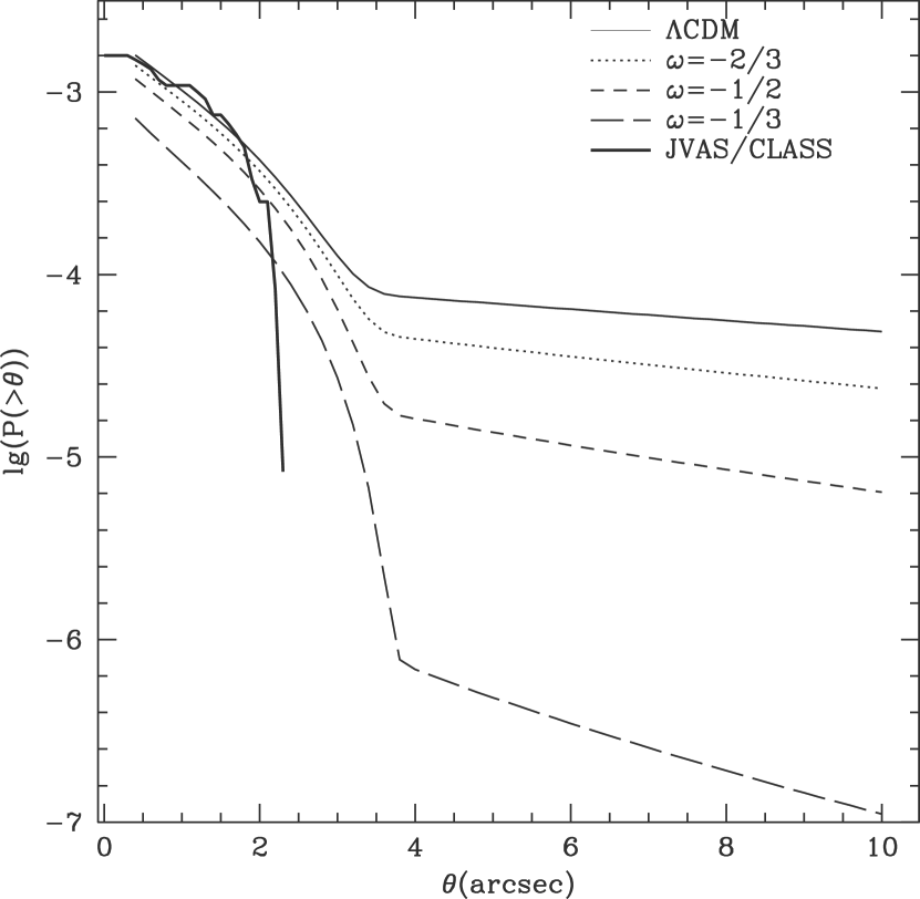
Figure 1: Predicted lensing probability with image separation $>\theta$ in cosmological models with different equation of state $\omega$. The lenses follow the mass function of Jenkins et al. (2001) and are modeled as SIS for $M<1.5\times 10^{13}h^{-1}M_{\odot}$ and as NFW halos with the concentration parameter $c(M,z)=9(1+z)^{-1}(M/M_{*})^{-0.13}$, where $M_{*}=1.5\times 10^{13}h^{-1}M_{\odot}$ (Bullock et al. 2001). The histogram represents the survey results of JVAS/CLASS.

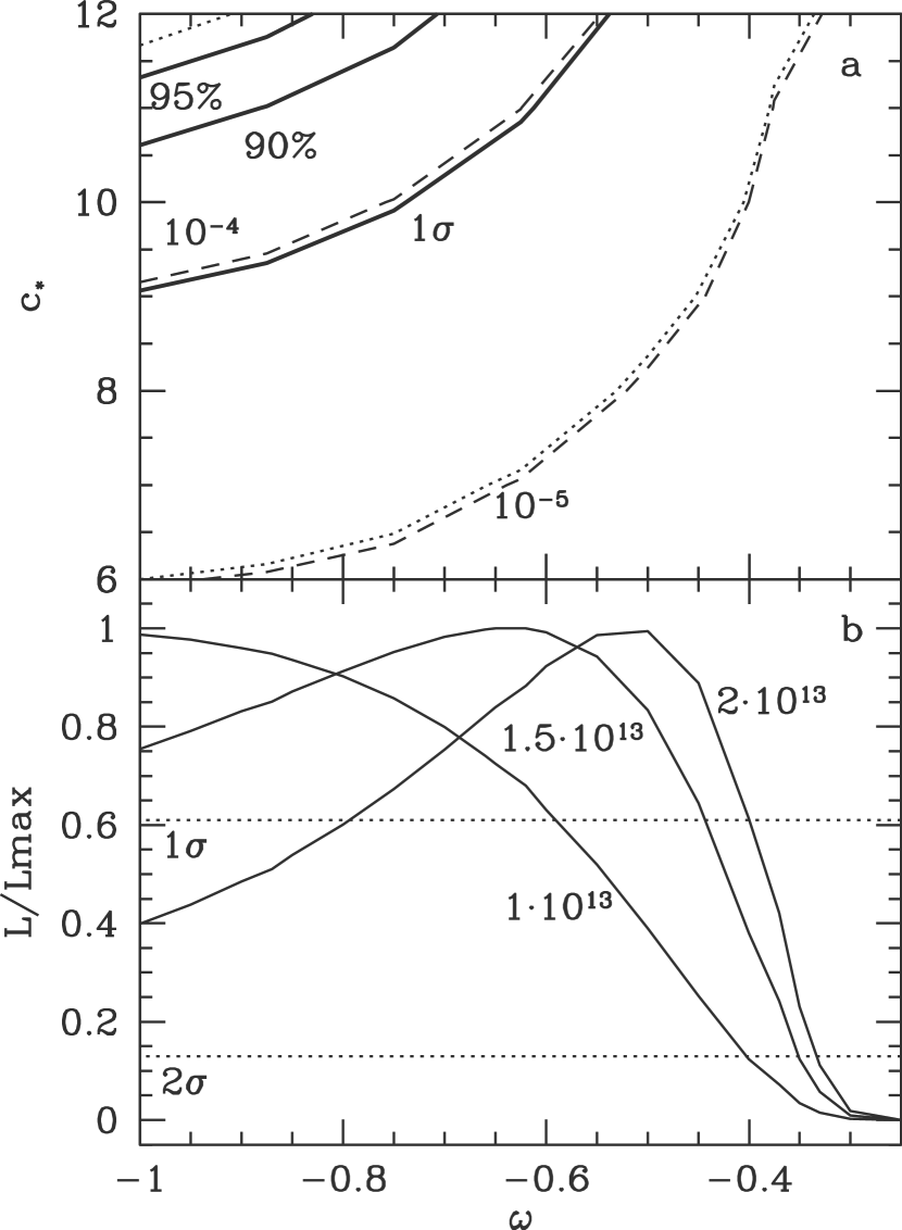
Figure 2: a) Wide separation lensing probability $P(>4^{\prime\prime})$ as a function of the equation of state $\omega$ and the halo concentration $c_{*}$, where $c(M,z)=c_{*}(1+z)^{-1}(M/M_{*})^{-0.13}$. Thick contours are various confidence upper limits for JVAS/CLASS, which has detected zero lenses with $\theta>4^{\prime\prime}$. (Upper-left corner is excluded.) Dotted contours represent the $1\sigma$ confidence levels that would be imposed if one large separation lens were discovered. Dashed contours are for $P(>4^{\prime\prime})=10^{-4}$ and $10^{-5}$. b) Likelihood curves for detecting 18 lenses from 12000 sources (found in JVAS/CLASS) for three different cooling masses. The dotted lines represent the $1\sigma$ and $2\sigma$ confidence levels. Models with $\omega\gtrsim-0.4$ are disfavored at $2\sigma$.

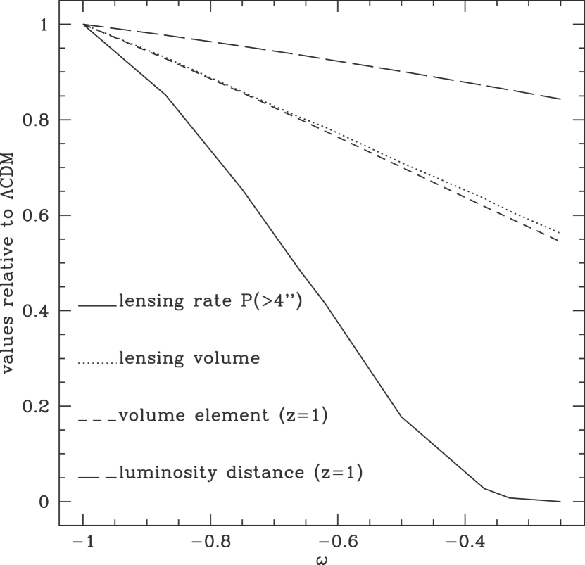
Figure 3: Ratio of four quantities in an $\omega>-1$ model relative to the $\Lambda\rm{CDM}$ model: the lensing probability $P(>4^{\prime\prime})$ for wide separation systems, the effective lensing volume element $(D_{l}D_{ls}/D_{s})^{2}\,dr/dz$ (at $z_{l}=0.5$ and $z_{s}=1.5$), the volume element $dV/dzd\Omega$, and the luminosity distance $d_{L}$ (both at $z=1$).

References

- (1)
- (2) Browne, I.W.A., & Myers, S.T. 2000, proceedings of IAU Symposium 201
- (3)
- (4) Browne, I.W.A., et al. 2001, MNRAS, submitted
- (5)
- (6) Bryan, G.L., & Norman, M.L. 1998, ApJ, 495, 80
- (7)
- (8) Bullock, J.S. et al. 2001, MNRAS, 321, 559
- (9)
- (10) Caldwell, R.R., Dave, R., & Steinhardt, P.J. 1998, Phys. Rev. Lett., 80, 1582
- (11)
- (12) Cohn, J.D., Kochanek, C.S., McLeod, B.A., & Keeton, C.R. 2001, ApJ, 554, 1216
- (13)
- (14) Cooray, A.R., & Huterer, D. 1999, ApJ, 513, L95
- (15)
- (16) David, L.P., Jones, C., & Forman, W. 1995, ApJ, 445, 578
- (17)
- (18) Frieman, J. A., Hill, C.T., Stebbins, A., & Waga, I. 1995, Phys. Rev. Lett.75, 2077
- (19)
- (20) Henstock, D., Browne, I., Wilkinson, P., & McMahon, R. 1997, MNRAS, 290, 380
- (21)
- (22) Jenkins, A. et al. 2001, MNRAS, 321, 372
- (23)
- (24) Keeton, C. 1998, thesis
- (25)
- (26) Keeton, C., & Madau, P. 2001, ApJ, 549, L25
- (27)
- (28) King, L., Browne, I., Marlow, D., Patnaik, A., & Wilkinson, P. 1999, MNRAS, 307, 225
- (29)
- (30) Kochanek, C.S. 1995, ApJ, 445, 559
- (31)
- (32) Kochanek, C.S. 1996, ApJ, 466, 638
- (33)
- (34) Kochanek, C. S., & White, M. 2001, ApJ, in press (astro-ph/0102334)
- (35)
- (36) Li, L.-X., & Ostriker, J.P. 2001, ApJ, in press (astro-ph/0010432)
- (37)
- (38) Ma, C.-P., Caldwell, R.R., Bode, P., & Wang, L. 1999, ApJ, 521, L1
- (39)
- (40) Maoz, D., & Rix, H.-W. 1993, ApJ, 416, 425
- (41)
- (42) Marlow, D., Rusin, D., Jackson, N., Wilkinson, P., Browne, I., & Koopmans, L. 2000, AJ, 119
- (43)
- (44) Myers, S.T., et al. 1999, AJ, 117, 2565
- (45)
- (46) Myers, S.T., et al. 2001, AJ, submitted
- (47)
- (48) Narayan, R., & White, S.D.M. 1988, MNRAS, 231, 97p
- (49)
- (50) Navarro, J.F., Frenk, C.S., & White, S.D.M. 1997, ApJ, 490, 493
- (51)
- (52) Netterfield, C.B. et al. 2001, ApJ, submitted (astro-ph/0104460)
- (53)
- (54) Newman, J., & Davis, M. 2000, ApJ, 534, L11
- (55)
- (56) Patnaik, A.R., Browne, I.W.A., Wilkinson, P.N., & Wrobel, J.M. 1992, MNRAS, 254, 655
- (57)
- (58) Percival, W.J., et al. 2001, MNRAS, submitted (astro-ph/0105252)
- (59)
- (60) Perlmutter, S. et al. 1999, ApJ, 517, 565
- (61)
- (62) Perlmutter, S., Turner, M., & White, M. 1999, Phys. Rev. Lett., 83, 670
- (63)
- (64) Phillips, P.M., Browne, I.W.A., Wilkinson, P.N., & Jackson, N.J. 2000, proceedings of IAU Symposium 201 (astro-ph/0011032)
- (65)
- (66) Porciani, C., & Madau, P. 2000, ApJ, 532, 679
- (67)
- (68) Press, W.H., & Schechter, P. 1974, ApJ, 187, 425
- (69)
- (70) Pryke, C. et al. 2001, ApJ, submitted (astro-ph/0104490)
- (71)
- (72) Riess, A.G. et al. 1998, AJ, 116, 1009
- (73)
- (74) Riess, A.G. et al. 2001, ApJ, in press (astro-ph/0104455)
- (75)
- (76) Rix, H.-W., de Zeeuw, P., Cretton, N., van der Marel, R., & Carollo, C. 1997, ApJ, 488, 702
- (77)
- (78) Rusin, D., & Ma, C.-P. 2001, ApJ, 549, L33
- (79)
- (80) Rusin, D., & Tegmark, M. 2001, ApJ, 553, 709
- (81)
- (82) Schneider, P., Ehlers, J., & Falco, E. E. 1992, Gravitational Lenses (Berlin: Springer-Verlag)
- (83)
- (84) Takahashi, R., & Chiba, T. 2001, astro-ph/0106176
- (85)
- (86) Turner, E. L., Ostriker, J. P., & Gott, J. R. 1984, ApJ, 284, 1
- (87)
- (88) Turner, M. S., & White, M. 1997, Phys. Rev. D56, R4439
- (89)
- (90) Turner, M. S. 2001, astro-ph/0108103
- (91)
- (92) Wang, L., Caldwell, R.R., Ostriker, J. P, & Steinhardt, P. J. 2000, ApJ, 530, 17
- (93)
- (94) Wyithe, J. S. B., Turner, E. L., & Spergel, D. N. 2001, ApJ, 555, 504
- (95)