Photon Folding for Imaging in Non-Focusing Telescopes

Abstract

We present a new technique – photon folding – for imaging in non-focusing telescopes. Motivated by the epoch-folding method in timing analysis, the photon folding technique directly provides the statistical significance of signals in images, using projection matrices. The technique is very robust against common imaging problems such as aspect errors and non-uniform background. The technique provides a deterministic recursive algorithm for improving images, which can be implemented on-line. Higher-order photon folding technique allows a systematic correction for coding noises, which is suitable for studying weak sources in the presence of highly variable strong sources. The technique can be applied to various types of non-focusing telescopes such as coded-aperture optics, rotational collimators or Fourier grid telescopes.

keywords: coded-aperture system, modulation collimator, Fourier grid telescope, epoch-folding method

1 Introduction

Localization or image reconstruction of astrophysical sources at hard X-ray/$\gamma$-ray energies by non-focusing telescopes, such as a coded-aperture system or modulation collimator, has always been a challenging topic. This is largely due to an intrinsically low signal-to-noise ratio (SNR) in non-focusing systems compared to focusing instruments [1]. Consequently, the next generation hard X-ray telescopes, such as HEFT or Constellation-X/HXT, push focusing optics up to energies as high as 100 keV [2, 3]. In order to study astrophysical sources at energies above $\sim$ 100 keV, however, we still have to rely on some sort of non-focusing schemes for the time being [4, 5].

For example, gamma-ray bursts, one of the long-standing mysteries in astronomy, usually have about 90% of their measured flux in the energy range from $\sim$ 100 keV to a few MeV. Their secret is expected to be solved or at least resolved greatly by non-focusing instruments such as Swift in the near future [6]. The fast, accurate localization of bursts by non-focusing optics is required to guarantee effective multi-frequency follow-up observations, which may be important for understanding the physics of the bursts, as demonstrated in recent BeppoSAX observations [5].

There are many techniques for reconstructing images in non-focusing telescopes. For example, in coded-aperture systems, two types of methods are largely used – correlation and inversion methods. Both methods are subject to either coding noise or quantum noise, which leads to spurious fluctuations in images. In order to improve the quality of images, a lot of different techniques are also employed such as pixon or maximum entropy method (MEM) [7, 8]. These methods are computationally intensive and, quite often, requires extensive control over somewhat uncertain parameters in order to produce satisfactory results.

More importantly, in the case of applying non-linear refinement algorithms like pixon or MEM on images reconstructed by correlation or inversion methods, time-independent point spread functions (maybe position dependent) are usually used. Therefore, without prior knowledge of the sources intensity change, it is rather difficult to deal with variable sources when the sources in the FOV have apparent movements due to motions of telescope relative to the sky.

Here we introduce a new method – photon folding – for imaging in non-focusing optics. The basic idea of photon folding is motivated by the well-known epoch-folding method in timing analysis, which is a powerful, yet very simple procedure for finding periodicities in data [9, 10]. The photon-folding method provides a natural way to assess the statistical significances of images, which is inherited from the epoch-folding method. Our technique uses only projection matrices and can be applied to various types of non-focusing optics. The technique is flexible enough to include corrections for aspect errors and non-uniform background.

The criterion given by the photon folding technique allows a recursive method for improving images without human supervision of any parameters, and thus it can be implemented as on-line data processing. In practice, the relative orientation between telescopes and astrophysical sources continues to change during observations and the intensity of sources may also vary. In such cases, recursive methods cannot always effectively extract the location or intensity of a certain source particularly in the presence of highly variable stronger sources. High-order photon folding provides a systematic correction for coding noises in such cases beyond what conventional methods can provide.

We demonstrate the idea using a two-dimensional coded-aperture system. The technique can be readily generalized to other systems such as modulation collimators.

2 Photon Folding Theory

2.1 Basic Concept

Consider a typical coded-aperture telescope with a uniform background, where projection matrix $P_{ij}$ can have either 0 (closed) or 1 (open mask element). A source $s_{j}$ from direction $j$ in the sky can generate counts $h_{i}$ at bin $i$ in the detector as

$$h_{i} =\sum_{j}P_{ij}s_{j}+b_{i},$$ (1)

where $b_{i}$ represents the background count at bin $i$ in the detector ($H=\Sigma h_{i}$). We use index symbol $i$ for detector bins and all the other index symbols ($j$,$k$,$l$) represent sky coordinates. Usually the expected image $\hat{s}_{j}$ is reconstructed as

$$\hat{s}_{j} =\sum_{i}G_{ji}h_{i},$$ (2)

where $G_{ji}$ is a reconstruction matrix, usually given by inversion or correlation methods.

The epoch-folding method in timing analysis searches for any deviation in the data from a flat distribution. Like the $\chi^{2}$-test in the epoch-folding method, we can define $\xi^{2}$ as

$$\xi^{2} =\sum_{i}\frac{\left(h_{i}-\bar{h}\right)^{2}}{\bar{h}},$$ (3)

where $\bar{h}$ is the average of $h_{i}$. In a typical coded-aperture system whose overall transparency is close to 0.5, $\xi^{2}$ from a point source has the largest value while $\xi^{2}$ from a flat field observation is close to a minimum. Consequently, the above $\xi^{2}$ indicates the presence of sources within the field of view (FOV), but it cannot reveal the location of the sources.

In general, the fraction ($\rho$) of open mask elements seen by the detector depends on the direction in the sky, i.e.

$$\rho\equiv\rho_{j}=\sum_{i:P_{ij}=1}\frac{1}{M}=\sum_{i}\frac{P_{ij}}{M},$$ (4)

where $M$ is the number of detector pixels. We can also define $\alpha_{j}$, the fraction of detected photons which can originate from direction $j$ in the sky,

$$\alpha_{j} =\sum_{i:P_{ij}=1}\frac{h_{i}}{H}=\sum_{i}\frac{h_{i}P_{ij}}{H}.$$ (5)

For a given direction in the sky at any moment, one can divide the detector space into two separate regions; the region that can have source photons from the given direction and the other region that is shadowed by the mask (Fig. 1). If there is no source within the FOV, the ratio of the total counts in these two regions will be simply the ratio of open/closed mask elements, i.e. $\alpha_{j}\sim\rho_{j}$. If there is an appreciable source located at the given direction, $\alpha_{j}>\rho_{j}$. The difference of $\alpha_{j}$ and $\rho_{j}$ indicates the probability of having a source at the given direction in the sky.

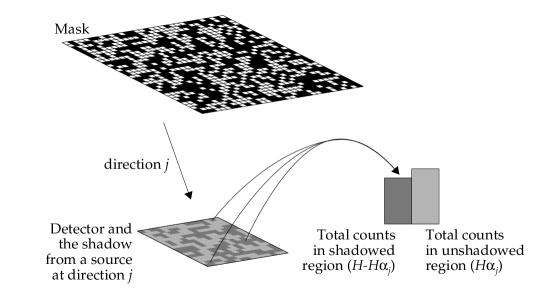
Figure 1: Illustration of photon folding: for a given direction in the sky, the detected photons are folded into two regions – shadowed/unshadowed.

For the direction $j$ in the sky, by folding detected photons into the two regions (Fig. 1), we define $\xi^{2}_{j}$ of the photon folding like the $\chi^{2}$-test in the epoch folding method as

$$\xi^{2}_{j} =\frac{\left(H\alpha_{j}-H\rho_{j}\right)^{2}}{H\rho_{j}}+\frac{\big{(}H(1-\alpha_{j})-H(1-\rho_{j})\big{)}^{2}}{H(1-\rho_{j})}$$

$$=H\frac{\left(\alpha_{j}-\rho_{j}\right)^{2}}{(1-\rho_{j})\rho_{j}}.$$ (6)

In the absence of sources, if $H\alpha_{j}$ and $H(1-\alpha_{j})$ are governed by a normal distribution, the $\xi^{2}_{j}$ of the photon folding follows $\chi^{2}_{2-1}$ statistics. When $p_{1}$ is the probability density of $\chi^{2}$ statistics with one degree of freedom, the probability ($Q_{1}$) of having $\chi^{2}$ greater than $\eta$ is given as

$$Q_{1}(\chi^{2}_{1}\geq\eta) =\int^{\infty}_{\eta}p_{1}(\chi^{2})d\chi^{2},$$ (7)

and then, the confidence level $C$ is related to $Q_{1}$ as,

$$1-\frac{C}{100} =KQ_{1}(\chi^{2}_{1}\geq\eta),$$ (8)

where $K$ is the number of sky bins.

If there is only one source ($s_{j}$) within the FOV, the reconstructed image ($\hat{s}_{j}$) can be directly calculated from $\alpha_{j}$ as

$$\hat{s}_{j}=\frac{H(\alpha_{j}-\rho_{j})}{M(1-\rho_{j})\rho_{j}} =s_{j},$$ (9)

The above formula for $\hat{s}_{j}$ by photon folding is similar to unbiased balanced correlation [11] and becomes identical to the cross correlation method [12] when $P_{ij}$ can have only 0 or 1 and there is only one time bin. For the uniformly redundant array (URA) systems where $\rho_{j}=\rho$, the above formula reduces to the balanced correlation method where $G_{ji}$ is given by

$$G_{ji}=\frac{P_{ij}-\rho}{1-\rho}.$$ (10)

This is not surprising since photon folding searches for a deviation from a flat background distribution similar to the epoch folding method, and the balanced correlation is optimized to cancel out a flat background in the detector.

The immediate advantage of the photon folding is that photon folding provides the statistical significance of signals in images without additional calculations of variances. That is, from Eq. (6) and (9),

$$\frac{\mbox{$\xi^{2}_{j}$}\ }{M^{2}(1-\rho_{j})\rho_{j}}= \frac{\hat{s}_{j}^{2}}{H},$$ (11)

which is similar to the case of focusing optics where the strength of signals in images directly indicates the significance of the signals. Now we derive a generalized photon folding formula which can account for aspect errors and non-uniform background.

2.2 Generalization

For a given direction ($j$) in the sky and for a given time bin ($t$), the detector space can be ranked by the effective transparency through collimators, mask elements, detector efficiency, etc. One can assign this transparency to the projection matrix, which can now have any value from 0 to 1. Thus, in general, the projection matrix $P_{ij}$ can be defined as

$$P_{ij}(t) =0\dots\delta\dots 1,$$ (12)

where $\delta$ is a boundary threshold between shadowed/unshadowed regions. Let $K$, $M$ and $T$ be the total number of bins in sky, detector and time bin respectively ($T$ could be the total duration of the observation when the duration of time bins varies).

Now, we assume that the detector background is known to follow a pattern $\bar{b}_{i}(t)$, which can be estimated by flat-field observations or on-source observation of weak sources. The detected counts $h_{i}(t)$ are given as

$$h_{i}(t) =\sum_{j}P_{ij}(t)s_{j}(t)+b_{i}(t),$$

$$H(t) =\sum_{i}h_{i}(t),$$ (13)

where $b_{i}(t)$ is the actual background counts at detector bin $i$ and at time bin $t$.

For an arbitrary quantity $x_{i}(t)$ in time bin $t$ and detector bin $i$, we define the following quantities.

$$X(t) =\sum_{i}x_{i}(t),$$

$$\lambda_{j_{1}\dots j_{n}:l_{1}\dots l_{n}}[x_{i}(t),t] =\frac{1}{X(t)}\sum_{i:P_{ij_{1}}(t)\geq\delta,\atop\dots P_{ij_{n}}(t)\geq\delta}x_{i}(t)P_{il_{1}}(t)\cdots P_{il_{n}}(t),$$

$$\lambda_{j^{\prime}_{1}\dots j_{n}:l_{1}\dots l_{n}}[x_{i}(t),t] =\frac{1}{X(t)}\sum_{i:P_{ij_{1}}(t)<\delta,\atop\dots P_{ij_{n}}(t)\geq\delta}x_{i}(t)P_{il_{1}}(t)\cdots P_{il_{n}}(t),$$ (14)

where the prime (^′) notation is used to represent a complementary region. For example,

$$\lambda_{jk:l}[x_{i}(t),t]+\lambda_{j^{\prime}k:l}[x_{i}(t),t] =\lambda_{k:l}[x_{i}(t),t].$$ (15)

We introduce $\lambda$ to simplify the following definitions of $\alpha$, $\beta$, and $\rho$ and their explicit definitions are given in the appendix. In terms of $\lambda$, we define

$$\alpha_{j_{1}\dots j_{n}}(t) =\frac{\displaystyle\lambda_{j_{1}\dots j_{n}:}[h_{i}(t),t]}{\lambda_{j_{1}\dots j_{n-1}:}[h_{i}(t),t]},$$

$$\beta_{j_{1}\dots j_{n}}(t) =\frac{\lambda_{j_{1}\dots j_{n}:}[\bar{b}_{i}(t),t]}{\lambda_{j_{1}\dots j_{n-1}:}[\bar{b}_{i}(t),t]},$$

$$\rho_{j_{1}\dots j_{n}:l_{1}\dots l_{n}}(t) =\frac{\lambda_{j_{1}\dots j_{n}:l_{1}\dots l_{n}}[1,t]}{\lambda_{j_{1}\dots j_{n-1}:}[1,t]}.$$ (16)

The above notation allows an intuitive description of the complicated calculations. It should be noted that here $\beta_{...}(t)$ and $\rho_{...}(t)$ can be pre-programmed or pre-calculated. Again in order to simplify the notation, we introduce the sum on time bins as

$$\{X\} =\sum_{t}X(t).$$ (17)

Then, the $\xi^{2}_{j}$ of photon folding is defined as

$$\xi^{2}_{j} =\frac{\displaystyle\big{\{}H\alpha_{j}-H\beta_{j}\big{\}}^{2}}{\displaystyle\big{\{}H\beta_{j}\big{\}}}+\frac{\displaystyle\big{\{}H\alpha_{j^{\prime}}-H\beta_{j^{\prime}}\big{\}}^{2}}{\displaystyle\big{\{}H\beta_{j^{\prime}}\big{\}}}$$

$$=\frac{\displaystyle\big{\{}H\big{\}}\big{\{}H(\alpha_{j}-\beta_{j})\big{\}}^{2}}{\displaystyle\big{\{}H\beta_{j}\big{\}}\big{\{}H(1-\beta_{j})\big{\}}}.$$ (18)

The first-order reconstructed image $\hat{s}_{j}$ is given as

$$\frac{\{\hat{s}_{j}\}}{T} =\frac{\displaystyle\big{\{}H(\alpha_{j}-\beta_{j})\big{\}}}{\big{\{}M(\rho_{j:j}-\rho_{:j}\beta_{j})\big{\}}}.$$ (19)

In the above formula the aspect errors are handled by using a proper $P_{ij}(t)$ at each time bin and the non-uniformity is handled by $\beta_{j}(t)$. The formula does not require an estimation of the overall background level to remove the background pattern. One can express the reconstructed image $\hat{s}_{j}$ in terms of the true signal counts $s_{j}$ as

$$\frac{\{\hat{s}_{j}\}}{T} =\frac{\big{\{}s_{j}(\rho_{j:j}-\rho_{:j}\beta_{j})\big{\}}}{\big{\{}\rho_{j:j}-\rho_{:j}\beta_{j}\big{\}}}+\sum_{k\neq j}\frac{\big{\{}s_{k}(\rho_{j:k}-\rho_{:k}\beta_{j})\big{\}}}{\big{\{}\rho_{j:j}-\rho_{:j}\beta_{j}\big{\}}}.$$ (20)

The second term in the above formula is the coding noise of the system.

3 Refinements

Here we study two refinement procedures of photon folding for suppressing coding noise. The first technique, recursive folding, is similar to conventional recursive methods (e.g. IROS) [11], which successively remove the side lobes – coding noise of strong sources. The second technique, high-order folding, represents a novel approach to the coding-noise problem.

3.1 Recursive Folding

A simple way to remove coding noise is to photon fold recursively. For a given confidence $C$, the $\xi^{2}_{j}$ of photon folding will determine detections of signals in the image based on Eq. (8). Since the signal $\hat{s}_{j}$ is expected to generate counts $\hat{h}_{i}$, we replace $h_{i}$ by

$$h_{i} \leftarrow h_{i}-\hat{h}_{i},\ \ \ \mbox{ where }$$

$$\hat{h}_{i} =\sum_{j}\{\{\hat{s}_{j}\}P_{ij}\}/T,$$ (21)

and repeat the procedure until no excess $\xi^{2}_{j}$ is found for the given confidence. The final image is the sum of $\hat{s}_{j}$ at all the recursion steps and the residual. This is very similar to many other recursive methods. Recursive folding is deterministic since it does not require an initial guess and has a clear stopping point given by the confidence level. This feature is missing in some image refinement procedures such as MEM.

The above formula assumes that the source intensity and detector background level are constant during the observation, or that the detector orientation relative to the sky is fixed. In practice, this is rarely the case. Without information on source intensity/background history, the recursive method does not provide an effective correction to coding noise. In this sense, the recursive technique is not a true solution for coding noise. Now we study another approach to the coding noise problem.

3.2 High-Order Folding

Consider the case where there is only one strong source ($s_{l}$) within the FOV. Given the detection of this source by regular photon folding, one can again apply photon folding only in the detector space shadowed by the mask from direction $l$ in the sky. Since in the shadowed region there is no contribution from source photons at direction $l$, this second-order photon folding will provide an image which is free of the coding noise from the source in direction $l$.

We redefine the total counts and the total number of detector bins only in the shadowed region for the given sky direction $l$ as following:

$$H_{l^{\prime}}(t) =H(t)\alpha_{l^{\prime}}(t),$$

$$M_{l^{\prime}}(t) =\sum_{i:P_{il}(t)<\delta}1.$$ (22)

$\xi^{2}_{l^{\prime}j}$ for the second-order photon folding will be given by

$$\xi^{2}_{l^{\prime}j}\Big{|}_{j\neq l} =\frac{\displaystyle\big{\{}H_{l^{\prime}}\alpha_{l^{\prime}j}-H_{l^{\prime}}\beta_{l^{\prime}j}\big{\}}^{2}}{\displaystyle\big{\{}H_{l^{\prime}}\beta_{l^{\prime}j}\big{\}}}+\frac{\displaystyle\big{\{}H_{l^{\prime}}\alpha_{l^{\prime}j^{\prime}}-H_{l^{\prime}}\beta_{l^{\prime}j^{\prime}}\big{\}}^{2}}{\displaystyle\big{\{}H_{l^{\prime}}\beta_{l^{\prime}j^{\prime}}\big{\}}}$$

$$=\frac{\displaystyle\big{\{}H_{l^{\prime}}\big{\}}\big{\{}H_{l^{\prime}}(\alpha_{l^{\prime}j}-\beta_{l^{\prime}j})\big{\}}^{2}}{\displaystyle\big{\{}H_{l^{\prime}}\beta_{l^{\prime}j}\big{\}}\big{\{}H_{l^{\prime}}(1-\beta_{l^{\prime}j})\big{\}}}.$$ (23)

The image by the second-order photon folding will be given as

$$\frac{\{\hat{s}_{l^{\prime}j}\}_{j\neq l}}{T} =\frac{\displaystyle\big{\{}H_{l^{\prime}}(\alpha_{l^{\prime}j}-\beta_{l^{\prime}j})\big{\}}}{\big{\{}M_{l^{\prime}}(\rho_{l^{\prime}j:j}-\rho_{l^{\prime}:j}\beta_{l^{\prime}j})\big{\}}}.$$ (24)

The above two formulae are exactly the same as Eq. (18) and (19) except for an additional index $l^{\prime}$. The complete expression for an arbitrary order of photon folding can be written by simply adding the additional indices for each term (refer to Appendix). In terms of true signal counts $s_{j}$,

$$\frac{\{\hat{s}_{l^{\prime}j}\}_{j\neq l}}{T} =\frac{\big{\{}s_{j}(\rho_{l^{\prime}j:j}-\rho_{l^{\prime}:j}\beta_{l^{\prime}j})\big{\}}}{\big{\{}\rho_{l^{\prime}j:j}-\rho_{l^{\prime}:j}\beta_{l^{\prime}j}\big{\}}}+\sum_{k\neq j,l}\frac{\big{\{}s_{k}(\rho_{l^{\prime}j:k}-\rho_{l^{\prime}:k}\beta_{l^{\prime}j})\big{\}}}{\big{\{}\rho_{l^{\prime}j:j}-\rho_{l^{\prime}:j}\beta_{l^{\prime}j}\big{\}}}$$

$$\ +\frac{\big{\{}s_{l}(\rho_{l^{\prime}j:l}-\rho_{l^{\prime}:l}\beta_{l^{\prime}j})\big{\}}}{\big{\{}\rho_{l^{\prime}j:j}-\rho_{l^{\prime}:j}\beta_{l^{\prime}j}\big{\}}}.$$ (25)

The second and third term in the above formula represent the coding noise of the system from second-order photon folding. In general, $\rho_{l^{\prime}...:l}$ in the third term keeps the coding noise from the strong source $s_{l}$ very small. For example, in a system with $P_{ij}$ being either 0 or 1, there is no coding noise from $s_{l}$ since $\rho_{l^{\prime}...:l}=0$. When there is a strong point source within the FOV, the above method will provide the best image of weak sources within the FOV regardless of the time dependence of the intensity of the strong source relative to the background level.

There are a few problems in applying the above formula in practical situations. First, although the second-order folding removes the coding noise from the primary strong sources, the coding noise from other weak sources is larger in the second-order folding than in the regular photon folding since the second-order folding utilizes only part of the mask pattern or detector space. Such increase of coding noise from weak sources does not guarantee the reduction of the overall coding noises in high-order photon folding.

Second, the above formula might not be suitable for multiple strong sources or an extended object. In the presence of multiple strong sources, one might have to rely on third or higher-order folding involving the shadowed region for all the directions of strong sources. In typical coded aperture systems, $\rho\sim 0.5$, so that there is only $\rho^{n}$ fraction of the detector area for the completely shadowed region from $n$ point sources. That is, the shadowed region for high-order folding runs out quickly as the number of sources increases.

In order to overcome larger coding noise from weak sources in second-order photon folding, the other region – the unshadowed region ($\{\hat{s}_{lj}\}$) by the primary strong sources – should be utilized as well as the shadowed region ($\{\hat{s}_{l^{\prime}j}\}$). If the detector background is uniform, the second-order photon folding in the unshadowed region will provide similar results as in the shadowed region. For example, in the case of the uniform background system with $P_{ij}$ being either 0 or 1, the term in $\{\hat{s}_{lj}\}_{j\neq l}$, equivalent to the third term in Eq. (25), is proportional to $\rho_{lj:l}-\rho_{l:l}\beta_{lj}$ which vanishes.

In general, the images by second-order folding, $\{\hat{s}_{lj}\}_{j\neq l}$ and $\{\hat{s}_{l^{\prime}j}\}_{j\neq l}$ will have substantially reduced contributions from the coding noise of primary strong sources at direction $l$. Both images, however, have larger coding noises from the secondary sources. The best second-order photon-folding image will be a linear combination of these two images, i.e.

$$\gamma\{\hat{s}_{l^{\prime}j}\}+(1-\gamma)\{\hat{s}_{lj}\}.$$ (26)

The optimal $\gamma$ strongly depends on $\delta$, $P_{ij}$, and etc. For a given detection of a strong source by the regular photon folding, the optimal $\gamma$ for the second-order photon folding can be estimated by using only the strong source with constant intensity. In other words, we first calculate $\{\hat{s}^{0}_{l^{\prime}j}\}$,$\{\hat{s}^{0}_{lj}\}$ from $\hat{h}_{i}$ instead of $h_{i}$, where

$$\hat{h}_{i} =\{\{\hat{s}_{l}\}P_{il}\}/T,$$ (27)

and then use the $\gamma$ in Eq. (26), which minimizes

$$\gamma\{\hat{s}^{0}_{l^{\prime}j}\}+(1-\gamma)\{\hat{s}^{0}_{lj}\}.$$ (28)

This procedure is valid when $s_{l}$ is much stronger than $s_{j}$, which is the assumption of this technique. Here once again we assume the constancy of the source intensity in Eq. (27), but due to the terms like $\rho_{l^{\prime}...:l}$ in the coding noise from strong source $s_{l}$, the changes of the source intensity are less serious in the second-order folding than in the recursive method.

Now, we consider the case of multiple strong sources. When $\{s_{l}\}\gg\{s_{j}\}$, the reconstructed images by the regular and second-order folding can be summarized as

$$\{\hat{s}_{j}\} =O(\tau_{j})\{s_{j}\}+\sum_{k\neq j}O(\tau_{k}\epsilon)\{s_{k}\},$$

$$\gamma\{\hat{s}_{l^{\prime}j}\}+(1-\gamma)\{\hat{s}_{lj}\} =O(\tau_{j})\{s_{j}\}+\sum_{k\neq j,l}O(\tau_{k}\epsilon)\{s_{k}\}+O(\tau_{l}\epsilon^{2})\{s_{l}\},$$ (29)

where $\tau$ represents the temporal uniformity of the source with respect to the background level and $\epsilon$ is the size of coding noise. Since the contributions of source $s_{k}|_{k\neq j,l}$ (the second term in the right hand side of the above formula) should be similar in both images from the first-order and second-order folding, we expect that the following formula provides a more reliable estimate for $s_{j}$ in the case of multiple strong sources.

$$\sum_{l\neq j\atop\xi^{2}_{l}>\eta}\Big{(}\gamma\{\hat{s}_{l^{\prime}j}\}+(1-\gamma)\{\hat{s}_{lj}\}\Big{)} -(L-1)\{\hat{s}_{j}\}$$

$$=O(\tau_{j})\{s_{j}\}+\sum_{k\neq j}O(\tau_{k}\epsilon^{2})\{s_{k}\},$$ (30)

where $L$ is the number of sources detected in the first-order photon folding and $\gamma$ is calculated by minimizing

$$\sum_{l\neq j\atop\xi^{2}_{l}>\eta}\gamma\{\hat{s}^{0}_{l^{\prime}j}\}+(1-\gamma)\{\hat{s}^{0}_{lj}\}.$$ (31)

The left hand side of Eq. (30) is expected to reduce the coding noise below that from the first-order image and is less sensitive to the intensity variation of the strong sources compared to the recursive method.

4 Simulations

We demonstrate the photon folding technique on a coded-aperture imaging system. The system consists of 64 $\times$ 64 random mask elements ($P_{ij}$= 0 or 1) and the detector has 32 $\times$ 32 elements.

The first example has four point sources and one extended source within the FOV. Two of the point sources are very strong and the other sources are relatively weak. During the simulated observation we assume that the relative orientation of the mask pattern with respect to the sky has rotated 90 degrees from the first half to the second half of the measurement. This is a somewhat extreme case of the change of telescope orientation relative to the sky during the observation. When reconstructing images, we combine all the data and we assume that the intensity change of the sources during the observation is unknown, i.e. the intensity is assumed to be constant. The aspect system and spatial resolution of the detector are assumed to be perfect.

The upper plots in Fig. 2 show the true sky image and the simulated detector counts. We assume that the detector background exhibits a quadratic spatial dependence, resulting in an enhancement of counts at the edges. Such a pattern is somewhat common and we assume that the pattern is known by previous flat field observations or calibrations.

In Fig. 2, the intensity of sources in the sky did not vary during the simulated observation. The lower three plots show the reconstructed images by regular photon folding, recursive folding, and second-order folding. The regular photon folding, which is equivalent to the cross correlation method in this case, successfully detects the strong sources, but the coding noise of the strong sources buries features of weak sources. The recursive folding presents the best image in this case, and its quality is limited only by random Poisson noise. Second-order folding also reconstructs a decent image which reveals the fine structure of weak sources. The noise in the image by second-order folding is mostly random Poisson noise and coding noise of weak sources.

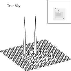
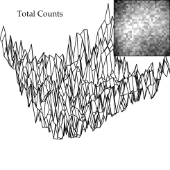
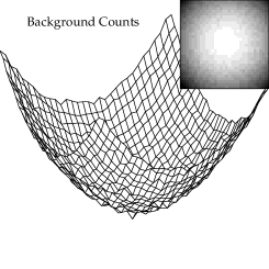
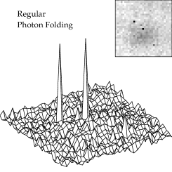
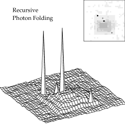
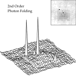
Figure 2: Simulation of steady sources: the upper plots are the simulated sky image, total counts, and background counts in the detector. The lower plots show the reconstructed images by regular photon folding, recursive folding, and second-order folding. The orientation of the telescope relative to the sky has changed 90 degrees from the first to the second half of the observation.

Now, in Fig. 3, we have an extreme case of a more realistic situation. The intensity of two strong sources changed dramatically from the first to the second half of the observation. If the relative orientation between the telescope and the sky did not change, the results would be similar to those in Fig. 2. But here we assume that the relative orientation changed 90 degrees.

Under the assumption of being unaware of the source intensity changes, the bottom plots in Fig. 3 show the three reconstructed images. The recursive method fails to show the fine structure of weak sources. It should be noted that this result is generally true for any type of recursive method without prior information on source intensity changes. On the other hand, the second-order folding produces almost the same image as in the previous case, i.e. only limited by the random Poisson noise and coding noise of weak sources

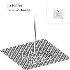
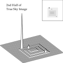
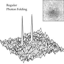
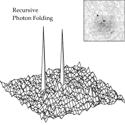
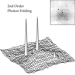
Figure 3: Simulation of variable sources: the upper plots show the true sky image in the first and second half of the observation. The orientation of the telescope relative to the sky has changed 90 degrees from the first to the second half. Reconstructed images by the regular photon folding, recursive folding and second-order photon folding are shown in the lower plots.

In order to see the general performance of the recursive method and the second-order photon folding, we calculate SNRs of a few simple simulations with a flat background pattern. In the following figure, we show the SNR of a point source in four distinct situations (1 $\sigma$ distribution of the simulation results). Each observation consists of two measurements as in the previous example (90 degree offset of the relative orientation).

Fig. 4 (a) shows the case of a steady single source within the FOV. The second-order folding and recursive folding generate images with the maximally allowed SNR, while SNRs from regular folding are limited by coding-noise. In Fig. 4 (b), the source intensity dropped to zero for the second half. While second-order folding performs similarly to the previous cases, the performance of recursive folding is limited by coding noises.

In Fig. 4 (c), there are five steady point sources within the FOV. In this case, the recursive folding produces perfect images, while second-order folding shows its limitation due to incomplete correction of the coding noise from multiple sources. In Fig. 4 (d), there are five variable point sources, and the intensity of three sources drops from maximum to zero and the intensity of the other two rises from zero to maximum from the first to the second half of the observation. It is clear that if there is a change in source intensity, second-order folding is the better choice, while in the case of many multiple steady sources recursive folding is the optimal method.

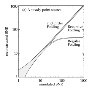
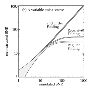
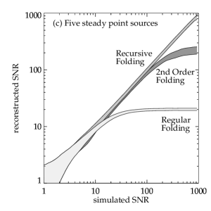
Figure 4: SNRs in various cases: within the FOV, there is (a) a steady point source (b) a variable point source, (c) five steady point sources, and (d) five variable point sources. The overall intensity of each source in multiple-source cases are the same.

5 Discussion

The photon folding and associated techniques can be applied in many non-focusing instruments. Recursive folding and second-order folding are complementary to each other in various realistic situations. Here we discuss some of the fundamental issues.

5.1 Computational Issues

Computational time for regular photon folding is similar to that of the cross correlation method. Since the photon folding automatically takes care of aspect errors and non-uniform background, the overall computational burden for photon folding is similar to regular correlation or inversion techniques.

If we let $N$ be the number of calculations for photon folding, the recursive folding requires $N_{r}N$ calculations where $N_{r}$ is the total number of recursion steps. $N_{r}$ depends on intensity distribution of sources in the FOV. Second-order folding requires $(2N_{s}+1)N$ calculations, where $N_{s}$ is the number of strong sources detected in the regular photon folding. The extra $N$ comes from the estimation of the optimum $\gamma$ for the given detection. Since photon folding does not involve inversion of matrices, this number of calculations is not a problem even for a huge number of sky or detector pixels due to the improvements of modern computing power.

Both recursive and second-order folding can be implemented on-line. While the recursive folding is somewhat straightforward in on-line processing, second-order folding requires more caution. The successful image reconstruction of second-order folding depends on limiting the number ($L$) of sky pixels for the first-order detection and yet including enough of them to remove most of the coding noise. Selecting a few of the strongest sources for the first detection would be adequate for an automatic implementation.

5.2 Recursive vs Second-order folding

These two techniques are somewhat complementary to each other in various situations. Fig. 5 summarizes the simulations in the previous section (Fig. 4) in terms of relative SNR. In Fig. 5, each of the shaded regions represents each case of the simulations in Fig. 4 where simulated SNR is between 50 and 1000. For a given value of the simulated SNR, recursive folding produces better results in the case of many steady sources, while second-order folding does so in the case of variable sources.

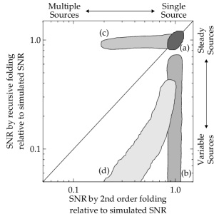
Figure 5: Recursive vs Second-order photon folding: (a) a steady source (b) a variable source, (c) five steady sources, and (d) five variable sources. The $x$-axis is the SNR by second-order photon folding relative to the simulated SNR, and $y$-axis the SNR by recursive folding folding relative to the simulated SNR. Each shaded region represents each of the four cases of simulations in Fig. 4 where simulated SNR is between 50 and 1000.

The second-order photon folding is less robust against aspect errors or non-uniformity of the background than the recursive folding. Having uncorrectable aspect errors is somewhat equivalent to having multiple sources in the FOV. The non-uniform background in the second-order image ($\{\hat{s}_{lj}\}$) from the unshadowed region cannot cancel out in photon folding, depending on the strength of the strong source $s_{l}$ relative to the background level.

5.3 Other variations of photon folding

So far we use only two folded bins – shadowed/unshadowed region – for photon folding. In general, increasing the number of folded bins does not boost SNR. However it may be useful to have more than two folded bins when effective transparencies have more than two distinct values or there are severe non-uniformities in the detector background. One can also utilize higher-order folding beyond second-order, such as $\hat{s}_{l^{\prime}k^{\prime}j}$, $\hat{s}_{l^{\prime}kj}$, etc. Although higher-order foldings are computationally intensive, the use of higher-order folding could remove the limitation of the second-order folding method in multiple strong source cases. Further studies are required to find a proper form of higher-order folding to suppress even more of the coding noise and also new types of optics scheme can be designed to optimize for high-order photon-folding image reconstruction.

5.4 Applications

The photon folding technique is very versatile, and it can be applied to many different types of experiments. Applying the photon-folding method to other non-focusing systems like Fourier grid systems is quite straightforward. In the case of modulation collimator systems, the location of the source is identified by the temporal modulation rather than the spatial modulation in the detector (usually detectors for modulation collimator systems do not require spatial resolution).

For example, consider a typical rotation modulation collimator. For a given direction in the sky, the fraction ($\rho$) of the shadowed area in the detector changes with time. For a given unit rotation and a given direction in the sky, one can rearrange count rates in the order of the fraction ($\rho$) instead of time, and then apply a folding procedure with a necessary amount of binning. This is somewhat similar to regular epoch-folding in timing analysis. The signal from a point source usually fluctuates between a maximum and minimum during the unit rotation. The temporal resolution, relatively finer than the spatial resolution of a typical detector, might allow effective usage of more than two folded-bins in photon folding.

In coded-aperture systems, photon folding may allow use of non-URA mask patterns. For example, EXIST is a coded-aperture, wide field of view survey mission, with a wide energy range ($\sim$ 10 – 600 keV) [4]. Curved mask patterns are being studied for EXIST to utilize maximal available FOV without substantial collimators between the mask and detectors. In order to cover the wide energy range (10 – 600 keV) in EXIST, two scale mask patterns can be used with energy dependent transparency [13]. Such mask patterns may provide additional advantages over conventional mask patterns, but the optimal imaging reconstruction scheme is not yet available. The photon folding technique may be useful for non-conventional mask patterns. Particularly second-order folding is very interesting for EXIST. The high sensitivity of EXIST is likely to result in detection of multiple, possibly variable sources in each field, and second-order folding would allow imaging of the weak sources.

6 Conclusion

A new imaging technique – photon folding – is introduced for non-focusing telescopes. The technique is quite robust against common imaging problems like aspect errors and non-uniform background. Its performance is demonstrated by a two-dimensional coded-aperture system and photon folding can be applied to other types of imaging telescopes. Two refinements of photon folding are presented – recursive and second-order folding. In particular second-order photon folding is suitable for imaging weak sources in the presence of highly variable strong sources regardless of the changes in telescope orientation relative to the sky.

7 Acknowledgement

The author would like to thank C.J. Hailey for valuable comments and discussion.

Appendix A

For the regular photon folding,

$$\alpha_{j}(t) =\frac{\lambda_{j:}[h_{i}(t),t]}{\lambda_{:}[h_{i}(t),t]}=\frac{1}{H(t)}\sum_{i:P_{ij}(t)\geq\delta}h_{i}(t),$$ (32)

which reduces to Eq. (5) when $P_{ij}$ is either 0 or 1 (constant).

$$\beta_{j}(t) =\frac{\lambda_{j:}[\bar{b}_{i}(t),t]}{\lambda_{:}[\bar{b}_{i}(t),t]}=\frac{1}{\bar{B}(t)}\sum_{i:P_{ij}(t)\geq\delta}\bar{b}_{i}(t),$$ (33)

where $\bar{B}(t)=\Sigma\bar{b}_{i}(t)$. For a flat background pattern, $\beta_{j}(t)=\rho_{j:}(t)$.

And

$$\rho_{j:}(t) =\frac{\lambda_{j:}[1,t]}{\lambda_{:}[1,t]}=\frac{1}{M(t)}\sum_{i:P_{ij}(t)\geq\delta}1,$$

$$\rho_{j:j}(t) =\frac{\lambda_{j:j}[1,t]}{\lambda_{:}[1,t]}=\frac{1}{\displaystyle M(t)}\sum_{i:P_{ij}(t)\geq\delta}P_{ij}(t),$$

$$\rho_{:j}(t) =\frac{\lambda_{:j}[1,t]}{1}=\frac{1}{M(t)}\sum_{i}P_{ij}(t).$$ (34)

If $P_{ij}(t)$ is either 0 or 1, $\rho_{:j}(t)=\rho_{j:j}(t)=\rho_{j:}(t)$.

Now, for second-order photon folding,

$$\alpha_{lj}(t) =\frac{\lambda_{lj:}[h_{i}(t),t]}{\lambda_{l:}[h_{i}(t),t]}$$

$$=\Bigg{[}\frac{\displaystyle 1}{H(t)}\sum_{i:P_{il}(t)\geq\delta,\atop P_{ij}(t)\geq\delta}h_{i}(t)\Bigg{]}\Bigg{[}\displaystyle\frac{1}{H(t)}\sum_{i:P_{il}(t)\geq\delta}h_{i}(t)\Bigg{]}^{-1}$$

$$=\frac{\displaystyle 1}{\displaystyle H(t)\alpha_{l}(t)}\sum_{i:P_{il}(t)\geq\delta,\atop P_{ij}(t)\geq\delta}h_{i}(t)=\frac{1}{H_{l}(t)}\sum_{i:P_{il}(t)\geq\delta,\atop P_{ij}(t)\geq\delta}h_{i}(t).$$ (35)

Likewise,

$$\beta_{lj}(t) =\frac{1}{\bar{B}_{l}(t)}\sum_{i:P_{il}(t)\geq\delta,\atop P_{ij}(t)\geq\delta}\bar{b}_{i}(t)$$

$$\rho_{lj:}(t) =\frac{1}{M_{l}(t)}\sum_{i:P_{il}(t)\geq\delta,\atop P_{ij}(t)\geq\delta}1,$$

$$\rho_{lj:j}(t) =\frac{1}{\displaystyle M_{l}(t)}\sum_{i:P_{il}(t)\geq\delta,\atop P_{ij}(t)\geq\delta}P_{ij}(t),$$

$$\rho_{l:j}(t) =\frac{1}{M_{l}(t)}\sum_{i:P_{il}(t)\geq\delta}P_{ij}(t),$$ (36)

where

$$\bar{B}_{l}(t) =\bar{B}(t)\beta_{l}(t),$$

$$M_{l}(t) =\sum_{i:P_{il}(t)\geq\delta}1.$$ (37)

In $\alpha_{l^{\prime}j}(t)$, $\beta_{l^{\prime}j}(t)$, $\rho_{l^{\prime}j:}(t)$, $\rho_{l^{\prime}j:j}(t)$ and $\rho_{l^{\prime}:j}(t)$, the summation condition, $P_{il}(t)\geq\delta$, in the above equations will be replaced by $P_{il}(t)<\delta$. Therefore, they satisfy the followings relations.

$$\alpha_{lj}(t)+\alpha_{lj^{\prime}}(t) =1,$$

$$\beta_{lj}(t)+\beta_{lj^{\prime}}(t) =1.$$ (38)

The complete expression for an arbitrary order of photon folding can be written simply by keeping additional indices in front of each term.

$$\xi^{2}_{l_{1}...l_{n}j}\Big{|}_{j\neq l_{1}...l_{n}} =\frac{\displaystyle\big{\{}H_{l_{1}...l_{n}}\big{\}}\big{\{}H_{l_{1}...l_{n}}(\alpha_{l_{1}...l_{n}j}-\beta_{l_{1}...l_{n}j})\big{\}}^{2}}{\displaystyle\big{\{}H_{l_{1}...l_{n}}\beta_{l_{1}...l_{n}j}\big{\}}\big{\{}H_{l_{1}...l_{n}}(1-\beta_{l_{1}...l_{n}j})\big{\}}},$$

$$\frac{\{\hat{s}_{l_{1}...l_{n}j}\}_{j\neq l_{1}...l_{n}}}{T} =\frac{\displaystyle\big{\{}H_{l_{1}...l_{n}}(\alpha_{l_{1}...l_{n}j}-\beta_{l_{1}...l_{n}j})\big{\}}}{\big{\{}M_{l_{1}...l_{n}}(\rho_{l_{1}...l_{n}j:j}-\rho_{l_{1}...l_{n}:j}\beta_{l_{1}...l_{n}j})\big{\}}}.$$ (39)

References

- [1] E. E. Fenimore, “Coded aperture imaging: predicted performance of uniformly redundant arrays,” Appl. Opt. 17, 3562–3570 (1978).
- [2] C. J. Hailey, S. Abdali, F. E. Christensen, W. W. Craig, T. R. Decker, F. A. Harrison, and M. Jimenez-Garate, “Substrates and mounting techniques for the High-Energy Focusing Telescope (HEFT),” In Proc. SPIE 3114: EUV, X-Ray, and Gamma-Ray Instrumentation for Astronomy VIII (International Society for Optical Engineering, Bellingham Washington, 1997), Vol. 3114, pp. 535–543.
- [3] N. E. White and H. Tananbaum, “The Constellation X-ray Mission,” In IAU Symp. 195: Highly Energetic Physical Processes and Mechanisms for Emission from Astrophysical Plasmas, (Astronomical Society of the Pacific, San Francisco, California, 2000), Vol. 195, pp. 61–68.
- [4] J. E. Grindlay, L. Bildsten, D. Chakrabarty, M. Elvis, A. Fabian, F. Fiore, N. Gehrels, C. Hailey, F. Harrison, D. Hartmann, T. Prince, B. Ramsey, R. Rothschild, G. Skinner, and S. Woosley, “EXIST: A High Sensitivity Hard X-ray Imaging Sky Survey Mission for ISS,” In AIP conference proceedings: The Fifth Compton Symposium (American Institute Of Physics, Melville, New York, 1999), Vol. 510, pp. 784–788.
- [5] F. A. Harrison, J. S. Bloom, D. A. Frail, R. Sari, S. R. Kulkarni, S. G. Djorgovski, T. Axelrod, J. Mould, B. P. Schmidt, M. H. Wieringa, R. M. Wark, R. Subrahmanyan, D. McConnell, P. J. McCarthy, B. E. Schaefer, R. G. McMahon, R. O. Markze, E. Firth, P. Soffitta, and L. Amati, “Optical and Radio Observations of the Afterglow from GRB 990510: Evidence for a Jet,” Astrophys. J. 523, L121–L124 (1999).
- [6] N. Gehrels and Swift Science Team, “Swift - The Next GRB MIDEX Mission,” In American Astronomical Society Meeting, (American Astronomical Society, Washington, DC, Dec, 1999), Vol. 195, #92.08.
- [7] R. C. Puetter and A. Yahil, “The Pixon Method of Image Reconstruction,” In ASP Conf. Ser. 172: Astronomical Data Analysis Software and Systems VIII (Astronomical Society of the Pacific, San Francisco, California, 1999), Vol. 8, pp. 307–316.
- [8] T. R. Metcalf, D. Alexander, N. Nitta, and T. Kosugi, “A Comparison of the MEM and Pixon Algorithms for HXT Image Reconstruction,” In American Astronomical Society, Solar Physics Division Meeting (American Astronomical Society, Washington, DC, May, 1997), Vol. 28, #02.17.
- [9] D. A. Leahy, W. Darbro, R. F. Elsner, M. C. Weisskopf, S. Kahn, P. G. Sutherland, and J. E. Grindlay. “On searches for pulsed emission with application to four globular cluster X-ray sources - NGC 1851, 6441, 6624, and 6712,” Astrophys. J. 266, 160–170 (1983).
- [10] S. Larsson, “Parameter estimation in epoch folding analysis,” Astro. Astrophys. Suppl. 117, 197–201 (1996).
- [11] A. Hammersley, T. Ponman, and G. Skinner, “Reconstruction of images from a coded-aperture box camera,” Nucl. Instr. Meth. A311, 585–594 (1992).
- [12] G. K. Skinner, R. L. Balthazor, J. R. H. Herring, R. M. Rideout, J. Tueller, S. D. Barthelmy and L. M. Bartlett, “A balloon flight test of a coded-mask telescope with a multi-element germanium detector,” Nucl. Instr. Meth. A357, 580–587 (1995).
- [13] G. K. Skinner and J. E. Grindlay, “Coded masks with two spatial scales,” Astron. Astrophys. 276, 673–681 (1993).