Can stellar winds account for temperature fluctuations
in H ii regions?

We compare the rate of kinetic energy injected by stellar winds into the extragalactic H ii region NGC 2363 to the luminosity needed to feed the observed temperature fluctuations. The kinetic luminosity associated to the winds is estimated by means of two different evolutionary synthesis codes, one of which takes into account the statistical fluctuations expected in the Initial Mass Function. We find that, even in the most favorable conditions considered by our model, such luminosity is much smaller than the luminosity needed to account for the observed temperature fluctuations. The assumptions underlying our study are emphasized as possible sources of uncertainty affecting our results.

1 Introduction

The presence of temperature fluctuations in photoionized regions has been a matter of debate since the pioneering work by Peimbert (1967). Although little doubt on their relevance in real nebulae seems possible on observational grounds (see the review by Peimbert 1995), their inclusion in a theoretical framework is still controversial, given both the incompleteness of the present theoretical scenario, and the technical difficulties implied by their inclusion in photoionization models. Plain photoionization theory predicts temperature fluctuations to be very small, mainly due to the steep dependence of the cooling rate on temperature, which implies that their lifetime would be quite short; yet, the existence of a mechanism steadily providing the energy required to feed them is not excluded by this line of reasoning. The importance of the question can be barely overrated given that, if temperature fluctuations turn out to be as big as observations suggest, the present determinations of chemical abundances should be rescaled by as much as +0.5 dex.

For a long time, the only way temperature fluctuations were accounted for in theoretical models was acknowledging the impossibility to reproduce the observed intensity of the most affected lines; see, e.g., Luridiana et al. (1999) for the case of NGC 2363, and Stasińska & Schaerer (1999) for the case of IZw18. Recently, Binette & Luridiana (2000) developed a model to quantify the effect of temperature fluctuations on the ionization and energy balance of nebulae. In the present work, we use their schema to investigate whether the kinetic energy provided by stellar winds could feed the temperature fluctuations observed in NGC 2363. Throughout the paper, by ‘stellar winds’ we generically refer to all those phenomena involving the ejection of mass from stars into the interstellar medium (ISM). Given the age range considered, the only contributors to stellar winds actually included in the calculations are hot stars and Wolf-Rayet stars (WRs).

The structure of the paper is as follows: in Sect. 2 we summarize the relevant properties of NGC 2363. Sect. 3 describes the model used to represent temperature fluctuations in nebulae. In Sect. 4 we estimate the kinetic luminosity of the stellar cluster in NGC 2363, and apply the method of Sect. 3 to determine whether stellar winds could be responsible for the temperature fluctuations observed in NGC 2363. Finally, in Sect. 5 we analyze several possible sources of uncertainty, and in Sect. 6 we summarize the main conclusions.

2 General properties of NGC 2363

NGC 2363 is a giant extragalactic H ii region, located in the south-west end of the irregular galaxy NGC 2366. It is one of the brightest extragalactic H ii regions known, and an ideal subject for our study, since plenty of data are available, both observational and theoretical. Two distinctive knots can be clearly distinguished in the region: throughout this paper, we will always refer to the brightest, youngest knot, often called ‘knot A’.

NGC 2363 has been observed by several groups (e.g., Peimbert et al. 1986; González-Delgado et al. 1994; Izotov et al. 1997), and modeled by Luridiana et al. (1999) and Drissen et al. (2000) among others, while the temperature-fluctuation parameter has been determined by González-Delgado et al. (1994) in both knots.

In the present work, we will assume that both the stellar cluster and the gas nebula of NGC 2363 are well described by the best-fit model of Luridiana et al. (1999), which is a spherical, hollow, radiation-bounded nebula, consisting of two concentric shells of different densities, ionized by a young cluster undergoing an extended burst of star formation. The properties of the model relevant for this work will be described throughout the text.

3 The energy implications of temperature fluctuations

To quantify the energy injection rate needed to fuel temperature fluctuations in a nebula, we follow the model proposed by Binette & Luridiana (2000) and Binette et al. (2001). The first of these two papers contains a detailed description of the method, while we refer to the second for an alternative representation of the results. The model depicts temperature fluctuations as a collection of hot spots, arising above a uniform equilibrium temperature floor, and fed by an unknown heating agent. This representation allows one to compute the average thermal properties of the nebula in the temperature-fluctuation regime, but without having to compute real localized fluctuations, as described below.

3.1 Definition of temperature fluctuations

The amplitude of temperature fluctuations in a nebula is measured by the parameter $t^{2}$, defined as follows (Peimbert 1967):

$$t^{2}={{\int_{V}(T_{\rm e}{\bf(r)}-T_{\rm 0})^{2}N_{\rm e}{\bf(r)}N_{\rm i}{\bf(r)}dV}\over{T_{\rm 0}^{2}\int_{V}N_{\rm e}{\bf(r)}N_{\rm i}{\bf(r)}dV}}$$ (1)

where $T_{\rm e}{\bf(r)}$ is the local electron temperature, $N_{\rm e}{\bf(r)}$ and $N_{\rm i}{\bf(r)}$ are the local values of the electron and ionic density respectively, $V$ is the observed volume, and the average temperature $T_{\rm 0}$ is given by:

$$T_{\rm 0}={{\int_{V}T_{\rm e}{\bf(r)}N_{\rm e}{\bf(r)}N_{\rm i}{\bf(r)}dV}\over{\int_{V}N_{\rm e}{\bf(r)}N_{\rm i}{\bf(r)}dV}}.$$ (2)

Since the temperature of a model H ii region is not spatially constant, temperature fluctuations appear and evolve following the evolution of the ionization field even in the simplest case of a static, pure photoionization nebula; in particular, Pérez (1997) showed that large temperature fluctuations arise during the WR phase, as a consequence of the hardening of the spectrum. Following the definition by Ferland (1996), we will refer to such ‘structural’ temperature fluctuations as $t^{2}_{\rm str}$. Typical $t^{2}_{\rm str}$ values for photoionization models of chemically and spatially homogeneous model nebulae are in the range $0.00\leq t^{2}_{\rm str}\leq 0.02$. The best-fit photoionization model by Luridiana et al. (1999) yields a value $t^{2}_{\rm str}\sim 0.009$.

On the observational side, González-Delgado et al. (1994) find for NGC 2363 the value $t^{2}_{\rm obs}=0.064$ by comparing the Paschen temperature, $T_{\rm e}(Pa)$, to the [O iii] temperature, obtained from the $\lambda 4363/\lambda 5007$ ratio. Even if in this case the formal error on $t^{2}_{\rm obs}$ is quite large (we calculated $\sigma(t^{2}_{\rm obs})=0.045$, mainly due to the large error on $T_{\rm e}(Pa)$), the differences between the model predictions and the observations seem to imply that an extra-heating mechanism, other than photoionization, is at work in most objects, producing an additional $t^{2}_{\rm extra}$ such that $t^{2}_{\rm obs}=t^{2}_{\rm str}+t^{2}_{\rm extra}$. In the case of NGC 2363, we find $t^{2}_{\rm extra}=0.055\pm 0.045$. Note that such value still leaves the door open to the possibility, small but not negligible, that $t^{2}_{\rm extra}=0.00$; however, we assume this not to be the case. In this respect, it is interesting to note that $t^{2}_{\rm obs}=0.098$ in knot B of the same region (González-Delgado et al. 1994). Given the presumed age and metallicity of this region (Luridiana et al. 1999), and assuming the same filling factor as in knot A, we can roughly estimate $t^{2}_{\rm str}=0.02$ (see, e.g., Pérez 1997), yielding $t^{2}_{\rm extra}=t^{2}_{\rm obs}-t^{2}_{\rm str}=0.078$, with an associated error of about $\sigma(t^{2}_{\rm obs})=0.019$.

More generally, even though the errors might be compatible with $t^{2}_{\rm extra}=0$ in individual cases of ionized regions with $t^{2}_{\rm obs}>0$, this is certainly not the case when large samples are considered. As an example, galactic H ii regions and planetary nebulae collectively show higher values, typically around $0.04$ (e.g., Peimbert et al. 1995; Peimbert 1995, and references therein).

The presence of temperature fluctuations inside NGC 2363 bears important cosmological consequences, as it affects the determination of the chemical abundances, lowering the extrapolated primordial helium abundance $Y_{\rm p}$ (e.g., Peimbert et al. 2001a, and references therein). In our case, $t^{2}_{\rm obs}=0.064$ implies a downward change in the helium abundance of NGC 2363 of order 2%, the exact figure depending on which He lines the abundance determination is based on (see also González-Delgado et al. 1994). It is important to note, however, that temperature fluctuations are not the only factor affecting a proper chemical abundance determination, other being, e.g, the ionization structure and the collisional excitation of the hydrogen lines (Stasińska & Izotov 2001; Peimbert et al. 2001b).

3.2 The hot-spot scheme

The overall energy balance in a nebula is described by the following equation:

$$H=G$$ (3)

where $H$ and $G$ are the heating and cooling rates respectively. In a nebula in ionization equilibrium, with no extra-heating sources, the heating is provided by photoionization, and the cooling takes place mainly through collisionally excited line emission and free-free radiation. A local equilibrium temperature $T_{\rm eq}$ is implicitly defined by Eq. 3, such that the heating terms counterbalance the cooling terms. This generic model is the reference $t^{2}_{\rm extra}=0$ model.

In the hot-spot model, a particular temperature profile of a hypothetic nebula is postulated, consisting of a collection of randomly-generated hot spots arising above the $T_{\rm eq}$ floor. Following the definitions of Eqs.  1 and 2, the $t^{2}_{\rm extra}$ and $T_{\rm 0}$ values can be computed, giving $t^{2}_{\rm extra}>0$ and $T_{\rm 0}>T_{\rm eq}$. The recombination rates of this hypothetic model depend on the assumed temperature structure, being in general different from those of the reference $t^{2}_{\rm extra}=0$ model. It is possible to account for such variation by introducing a new ‘global’ temperature, $T_{\rm rec}$, such that the intensity of a recombination line is given by:

$$I_{\rm rec}\propto T_{\rm rec}^{\alpha},$$ (4)

where $\alpha$ is a representative average of the H I recombination exponent $\alpha(T_{\rm e})$ in the appropriate temperature range.

Analogously, the intensity of a collisionally excited line in the temperature-fluctuation regime can be calculated by means of a ‘global’ collisional temperature $T_{\rm col}$, such that the collisional excitation and de-excitation rates are proportional to $T_{\rm col}^{\beta}\,exp\,[-\Delta E_{ij}/kT_{\rm col}]$ and $T_{\rm col}^{\beta}$ respectively, with the $\beta$ and $\Delta E_{ij}$ values appropriate for each considered line.

Through the definition of these corrected temperatures, the new line emissivities can be computed in a straightforward way. In the hot-spot model, the relationship between $t^{2}_{\rm extra}$ and the derived temperatures is put in analytical form and generalized, so that the effects of fluctuations on the output quantities can be easily computed. For each postulated $t^{2}_{\rm extra}$ value, a plain photoionization model is calculated, in which the line emissivities are corrected for the temperature-fluctuation effects, and the global energy balance is consequently modified. This energetic change can be expressed by means of the quantity $\Gamma_{\rm heat}$, defined as follows:

$$\Gamma_{\rm heat}=\frac{L_{\rm fluc}-L_{\rm eq}}{L_{\rm eq}+Q_{\rm eq}},$$ (5)

where $L_{\rm fluc}$ and $L_{\rm eq}$ are the energies radiated by the nebula through line emission with and without temperature fluctuations respectively, and $Q_{\rm eq}$ is the energy radiated through processes other than line emission. Thus, ${L_{\rm eq}+Q_{\rm eq}}$ is the equilibrium cooling rate, and $L_{\rm fluc}-L_{\rm eq}$ gives the extra-luminosity radiated because of temperature fluctuations, so that $\Gamma_{\rm heat}$ gives a measure of the excess energy provided by the putative heating mechanism driving the fluctuations, and dispersed through collisional-line enhancement.

The relationship between $t^{2}_{\rm extra}$ and $\Gamma_{\rm heat}$ depends on the properties of both the ionizing source and the gaseous nebula. In Figure 1 we show the dependence of $\Gamma_{\rm heat}$ on $t^{2}_{\rm extra}$ for the Luridiana et al. (1999) model of NGC 2363, which we computed using a modified version of the photoionization-shock code MAPPINGS IC (Ferruit et al. 1997). As a general rule, a tailored model should be computed for each considered case, and the calibrations obtained for simpler models should only be used as rough guidelines when estimating the energy implications of temperature fluctuations in a given object. We can illustrate this point comparing our calibration to the one by Binette & Luridiana (2000) at a representative temperature. We first introduce an equivalent effective temperature for the cluster, defined, according to the method by Mas-Hesse & Kunth (1991), as the temperature of an early-type star with the same $Q($He⁰)/$Q($H⁰) ratio as the synthetic stellar energy distribution (SED). Using the calibration by Panagia (1973), we found an equivalent effective temperature $T_{\rm eff}=43700\;{\rm K}$. In Figure 1 we reproduce the calibration computed by Binette & Luridiana (2000) for the case of a constant-density, Z=0.004 nebula ionized by an unblanketed LTE atmosphere of T=45,000 K (Hummer & Mihalas 1970). Although the two curves show the same qualitative behavior, they rapidly diverge for increasing $t^{2}_{\rm extra}$ values.

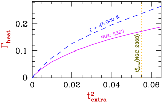
Figure 1: $\Gamma_{\rm heat}$ as a function of $t^{2}_{\rm extra}$ for the model of NGC 2363 (solid line) and for a simpler model (dashed line, see text). The $t^{2}_{\rm extra}$ value inferred from observations of NGC 2363 is also shown.

4 The kinetic luminosity of the stellar cluster

In this section, we will compare the kinetic luminosity of NGC 2363 to the heating rate implied by the observed temperature fluctuations. To estimate the kinetic luminosity produced by the stellar winds in NGC 2363, we considered a synthetic stellar population with the parameters resumed in Table 1. The only difference with respect to the model by Luridiana et al. (1999) is the adoption of $Z=0.004$ instead of $Z=0.005$, to avoid interpolation between spectra, and to allow a more direct comparison with the models by Binette & Luridiana (2000). This choice has little influence on the temperature-fluctuation problem, since we estimate that adopting $Z=0.005$ would increase the kinetic luminosity by less than 50% (Leitherer et al. 1992), which is not sufficient to change, as we will see, the results of this work.

Parameter	Value
SFR	Extended burst, $\Delta t=1.4$
$1+x$	2.00
$M_{\rm up}/M_{\odot}$	120
Age (Myr)	3.0
$Z$	0.004
$M_{\rm tot}(1\,\rm{M}_{\odot}\rightarrow 120\,\rm{M}_{\odot})$	$1.07\times 10^{5}\;\rm{M}_{\odot}$

Table 1: Adopted parameters for the stellar population in NGC 2363.

Three different estimates of the kinetic luminosity $L_{\rm kin}$ and the total integrated wind energy for this source are listed in Table 2. One of them was obtained with the first release of Starburst99 (see Leitherer et al. 1999) run with a theoretical wind treatment, which is the default set by the code and the one preferred by the authors of Starburst99. The other two were obtained with an updated version of the synthesis code of Cerviño & Mas-Hesse (1994) (hereafter CMHK, see Cerviño et al. (2001a) for details), with the wind treatment illustrated in Cerviño et al. (2001a). The reasons for considering two different synthesis codes with two different mass-loss laws reside in the importance of showing the effects of different assumptions on the wind treatment (a possibility granted by the Starburst99 code, which can be set to any of four different laws), together with the importance of estimating the expected statistical dispersion in the energy-related quantitities (a possibility granted by the CMHK code, either analytically or by means of Monte Carlo simulations). Stated otherwise, it is not our intention to compare the two codes, but rather the two wind treatments: had we chosen the same one as Cerviño et al. (2001a) in the Starburst99 settings, we would have found the same result as with the CMHK code.

The two estimates of $L_{\rm kin}$ obtained with the CMHK code have been obtained with an analytical and a Monte Carlo representation of the IMF respectively, and they both take into account the effect of statistical fluctuations in the IMF. When statistical effects in the IMF are taken into account, the population properties are no more univocally determined, being instead distributed along a probability distribution curve. The characteristic parameters of the curve can be determined analytically or by means of Monte Carlo simulations (see Cerviño et al. 2001b). The second line of Table 2 lists the analytical estimate of the average wind luminosity and the total integrated wind energy obtained with the CMHK code, as well as the corresponding 90% confidence intervals (i.e., the $5^{\rm th}$ and the $95^{\rm th}$ percentile). The third line quotes the same quantitites obtained by means of Monte Carlo simulations, again with the uncertainties corresponding to the 90% confidence interval. These two estimates of $L_{\rm kin}$ are in excellent agreement, showing the consistency of the two statistical approaches of the CMHK code. In all the cases, the extended burst scenario has been represented as the sum of individual instantaneous bursts of different ages and roughly equal masses. In the case of the Monte Carlo method, different simulations, taken from an ensemble of 5000 runs of $10^{2}$ stars each, have been summed up until the mass of each individual cluster was reached. The total number of independent Monte Carlo simulations of the extended burst obtained through this procedure was 64.

The average estimates obtained with CMHK give roughly 70% higher luminosity than the Starburst99 value; this is mainly due to the difference between the wind treatment adopted in the two codes, and is not directly related to differences in the spectra, which are, for the scopes of the present work, largely negligible. The integrated energy value obtained with Starburst99 is higher than the CMHK one, a somewhat surprising trend given the corresponding luminosity values. These figures depend on the winds evolution with time: the wind treatment adopted in the Starburst99 calculation gives less energetic winds than the one implemented in the CMHK code at earlier ages, while for ages greater than about 2.5 Myr the relationship is inverted.

Synthesis code	IMF filling	$L_{\rm kin}$	$E_{\rm kin}$
		($10^{39}$ erg s-1)	($10^{52}$ erg)
Starburst99	Analytical	$0.68$	5.0
CMHK	Analytical	${1.14}_{-0.23}^{+0.27}$	$4.34_{-0.61}^{+0.68}$
CMHK	Monte Carlo	${1.16}_{-0.20}^{+0.37}$	$4.32_{-0.66}^{+0.88}$

Table 2: Kinetic luminosities and integrated kinetic energies for the three considered SEDs.

It is now possible to compute the $\Gamma_{\rm heat}$ values associated with the kinetic energy input, according to the general expression:

$$\Gamma^{\rm kin}_{\rm heat}=\frac{L_{\rm kin}}{L_{\rm eq}+Q_{\rm eq}},$$ (6)

For simplicity, only one value for the equilibrium cooling rate will be used in the $\Gamma^{\rm kin}_{\rm heat}$ computations, resulting from a Cloudy model (Ferland 1996) of the region run with the Starburst99 SED:

$$L_{\rm eq}+Q_{\rm eq}=G_{\rm eq}^{\rm cooling}=1.46\times 10^{41}{\rm erg}\;{\rm s}^{-1},$$ (7)

and only the amount of kinetic luminosity deposited according to each SED will be varied. This introduces only a minor approximation, since the differences between synthesis codes, as well as the stochasticity of the IMF, affect the shape of the spectrum only marginally before the WR phase, which, in our extended-burst model accounts only for a minor fraction of the flux. This statement is not valid in general, since for WR-dominated bursts, a large dispersion is expected in the ionizing flux, hence in the cooling rate: see Cerviño et al. (2001b).

The $\Gamma^{\rm kin}_{\rm heat}$ values obtained are listed in Table 3, together with the inferred $t^{2}_{\rm extra}$ obtained from the hot-spot model of NGC 2363 (cf. Figure 1); we will refer to these $t^{2}_{\rm extra}$ values with the symbol $t^{2}_{\rm kin}$ to emphasize that they are inferred under the assumption that the temperature fluctuations are driven by the stellar-wind kinetic energy. All the $t^{2}_{\rm kin}$ values obtained are extremely small, well below the $t^{2}_{\rm extra}$ inferred from observations. However, there are still a few issues to consider before drawing any conclusion from the comparison between the $t^{2}_{\rm kin}$ values of Table 3 and the $t^{2}_{\rm extra}$ value of NGC 2363 inferred in Sect. 3.1.

Synthesis code	IMF filling	$\Gamma^{\rm kin}_{\rm heat}$	$t^{2}_{\rm kin}\times 10^{3}$
Starburst99	Analytical	0.0047	0.60
CMHK	Analytical	${0.0076}_{-0.0015}^{+0.0021}$	$0.96_{-0.19}^{+0.30}$
CMHK	Monte Carlo	${0.0076}_{-0.0011}^{+0.0028}$	$0.96_{-0.14}^{+0.40}$

Table 3: $\Gamma^{\rm kin}_{\rm heat}$ values associated to the wind luminosities, and inferred $t^{2}_{\rm kin}$ values.

5 Discussion

5.1 Wind-luminosity thermalization

An important issue to consider is the thermalization efficiency of the wind kinetic energy. Even assuming that our estimates of the wind luminosities in NGC 2363 are highly accurate, the derived $t^{2}_{\rm kin}$ values should be corrected downward to take into account the fraction of the energy injected to the ISM which is eventually thermalized.

1-D hydrodynamical models of the bubble around OB associations indicate that such fraction is about 80% (Plüschke 2001; Plüschke et al., in preparation). An estimate of the thermalization efficiency in the case of NGC 2363 can be made by comparing the total kinetic energy injected into the region since the beginning of the starburst to the observed kinetic energy. Roy et al. (1991) observed in NGC 2363 a bubble with a 200 pc diameter, expanding with a velocity of 45 km s^-1, and calculated that the total kinetic energy involved is $E_{\rm kin}^{\rm obs}\sim 2\times 10^{52}$ ergs, in agreement with the estimate made by Luridiana et al. (1999). Roy et al. (1992) found a high-velocity component in the gas, with a kinetic energy of $E_{\rm kin}^{\rm obs}\sim 10^{53}$ ergs. González-Delgado et al. (1994) confirmed the presence of this high-velocity gas, and estimated a kinetic energy of $E_{\rm kin}^{\rm obs}\sim 3\times 10^{52}$ ergs.

These figures should be compared to the estimated values of the integrated wind kinetic energy, which are listed in Table 2 for the three considered cases. If we add the kinetic energy of the low-velocity bubble observed by Roy et al. (1991) to that of the high-velocity gas observed by González-Delgado et al. (1994), we find that the efficiency of the thermalization of wind kinetic energy is close to 0, lowering further the computed $t^{2}_{\rm kin}$ values.

An independent estimate of the efficiency of the thermalization of the wind energy can be done by considering the X-ray component in the spectrum of NGC 2363 detected by Stevens & Strickland (1998) with ROSAT; they found $L_{x}\mathrel{\hbox{\hbox to0.0pt{\hbox{\lower 4.0pt\hbox{$\sim$}}\hss}\hbox{$>$}}}6.6\times 10^{37}$ erg s^-1 assuming a distance of 3.44 Mpc to the object, which becomes $L_{x}\mathrel{\hbox{\hbox to0.0pt{\hbox{\lower 4.0pt\hbox{$\sim$}}\hss}\hbox{$>$}}}7.3\times 10^{37}$ erg s^-1 rescaling to the distance of 3.8 Mpc assumed by Luridiana et al. (1999). Assuming that the origin of the X-ray component is the reprocessing of the wind kinetic energy, we can infer typical values for the thermalization efficiency of the order $\mathrel{\hbox{\hbox to0.0pt{\hbox{\lower 4.0pt\hbox{$\sim$}}\hss}\hbox{$>$}}}$ 10%.

5.2 Pure photoionization component

The value of $t^{2}_{\rm str}$ could be higher if the ionizing spectrum turned out to be harder than supposed, as implied by the X-ray component detected by Stevens & Strickland (1998); in this case, the need for an extra-heating source to be added to the photoionization model would be proportionally smaller. To investigate this possibility, we computed a Cloudy model with the analytical SED of the CMHK code, modified to account for the transformation of 20% of the kinetic energy into X rays (Cerviño et al., in preparation). This experimental model is energetically equivalent to a hot-spot model in which the extra heating is provided by the wind kinetic luminosity thermalized with a 20% efficiency. Indeed, we found that for this model $t^{2}_{\rm str}=0.009$, i.e. the same as the Luridiana et al. (1999) to within 0.001, confirming that the wind kinetic luminosity is energetically insufficient to account for the observed temperature fluctuations.

5.3 Influence of stellar rotation

As it has been pointed out by Meynet & Maeder (2000), rotation dramatically changes the properties of massive-star models. In particular, it increases the mechanical energy released to the ISM (see, e.g., Maeder & Meynet 2001). Additionally, the winds of rotating massive stars can be highly non-spherical, with strong polar or equatorial structures, depending on the effective temperature and angular velocity of the star (Maeder & Desjacques 2001).

Rotation makes it possible to explain in several cases the observed features of individual stars, but, unfortunately, the evaluation of its effects on the integrated spectrum of star forming regions is not feasible yet. First, the distribution of angular velocities of the stars in the cluster should be known. Second, the distribution of inclination angles should also be known, since the emitted luminosity depends on the inclination angle. Third, it would be necessary to establish new homology relations in order to obtain the isochrones needed to compute the emission spectrum at any given time.

Thus, we can only predict qualitatively that rotating stars certainly produce a turbulent interstellar medium, possibly with strong density and temperature inhomogeneities, due to both the increased wind energy and the anisotropy of their winds. From the point of view of our study, the increased energy injected into the medium, would translate into a correspondingly higher $\Gamma^{\rm kin}_{\rm heat}$ value, and the turbulence created in the ISM would possibly increase the thermalization efficiency of such energy, in such a way that the ‘actual’ $\Gamma_{\rm heat}$ of the region would approach its upper limit $\Gamma^{\rm kin}_{\rm heat}$ (see also Sect. 5.1).

Thus, at a qualitative level, the effect of stellar tracks with rotation on our temperature-fluctuation model would be to increase the temperature fluctuation amplitude theoretically achievable through energy injection by stellar winds, as compared to non-rotating models.

5.4 Distance to NGC 2366

The distance to NGC 2366 plays several roles in our analysis. First, the average properties of a photoionization model constrained by observational data depend on the assumed distance in complex ways. Second, a smaller distance implies a smaller region, hence a relatively larger statistical dispersion. Third, the hot-spot model is calibrated to a specific model, so that, should the photoionization model change, the hot-spot model would also change.

In our analysis, based on the photoionization model by Luridiana et al. (1999), we assumed for the distance the value 3.8 Mpc determined by Sandage & Tammann (1976). However, there are a number of more recent distance determinations indicating smaller distances: Tikhonov et al. (1991) derived a distance of 3.4 Mpc to NGC 2366 through photographic photometry of its brightest stars; Aparicio et al. (1995) obtained the value of 2.9 Mpc with CCD photometry of its brightest stars; Tolstoy et al. (1995) determined a distance of 3.44 Mpc from Cepheid light curves and colors; Jurcevic (1998) obtained the value 3.73 Mpc, with an associated error of 0.04 dex, from a study of the period-luminosity relationship of the red supergiant variables in NGC 2366.

To illustrate how our conclusions would change under a different assumption on the distance, we consider a value of 3.4 Mpc, i.e. $\sim$10% less than the assumed distance. Given the observed H$\beta$ intensity, the smaller distance yields a 20% smaller rate of ionizing photons, Q(H⁰). Since in this case the region turns out to be smaller both in linear and in angular dimensions, more input parameters should be changed, in order to fulfill the observational constraint on the observed size of the nebula, even if the remaining constraints, such as the relevant line ratios, change negligibly. Though it is beyond the scope of this paper to calculate a full revised photoionization model, we can expect that a satisfactory fit could be obtained by means of relatively small adjustments in the density structure of the nebula surrounding the ionizing cluster, with the model stellar population rescaled to a total mass $M^{\prime}_{\rm tot}=0.80\times M_{\rm tot}$, and the other stellar parameters (e.g., SFR, IMF, etc.) left unchanged. These changes would translate into a $\Gamma^{\rm kin}_{\rm heat}$ smaller by 20%, with a statistical dispersion proportionally larger, due to the larger relative weight of the statistical fluctuations in the cluster.

The hot-spot model should also be accordingly modified, to take into account the properties of the revised model. However, we don’t expect it too change too much, since the ionization parameter of the revised model would be essentially the same as the one of the old model. Summarizing, we estimate that a downward revision of the assumed distance would not significantly change our conclusions.

5.5 Temperature-fluctuation profile

In the interpretation of our results, it is important to take into account that they were obtained for a rather specific temperature-fluctuation pattern. As stated by Binette & Luridiana (2000), the model returns the correct results for fluctuations resembling those depicted in their Figure 1, but for radically different patterns of hot spots (different in frequency, width, and/or amplitudes) the model would only provide a first order estimate of the relationship between $t^{2}$ and $\Gamma_{\rm heat}$; Binette & Luridiana (2000) estimate that the total uncertainty on $\Gamma_{\rm heat}$ resulting from this approximation is less than 20%.

6 Conclusions

Our results suggest that the kinetic energy provided to the ISM by the stars through stellar winds cannot account for the observed temperature fluctuations in NGC 2363. This result holds even if a thermalization efficiency of 100% is assumed; however, the comparison of the observed kinetic energy with the theoretical estimate of the wind kinetic energy suggest that such efficiency is rather low. These results confirm the conclusion drawn by Binette et al. (2001), and leave the question of the nature of energy source of temperature fluctuations open. New insights into the problem could possibly come from the use of stellar tracks with rotation, and/or the consideration of a temperature-fluctuation pattern radically different from the one used in the present work.