Nonlinear Beat Cepheid and RR Lyrae Models

The numerical hydrodynamic modelling of beat Cepheid behavior has been a long standing quest in which purely radiative models had failed consistently. We find that beat pulsations occur naturally when turbulent convection is accounted for in our hydrodynamics code. The development of a relaxation code and of a Floquet stability analysis greatly facilitates the search for and the analysis of beat Cepheid models. The conditions for the occurrence of beat behavior can be understood easily and at a fundamental level with the help of amplitude equations.

1 Introduction

Double-mode or beat pulsations are not uncommon among RR Lyrae (the RRd stars) and classical Cepheids (cf.  e.g. Kovács 2001). Yet the numerical modelling of this phenomenon remained an unmet challenge for years. Partial success was achieved with purely radiative codes (Kovács & Buchler 1993), but it took the incorporation of a model for turbulent convection into the hydrocodes to obtain results that are both robust and have astrophysical parameters that are in agreement with the observations. Essentially simultaneously, but independently, Kolláth et al. (1998) could model double-mode pulsations in Cepheid models and Feuchtinger (1998) in RR Lyrae models. In this paper we present an extension of this earlier work. We examine in some detail specific examples of both RR Lyrae and Cepheid models, as well as sequences of such models (in which L and M are held fixed and $T_{\rm{ef\!f}}$ is varied, thus mimicking approximately the horizontal branch and the Cepheid loops, respectively).

2 Turbulent Convection Model Equations

The turbulent convection model equations that we have incorporated in our hydrodynamics code are essentially those of Gehmeyr & Winkler (1992) and Kuhfuß (1986). They differ in the expression for the convective flux $F_{c}$ from those of Stellingwerf (1982) and Bono & Stellingwerf (1994) and those of original paper (Yecko, Kolláth & Buchler 1998), but are essentially the same as used by Wuchterl & Feuchtinger (1998). To be specific we reproduce here the equations that we use in our hydrodynamics code.

The fluid dynamics part of the model calculations are given by the following equations:

$${du\over dt} = -{1\over\rho}{\partial\over\partial r}\left(p+\thinspace\thinspace p_{t}+p_{\nu}\thinspace\thinspace\right)-{GM_{r}\over r^{2}}\quad\quad$$ (1)

$$\ \ \ \ {d\thinspace e\over dt}+p\thinspace{d\thinspace v\over dt} = -{1\over\rho r^{2}}{\partial\over\partial r}\left[r^{2}\left(F_{r}+\thinspace\thinspace F_{c}\thinspace\thinspace\right)\right]-\thinspace\mathbf{{\cal C}}\quad\quad$$ (2)

The turbulent motion of the gas and the convection interacts with the hydrodynamics of the radial motion through the convective flux $F_{c}$, the viscous eddy pressure $p_{\nu}$ the turbulent pressure $p_{t}$, and finally, through an energy coupling term ${\cal C}$. The turbulent energy $e_{t}$ is determined by a time dependent diffusion equation

$${de_{t}\over dt}+\left(p_{t}+p_{\nu}\right)\thinspace{d\thinspace v\over dt}=-{1\over\rho r^{2}}{\partial\over\partial r}\left(r^{2}F_{t}\right)+{\cal C}\quad\quad\\$$

The coupling term that connects the gas and the turbulent energy equations is given by:

$${\cal C}=\alpha_{d}\thinspace{e^{\scriptscriptstyle 1/2}_{t}\over\Lambda}\left(S_{t}-e_{t}\right),$$ (3)

where $\Lambda=\alpha_{\Lambda}\thinspace H_{p}$, $H_{p}=p\thinspace r^{\scriptstyle 2}/(\rho GM)$ is the pressure scale height, $\alpha_{\Lambda}$ is the mixing length parameter. The $\alpha_{d}$’s are dimensionless parameters of order unity. Both the convective flux and the source term of the turbulent energy ($S_{t}$) depend on the dimensionless entropy gradient

$$Y = -{H_{p}/c_{p}}\thinspace\thinspace{\partial s/\partial r}$$ (4)

$$S_{t} = (\alpha_{s}\thinspace\alpha_{\Lambda})^{\scriptstyle 2}{p\over\rho}\thinspace\beta T\thinspace\thinspace Y\,f_{pec}$$ (5)

The remaining quantities are defined as

$$p_{t} = \alpha_{p}\thinspace\rho\thinspace e_{t},$$ (6)

$$p_{\nu} = -\frac{4}{3}\alpha_{\nu}\thinspace\rho\Lambda e^{\scriptscriptstyle 1/2}_{t}r{\partial\thinspace\over\partial r}{u\over r}$$ (7)

$$F_{t} = -\alpha_{t}\thinspace\rho\Lambda e^{\scriptscriptstyle 1/2}_{t}{\partial\thinspace\thinspace e_{t}\over\partial r}$$ (8)

$$F_{c} = \alpha_{c}\alpha_{\Lambda}\thinspace\rho e_{t}^{{\scriptscriptstyle 1/2}}\thinspace c_{p}T\thinspace Y\,f_{pec}.$$ (9)

$$f_{pec}={1\over 1+\alpha_{r}Pe^{-1}},\quad\quad Pe =D_{c}/D_{r}$$ (10)

$$D_{r}={4\over 3}{acT^{3}\over\kappa\rho^{2}c_{p}},\quad\quad D_{c} =\Lambda e_{t}^{\scriptscriptstyle 1/2}$$ (11)

The turbulent convective equations can be derived on dimensional and physical grounds with a number of dimensionless parameters ($\alpha$’s) that are of order unity but for which theory provides no numerical values. Our approach has been to attempt to calibrate them through a comparison of our results with the observational data.

The calibration of the $\alpha$’s is a daunting task because of the large number of parameters on the one hand, and the large number of observational constraints, many of which require extensive full amplitude hydrodynamical model calculations. For example, important constraints are the locations and widths of the fundamental and first overtone instability strips, the Fourier decomposition coefficients of the light curve and of the radial velocity data, with their dependence on metallicity. Such a global calibration has not yet been performed, and it is not even sure that it possible given the rather simple turbulent convection recipe that we use. In that sense our results must be regarded as tentative. We stress however, that the types of behavior that we describe here are not sensitive to these $\alpha$’s, but that the masses, luminosities and $T_{\rm{ef\!f}}$’s at which they occur depend on them. In Kolláth & Buchler (2001) we have presented typical modal selection diagrams for Cepheid and RR Lyrae models (figures 14 and 15) that show the calculated pulsational behavior of the models in a Hertzsprung-Russell diagram.

3 Transient Behavior of Models

The first issue that we address concerns the confirmation that a given model is indeed undergoing stable double-mode pulsations rather than being involved in a switch from one mode to another. Deciding on the basis of a single hydrodynamical calculation whether a model is undergoing steady double-mode pulsations can be fraught with peril. The model may give the false impression of having achieved steady behavior when it is actually still in a transient state even after thousands of periods of integration, and it will end up pulsating with a single frequency. The reason for this will become clear shortly.

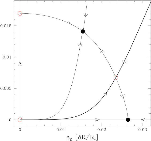
Figure 1: Cepheid model with $T_{\rm{ef\!f}}$=5580 K. Left: The flow in the ($A_{0},A_{1}$) phase space. The large dots represent the hydrodynamical results at equal time intervals, so that the spacing of the dots gives an indication of the speed. The short lines represents the flow field (dots denote the base of the normalized vectors). Right: The stable/unstable fixed points are denoted by filled/open circles. The integral lines (heteroclinic connections) that connect the fixed points are shown as solid lines with arrows indicating the evolution direction. The thick line is also the separatrix, i.e. the boundary between the basins of attraction of the two stable fixed points, viz.the stable DM and the fundamental.

3.1 Time Dependence of Amplitudes and Phases

One of the several tools that are needed is the calculation of the time dependence of the amplitudes and phases of the modes that are excited in the models. Instead of using a time dependent Fourier analysis as advocated by Kovács, Buchler & Davis (1987, KBD87) we now use the much more powerful and accurate analytical signal method of Gábor (1946) to reconstruct the time dependent amplitudes and frequencies of the pulsation modes. (cf.  e.g.,  Cohen 1994). The method can be extended to multi-component signals with the help of filters that restrict the power to the desired frequency components. It is convenient to make this filtering in Fourier space where it involves just a product, and to combine it with the definition of the analytical signal (Kolláth & Buchler 2001)

$$\negthinspace\negthinspace Z_{k}(t) = a_{k}(t)e^{i\varphi_{k}(t)}$$ (12)

$$= \frac{1}{\pi}\int^{\infty}_{0}d\omega H(\omega-\omega_{k})e^{i\omega t}\int_{-\infty}^{\infty}dt^{\prime}s(t^{\prime})e^{-i\omega t^{\prime}},$$

where $s(t)$ is the real valued signal that is to be analyzed, $H(\omega-\omega_{k})$ is the filtering window that is centered on the desired $\omega_{k}$. A Gaussian window with a half width of $\omega_{k}/10$ generally gives satisfactory results for the stellar pulsations. The resulting amplitudes and phases describe then the transient behavior of the given mode. The analytical signal approach yields a much better resolution than the KBD87 approach because it is not necessary to average the amplitudes in time to get smooth results.

With the analytical signal method it is therefore very easy and fast to define unambiguously the instantaneous phase $\varphi(t)$ and amplitude $A(t)$ of a signal.

3.2 Phase Plots

The computed time dependent amplitudes, in our case $A_{0}(t)$ and $A_{1}(t)$, can then be used to visualize the transient behavior of the pulsating model in an ($A_{0}$,$A_{1}$) phase space. Our amplitudes are defined as those of the normalized radial displacement of the photosphere, $\delta R_{ph}/R_{*}$, where $R_{*}$ is the photospheric radius of the equilibrium model.

In Fig. 1 on the left we display the results of a number of hydrodynamical calculations made for the same Galactic Cepheid model (M=4.7 $M_{\sun}$, L=1335 $L_{\sun}$, $T_{\rm{ef\!f}}$ = 5580 K, Z=0.02), but started (kicked from the unstable equilibrium) with different initial conditions. The tracks all start with small amplitudes (lower left side).

Several notable features stand out in the left of Fig. 1. Since the thick dots denote points that are equally separated in time one sees that the models all evolve very quickly toward an arc along which the transient evolution is extremely slow. If only one model were computed this ’convergence’ could easily be misinterpreted as a steady double-mode pulsation. The figure indicates that the point on the $A_{0}$ axis with ($A_{0}=0.026,A_{1}=0$) is an attractor. The three rightmost tracks transit to this fundamental attractor after a sufficiently long integration time. This corresponds of course to the fundamental limit cycle. Similarly the point on the arc with ($A_{0}=0.023,A_{1}=0.007$) repels the tracks, and it corresponds to an unstable double-mode pulsation. Further up along the arc a second attractor with ($A_{0}=0.015,A_{1}=0.014$) is clearly visible. Six of the tracks converge toward it from the left and three of them from the right. This attractor corresponds to stable double-mode pulsations. Finally, one notes that the single-mode overtone limit cycle at ($A_{0}=0,A_{1}=0.017$) repels because it is unstable. All tracks run away from the origin because the equilibrium model is linearly unstable in both modes.

We shall see that this whole picture can be clearly understood after we have introduced amplitude equations. They allow us to draw the flowfield that has been superposed on the left-hand figure.

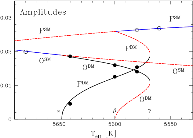
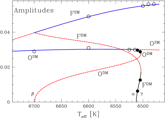
Figure 2: Left: Behavior of the amplitudes of single-mode (SM) and double-mode (DM) pulsations along a constant $L$ convective Cepheid model sequence; Solid lines: stable pulsations, dashed lines: unstable pulsations; cf.  text. The filled and open circles locate calculated hydro-models. Right: RR Lyrae sequence. (Amplitude in units of $\delta R_{ph}/R_{*}$.)

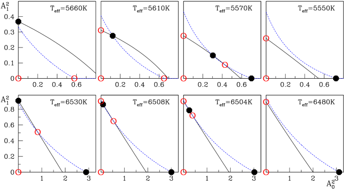
Figure 3: Switch from single-mode overtone to double-mode pulsation for a Cepheid (top) and a RR Lyrae (bottom) model sequence; Solid circles: stable fixed points, open circles: unstable fixed points. ($A^{2}$ in units of $10^{-3}(\delta R_{ph}/R_{*})^{2}$.)

3.3 Amplitude Equations

It has been known for a while now that one can develop a global understanding of the ’modal selection’ problem with the help of the amplitude equation formalism (Buchler & Goupil 1984). The beauty and power of the amplitude equations are their simplicity and their very basic and generic nature. They apply to any system, be it a pulsating star, a biological system, or any other dynamical system, in which (a) the relative growth-rates of the excited modes are small; (b) the pulsations are sufficiently weakly nonlinear so that an expansion in the amplitudes is justified. Only selected powers of the amplitudes appear (Buchler & Goupil 1984, Buchler 1993), and the omitted terms are unessential for the modal selection (bifurcation diagram), i.e.,  the nature of the dynamical behavior does not depend on them.

Condition (a) is clearly satisfied for RR Lyrae and classical Cepheids, since typically the growth-rates are of the order of a percent of the frequencies. That condition (b) is also satisfied manifests itself, for example, by the fact that the nonlinear periods are very close to the linear ones.

The form that the amplitude equations take on depends on whether or not there are nearby resonances. For the beat RR Lyrae there is no low-order resonance in the period range of interest, and for the beat Cepheids the nearest resonance is too far to be influential. The appropriate amplitude equations for the nonresonant case are

$$\dot{a}_{0} \negthinspace\negthinspace\negthinspace=\negthinspace\negthinspace\negthinspace a_{0}\thinspace(\sigma_{0}+Q_{00}|a_{0}|^{2}+Q_{01}|a_{1}|^{2}+S_{0}|a_{0}|^{2}|a_{1}|^{2}$$ (13)

$$\leavevmode\nobreak\ \leavevmode\nobreak\ +R_{00}|a_{0}|^{4}+R_{01}|a_{1}|^{4})$$

$$\dot{a}_{1} \negthinspace\negthinspace\negthinspace=\negthinspace\negthinspace\negthinspace a_{1}\thinspace(\sigma_{1}+Q_{10}|a_{0}|^{2}+Q_{11}|a_{1}|^{2}+S_{1}|a_{0}|^{2}|a_{1}|^{2}$$ (14)

$$\leavevmode\nobreak\ \leavevmode\nobreak\ +R_{10}|a_{0}|^{4}+R_{11}|a_{1}|^{4})$$

where the dot represents the time-derivative and $\sigma_{j}$ are the linear eigenvalues for an assumed $\exp(\sigma t)$ dependence,

$$\sigma_{j}=\kappa_{j}+i\omega_{j}$$ (15)

The $a_{j}$’s are the complex amplitudes of the two excited modes, and $Q_{jk}$, $S_{j}$ and $R_{jk}$ are the complex nonlinear coupling constants.

It is found to be more convenient to use real amplitudes $A_{j}(t)$ and phases $\varphi_{j}(t)$, defined by $a_{j}(t)=A_{j}(t)\exp i\varphi_{j}(t)$, because this produces a complete decoupling of the amplitudes from the phases. One finds

$$\dot{A}_{j} = A_{j}\thinspace\thinspace\thinspace(\kappa_{j}+q_{j0}A_{0}^{2}+q_{j1}A_{1}^{2}$$ (16)

$$\quad\quad\quad\quad+s_{j}A_{0}^{2}A_{1}^{2}+r_{j0}A_{0}^{4}+r_{j1}A_{1}^{4})$$

and

$$\dot{\varphi}_{0} = \omega_{0}+\hat{q}_{00}A_{0}^{2}+\hat{q}_{01}A_{1}^{2}+\hat{s}_{0}A_{0}^{2}A_{1}^{2}$$ (17)

$$\dot{\varphi}_{1} = \omega_{1}+\hat{q}_{10}A_{0}^{2}+\hat{q}_{11}A_{1}^{2}+\hat{s}_{1}A_{0}^{2}A_{1}^{2}$$ (18)

where

$$Q_{jk} = q_{jk}+i\thinspace\hat{q}_{jk}$$ (19)

$$S_{j} = s_{j}\thinspace\thinspace+i\thinspace\hat{s}_{j}$$ (20)

$$R_{jk} = r_{jk}+i\thinspace\hat{r}_{jk}.$$ (21)

We have disregarded the imaginary parts of the higher order terms in the phases because they are unimportant. One also notes that all equations can be expressed in terms of the squares $A_{0}^{2}$ and $A_{1}^{2}$.

The constant amplitude solutions of Eqs. (13, 14) the so-called fixed points are therefore obtained from solving the equations

$$\kappa_{0} + q_{00}A_{0}^{2}+q_{01}A_{1}^{2}+s_{0}A_{0}^{2}A_{1}^{2}$$ (22)

$$\quad\quad\quad\quad+r_{00}A_{0}^{4}+r_{01}A_{1}^{4}=0$$

$$A_{1} = 0$$ (23)

$$\kappa_{1} + q_{10}A_{0}^{2}+q_{11}A_{1}^{2}+s_{1}A_{0}^{2}A_{1}^{2}$$ (24)

$$\quad\quad\quad\quad+r_{10}A_{0}^{4}+s_{11}A_{1}^{4}=0$$

$$A_{0} = 0$$ (25)

pairwise between the two sets. They correspond to steady nonlinear pulsations. In the earliest use of amplitude equations for describing DM pulsations (Buchler & Kovács 1986; Kolláth et al. 1998) the amplitude equations were truncated at the lowest nontrivial, i.e. the cubic terms. It was shown that in this order the single-mode fixed points and steady DM pulsations cannot simultaneously be stable for the same stellar model. Since then it has been realized that the behavior of the hydrodynamical models and the observational constraints imposed by the Beat Cepheids and RR Lyrae stars can be a little more complicated than the cubic nonresonant amplitude equations allow. However, the more complicated behavior can be captured if we keep the next order nontrivial terms, viz. the quintic ones in the amplitudes (Buchler et al. 1999). It is not necessary though to keep all quintic terms, and for simplicity, these authors retained only the $r_{00}$ and $r_{11}$ cubic terms and discussed the fixed points of the amplitude equations. Here we keep instead the $s_{0}$ and $s_{1}$ cubic terms because they give a slightly better description of the results of the hydrodynamical calculations.

3.4 Determination of the Nonlinear Coefficients

We can use the hydrodynamical calculations that are reported in Fig. 1 to determine the values of the unknown nonlinear coupling coefficients that appear in the amplitude equations. This is done as follows: The analytical signal method gives the time dependent amplitudes sufficiently accurately so that the derivatives $\dot{A}$ can be used directly in Eqs. 16 to obtain the linear growth rates and the nonlinear coupling coefficients in these equations through a linear least squares fit. (With the method described in Buchler & Kovács (1987) it was necessary to make a tedious nonlinear fit.)

Once the coefficients are known, we can then produce a vector plot ${\bf u}=(\dot{A}_{0},\dot{A}_{1})$. The computed vector plot has been superposed on the transient evolutionary tracks in Fig. 1, and gives a global view of the flow field. (The dots represent the bases of the vectors). The speeds have been normalized because they span a very broad range of values.

The fixed point scenario is summarized in the right side of Fig. 1. The solid circles denote the stable fixed points and the open circles the unstable ones. We recall that the five fixed points each correspond to a steady pulsational behavior. The origin represents the unstable equilibrium model (an unstable node point; for a mathematical definition of these terms cf. Lefshetz 1977), the two fixed points on the axes are the stable fundamental and unstable first overtone limit cycles (a stable node point and a saddle node point, respectively). The remaining two fixed points are the stable and unstable double-mode pulsations (again a stable node point and a saddle node point, respectively). Also shown in the figure are the integral lines that link the fixed points (the heteroclinic connections), and the special one, the separatrix (thick line), that separates the two attractor, i.e. the regions of initial conditions that lead to the stable DM pulsation and to the fundamental limit cycle, respectively.

The amplitude equations give an accurate and global picture of the pulsational behavior of the models.

TABLE 1.- Nonlinear Coupling Coefficients and Growth Rates.
$T_{ef\!f}[K]$	$q_{00}$ [$d^{-1}$]	$q_{01}$ [$d^{-1}$]	$q_{10}$ [$d^{-1}$]	$q_{11}$ [$d^{-1}$]	$s_{0}$ [$d^{-1}$]	$s_{1}$ [$d^{-1}$]	$\kappa_{0}$ [$d^{-1}$]	$\kappa_{1}$ [$d^{-1}$]
Convective Cepheid Model sequence.
5560	–0.92	–1.49	–5.77	–11.99	–3436.0	2449.0	0.00066	0.00329
5580	–0.93	–1.50	–5.62	–12.17	–2816.0	4994.0	0.00065	0.00351
5600	–0.94	–1.45	–5.48	–12.03	–2653.0	6594.0	0.00063	0.00370
5640	–0.98	–1.63	–5.14	–11.53	–2054.0	5567.0	0.00060	0.00408
5680	–1.03	–1.87	–4.66	–10.91	–1545.0	830.7	0.00057	0.00441
Convective RR Lyrae Model sequence.
6480	–3.08	–10.28	–19.81	–44.26	–2701.0	–1000.0	0.00964	0.03953
6500	–3.09	–10.18	–20.24	–43.98	–2826.0	–545.7	0.00936	0.03961
6505	–3.07	–10.13	–20.35	–43.94	–2750.0	–500.4	0.00924	0.03967
6515	–3.08	–10.08	–20.62	–43.90	–2833.0	–383.7	0.00910	0.03976
6525	–3.07	–9.99	–20.75	–43.72	–2792.0	–359.9	0.00890	0.03971
6600	–3.22	–9.92	–22.26	–42.38	–2781.0	36.2	0.00774	0.03866
6700	–3.85	–10.08	–22.29	–40.16	–2012.0	–3303.0	0.00605	0.03519

4 Sequences of Models

4.1 Turbulent convective models

In this section we examine constant $L$ and $M$ sequences of turbulent convective models, one for Cepheids and one for RR  Lyrae stars. These sequences display a somewhat different behavior, but that has more to do with the chosen stellar parameters L and M than with the nature of the stars. In fact both Cepheids and RR Lyrae exhibit both types of behavior in some range of L and M.

4.1.1 Cepheid Sequence:

In Fig. 2 we report the results of the convective Cepheid model sequence (M=4.7 $M_{\sun}$, L=1335 $L_{\sun}$) with $T_{\rm{ef\!f}}$ varying from 5690 to 5530 K. The solid circles correspond to the amplitudes of the computed stable DM pulsators, and the open circles to single-mode first overtone or fundamental pulsators.

In Table 1a we show the nonlinear coupling coefficients for the Cepheid sequence. The calculations are laborious albeit straightforward, because for each model in the sequence to the numerical hydrodynamics calculations have to be made for a set of different initial conditions, and then the coefficients have to be computed through a nonlinear fit. One notes that the coefficients do not vary much from one model to another. This, by the way, serves also as a confirmation of the quality of our fits.

The lines in Fig. 2 show the amplitudes of the possible pulsational states of the models. The lines were obtained by computing the fixed points of the amplitude equations with average values of the nonlinear coupling constants, but using the $T_{\rm{ef\!f}}$ dependent growth rates $\kappa_{0}$ and $\kappa_{1}$.

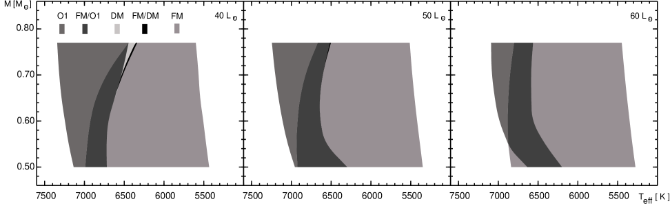
Figure 4: Modal selection of RR Lyrae model sequences The gray shading of the modal states are described at the top of the left figure: F: fundamental mode, F/DM either fundamental or double mode, DM double mode, F/O1 either fundamental or first overtone, O1 first overtone

The solid lines denote stable and the dashed lines unstable behavior. The first overtone limit cycle is seen to be stable down to $T_{\rm{ef\!f}}$ = 5647 K. The fundamental limit cycle is stable up to $T_{\rm{ef\!f}}$= 5598 K, and a stable DM pulsation exists between $T_{\rm{ef\!f}}$ = 5647 and 5568 K. (A second DM pulsation is also possible between $T_{\rm{ef\!f}}$ = 5598 and 5568 K, but is unstable and therefore astronomically not achievable.) The sequence thus shows hysteresis, i.e. in the range $T_{\rm{ef\!f}}$ = 5598 to 5568 K the pulsational state depends on whether the stellar evolution is blueward or redward.

Because Eqs. (22  – 25) are a function of the squared amplitudes, another visualization of the bifurcation scenario is afforded by Fig. 3 which shows the fixed points in an ($A_{0}^{2}$,$A_{1}^{2}$) plot for the same Cepheid model sequence. The loci defined by Eqs. (22, 24) are shown as dashed and solid lines, respectively. The remaining two loci are the positive x and y axes. The solid and open circles represent stable and unstable fixed points which are the intersections of these loci.

4.1.2 RR Lyrae Sequence:

The results of this sequence are reported in Fig. 2. Here we have the possibility of a fundamental limit-cycle with $T_{\rm{ef\!f}}$ $<$ 6700K, of an overtone limit-cycle with $T_{\rm{ef\!f}}>$ 6500 K. The $T_{\rm{ef\!f}}$ range of DM behavior is extremely narrow. Again we have hysteresis. Along a redward track the model starts off as an RRc star, then becomes a beat RR Lyrae (RRd) and finally changes into an RRab. Along a blueward excursion the model starts of a RRab and then turns into an RRc, without ever being RRd.

Compared to Fig. 2 the situation is now reversed in terms of the relative locations of points ${\bf\alpha}$ and ${\bf\gamma}$. Again, if we could disregard the quintic terms for the sake of argument, points ${\bf\alpha}$ and ${\bf\beta}$ would merge, and in the scenario described by Buchler & Kovács (1986), we are now in an ’either fundamental or overtone’ situation (${\cal D}<0$), as confirmed by the values in Table 1b for a sequence of RR Lyrae (M=0.77 $M_{\sun}$, L=50.0 $L_{\sun}$, Z=0.0001) models. The DM behavior occurs here only because of the looping back due to the quintic terms, and as a result is much narrower than in the Cepheid case.

Fig. 3 shows the fixed points in an ($A_{0}^{2}$,$A_{1}^{2}$) plot for the same RR Lyrae model sequence. The loci defined by Eqs. (22, 24) are shown as dashed and solid lines, respectively. The remaining two loci are the positive x and y axes. The solid and open circles represent stable and unstable fixed points which are the intersections of these loci.

We summarize the modal selection results obtained for a number of RR Lyrae sequences in Figure 4 which shows the regions in which the various pulsational behavior occurs. In these calculations the metallicity was at Z=0.0001, since according to our calculations the metallicity has only a minor effect of the RR Lyrae edges. All blue and red edges are nonlinear ones except for the F red edge, which is from linear stability analysis. Note that at low luminosity and high mass an additional F region appears. We caution again that these results depend on our choice of turbulent convective parameters and that they may have to be revised, at least quantitatively, when a more definitive calibration is performed.

5 Discussion

We have already pointed out that radiative models have failed to yield steady DM pulsations, at least with a behavior that satisfies the observations. It is therefore of interest to dwell a little on why convective models do.

First we note that the looping back between 5600 and 5570K in the Cepheid models and between 6510 and 6500K for RR Lyrae models in Fig. 2 occurs because of the presence of quintic terms in the amplitude equations. If for the sake of argument we were to ignore the quintic terms then the ${\bf\alpha}$ and ${\bf\gamma}$ points in Fig. 2 would merge, and would be to the right of the point ${\bf\alpha}$, where the fundamental amplitude vanishes.

In Figs. 3 the curves would turn into straight lines, as shown schematically in Fig. 5. In the situation depicted on the left side the model pulsates in either the F or the O1 limit cycle, depending on the past evolutionary history. The right side corresponds to the DM case. It is easily shown (Buchler & Kovács 1986) that a necessary condition for double-mode behavior is that ${\cal D}=q_{00}q_{11}-q_{01}q_{10}>0$. This condition is never found to be satisfied in purely radiative models in which the cross-coupling terms $q_{01}$ and $q_{10}$ always dominate over the self saturation terms $q_{00}$ and $q_{11}$.

One notes in Fig. 3 that the $T_{\rm ef\!f}$=5610K Cepheid model has the same topology as the right figure with the DM behavior, and that the $T_{\rm ef\!f}$=6530K RR Lyrae model has that of the left side. Table 1 shows that indeed ${\cal D}>0$ for the Cepheid model sequence and ${\cal D}<0$ for the RR Lyrae one, even though this criterion applies only approximately when the quintic terms are considered. Nevertheless it explains why the DM region in the convective Cepheid model sequence is much broader than that of the RR Lyrae (it would exist even in the absence of the quintic terms).

Figure 5: Schematic plot. Solid circles: stable fixed points, open circles: unstable fixed points. Left: F or O1 regime, ${\cal D}<0$ and Right: DM regime, ${\cal D}>0$.

In Kolláth et al. (1998) we had somewhat hastily suggested that the abrupt disappearance of the DM solution was probably due to a pole caused by the vanishing of ${\cal D}$. There is indeed a pole in the broad vicinity, but it is too far to play a role. Instead, as we have shown here, the behavior is due to the appearance and collision of two DM fixed points, a situation that is made possible because of the importance of the quintic terms which generate the two DM fixed points.

6 Conclusions

We have shown that there are two reasons for the occurrence of DM behavior with the turbulent convective models. One is the increase of the cubic saturation terms, $q_{00}$ and $q_{11}$, relative to the cross-coupling terms, $q_{01}$ and $q_{10}$. This is a rather subtle and hidden effect of turbulent dissipation because these coefficients are given as complicated integrals over the structure of the star (Buchler & Goupil 1984).

The other reason is the necessity to include quintic terms in the description which, in turn, enrich the complexity of the bifurcation diagram, in particular by causing the simultaneous occurrence of two DM fixed points – compare Figs. 3 and 5.

One of the interesting questions that we have not addressed concerns the time it takes to switch from one pulsational mode (fixed point) to another one. This problem, in our opinion, had never been correctly addressed in the pulsation literature, and we discuss it in a companion paper (Buchler & Kolláth 2001) where we show that this transition does generally not occur on the thermal time scale $t_{th}=\kappa^{-1}$, but on a much longer time scale, which, depending on the type of bifurcation is either set by the stellar evolution time scale, more precisely $(d\kappa/dt)^{-{\scriptscriptstyle 1/2}}$, or by the thermal time $t_{th}$, however generally multiplied by several orders of magnitude.

- (1) Bono, G.& Stellingwerf, R.F. 1994, ApJS, 93, 233
- (2) Buchler, J. R. 1993, in Nonlinear Phenomena in Stellar Variability, Eds. M. Takeuti & J.R. Buchler (Kluwer: Dordrecht), repr. from ApSS 210, 1.
- (3) Buchler, J.R. & Goupil, M.J. 1984, ApJ, 279, 394
- (4) Buchler, J.R. & Kolláth, Z. 2001, A&A to be submitted
- (5) Buchler, J.R. & Kovács, G. 1986, ApJ, 308, 661
- (6) Buchler, J.R. & Kovács, G. 1987, ApJ, 318, 232
- (7) Buchler, J. R., Yecko, P., Kolláth, Z. & Goupil, M. J. 1999, ASP Conference Series 183, 141
- (8) Cohen, L. 1994, Time-Frequency Analysis. Prentice-Hall PTR. Englewood Cliffs, NJ
- (9) Feuchtinger, M.U 1998, A&A, 337, 29
- (10) Gábor, D. 1946, Theory of communications, J.IEEE (London), 93, 429
- (11) Gehmeyr, M. & Winkler, K.H.A. 1992, A&A 253, 92; ibid. 253, 101
- (12) Kolláth, Z., Beaulieu, J.P., Buchler, J.R. & Yecko, P. 1998, ApJ Letters, 502, L55
- (13) Kolláth, Z. & Buchler, J. R. 2001, in Nonlinear Stellar Pulsation, Eds. M. Takeuti & D. Sasselov, Astrophys. & Space Sci. Library Vol. 257. p. 29., (astro-ph/0003386)
- (14) Kovács, G. 2001, in Nonlinear Stellar Pulsation, Eds. M. Takeuti & D. Sasselov, Astrophys. & Space Sci. Library Vol. 257. p. 61 (astro-ph/0003386)
- (15) Kovács, G. & Buchler, J.R. 1993, ApJ, 404, 765
- (16) Kovács, G., Buchler, J.R. & Davis, C.G. 1987, ApJ, 319, 247
- (17) Kuhfuss, R. 1986, A&A, 160, 116
- (18) Lefshetz, S. 1977, Differential Equations: Geometric Theory, (New York: Dover)
- (19) Stellingwerf, R.F. 1982, ApJ, 262, 330
- (20) Wuchterl, G. & Feuchtinger, M.U. 1998 A&A, 340, 419
- (21) Yecko, P., Kolláth Z. & Buchler, J.R. 1998, A&A, 336, 553