Clustering of Dark Matter Halos on the Light-cone

Yasushi Suto

Abstract

A phenomenological model for the clustering of dark matter halos on the light-cone is presented. In particular, an empirical prescription for the scale-, mass-, and time-dependence of halo biasing is described in detail. A comparison of the model predictions against the light-cone output from the Hubble Volume $N$ -body simulation indicates that the present model is fairly accurate for scale above $\sim 5h^{-1}$ Mpc. Then I argue that the practical limitation in applying this model comes from the fact that we have not yet fully understood what are clusters of galaxies, especially at high redshifts. This point of view may turn out to be too pessimistic after all, but should be kept in mind in attempting precision cosmology with clusters of galaxies.

Department of Physics and Research Center for the Early Universe, School of Science, University of Tokyo, Tokyo 113-0033, Japan.

1. Introduction

The standard picture of cosmological structure formation suggests that any visible object forms in a gravitational potential of dark matter halos. Therefore, a detailed description of dark halo clustering is the most basic step toward understanding the clustering of visible objects in the universe. For this purpose, many theoretical models for halo clustering have been developed and then tested against extensive numerical simulations.

First, I will describe our most recent theoretical model for clustering of dark matter halos (Hamana, Yoshida, Suto & Evrard 2001b). In particular, we focus on their high-redshift clustering where the past light-cone effect is important. Then I will show that our model predictions are in good agreement with the result from a light-cone output of the Hubble volume simulation (Evrard et al. 2001). Finally I will discuss a fundamental difficulty in relating the halo model to clusters of galaxies. My conclusion is that we already have a reliable empirical model for the halo clustering, but that we need to understand what are the clusters of galaxies, especially at high redshifts, before attempting precision cosmology with clusters of galaxies.

2. Theoretical model for two-point correlation functions of dark matter halo on the light-cone

As emphasized by Suto et al.(1999), for instance, observations of high-redshift objects are carried out only through the past light-cone defined at $z=0$ , and the corresponding theoretical modeling should properly take account of a variety of physical effects which are briefly summarized below.

2.1. Nonlinear gravitational evolution of dark matter density fluctuations

Assuming the cold dark matter (CDM) paradigm, the linear power spectrum of the mass density fluctuations is computed by solving the Boltzmann equation for systems of CDM, baryons, photons and (usually massless for simplicity) neutrinos. The resulting spectrum $P^{\rm R}_{\rm linear}(k,z)$ in real space is specified by a set of cosmological parameters including the density parameter $\Omega_{0}$ , the baryon density parameter $\Omega_{b}$ , and the Hubble constant $h$ in units of 100/km/s/Mpc, and the cosmological constant $\lambda_{0}$ . Then one can obtain its nonlinear counterpart in real space, $P^{\rm R}_{\rm nl}(k,z)$ by adopting a fitting formula of Peacock & Doods (1996).

2.2. Empirical model of halo biasing

The most important ingredient in describing the clustering of halos is their biasing properties. The mass-dependent halo bias model was developed by Mo & White (1996) on the basis of the extended Press-Schechter theory. Subsequently Jing (1998) and Sheth & Tormen (1999) improved their bias model so as to more accurately reproduce the mass-dependence of bias computed from $N$ -body simulation results. We construct an improved halo bias model of the two-point statistics which reproduces the scale-dependence of the Taruya & Suto (2000) bias correcting the mass-dependent but scale-independent bias of Sheth & Tormen (1999) on linear scales as follows:

	$\displaystyle b_{\rm halo}(M,R,z)$	$\displaystyle=$	$\displaystyle b_{\scriptscriptstyle\rm ST}(M,z)\left[1.0+b_{\scriptscriptstyle\rm ST}(M,z)\sigma_{M}(R,z)\right]^{0.15},$		(1)
	$\displaystyle b_{\scriptscriptstyle\rm ST}(M,z)$	$\displaystyle=$	$\displaystyle 1+\frac{\nu-1}{\delta_{c}(z)}+\frac{0.6}{\delta_{c}(z)(1+0.9\nu^{0.3})},$		(2)

for $R>2R_{\rm vir}(M,z)$ , where $R_{\rm vir}(M,z)$ is the virial radius of the halo of mass $M$ at $z$ . In order to incorporate the halo exclusion effect approximately, we set $b_{\rm halo}(M,R,z)=0$ for $R<2R_{\rm vir}(M,z)$ . In the above expressions, $\sigma_{M}(R,z)$ is the mass variance smoothed over the top-hat radius $R\equiv(3M/4\pi\rho_{0})^{1/3}$ , $\rho_{0}$ is the mean density, $\delta_{c}(z)=3(12\pi)^{2/3}/20D(z)$ , $D(z)$ is the linear growth rate of mass fluctuations, and $\nu=[\delta_{c}(z)/\sigma_{M}(R,z=0)]^{2}$ .

2.3. Redshift-space distortion

In linear theory of gravitational evolution of fluctuations, any density fluctuations induce the corresponding peculiar velocity field, which results in the systematic distortion of the pattern of distribution of objects in redshift space (Kaiser 1987). In addition, virialized nonlinear objects have an isotropic and large velocity dispersion. This finger-of-God effect significantly suppresses the observed amplitude of correlation on small scales. With those effects, the nonlinear power spectrum in redshift space is given as

P^{\rm S}(k,\mu,z)=P^{\rm R}_{\scriptscriptstyle\rm nl}(k,z)[1+\beta_{\rm halo}\mu^{2}]^{2}D_{\rm vel}[k\mu\sigma_{\rm halo}],

(3)

where $D_{\rm vel}$ is the Fourier transform of the pairwise peculiar velocity distribution function (e.g., Magira et al. 2000), $\mu$ is the direction cosine in $k$ -space, $\sigma_{\rm halo}$ is the one-dimensional pair-wise velocity dispersion of halos, and

\beta_{\rm halo}\equiv-\frac{1}{b_{\rm halo}}\frac{d\ln D(z)}{d\ln z}.

(4)

While both $\sigma_{\rm halo}$ and $b_{\rm halo}$ depend on the halo mass $M$ , separation $R$ , and $z$ in reality, we neglect their scale-dependence in computing the redshift distortion, and adopt the halo number-weighted averages:

	$\displaystyle\sigma_{\rm halo}^{2}(>M,z)$	$\displaystyle\equiv$	$\displaystyle\frac{\displaystyle\int_{M}^{\infty}2D^{2}(z)\sigma_{\scriptscriptstyle\rm v}^{2}(M,z=0)\,n_{\scriptscriptstyle\rm J}(M,z)dM}{\displaystyle\int_{M}^{\infty}n_{\scriptscriptstyle\rm J}(M,z)dM},$		(5)
	$\displaystyle b_{\rm halo}(>M,z)$	$\displaystyle\equiv$	$\displaystyle\frac{\displaystyle\int_{M}^{\infty}b_{\scriptscriptstyle\rm ST}(M,z)\,n_{\scriptscriptstyle\rm J}(M,z)dM}{\displaystyle\int_{M}^{\infty}n_{\scriptscriptstyle\rm J}(M,z)dM},$		(6)

where we adopt the halo mass function $n_{\scriptscriptstyle\rm J}(M,z)$ fitted by Jenkins et al. (2001). The value of $\sigma_{\scriptscriptstyle\rm v}(M,z=0)$ , the halo center-of-mass velocity dispersion at $z=0$ , is modeled following Yoshida, Sheth & Diaferio (2001). Then our empirical halo bias model can be applied to the two-point correlation function of halos at $z$ in redshift space as

\xi_{\rm halo}(M,R,z)=b^{2}_{\rm halo}(M,R,z)\int_{0}^{\infty}P^{\rm S}(k,z)\frac{\sin kR}{kR}\frac{k^{2}dk}{2\pi^{2}}.

(7)

2.4. Cosmological light-cone effect

All cosmological observations are carried out on a light-cone, the null hypersurface of an observer at $z=0$ , and not on any constant-time hypersurface. Thus clustering amplitude and shape of objects should naturally evolve even within the survey volume of a given observational catalogue. Unless restricting the objects at a narrow bin of $z$ at the expense of the statistical significance, the proper understanding of the data requires a theoretical model to take account of the average over the light cone (Matsubara, Suto, & Szapudi 1997; Mataresse et al. 1997; Moscardini et al. 1998; Nakamura, Matsubara, & Suto 1998; Yamamoto & Suto 1999; Suto et al. 1999). According to the present prescription, the two-point correlation function of halos on the light-cone is computed by averaging over the appropriate halo number density and the comoving volume element between the survey range $z_{\rm min}<z<z_{\rm max}$ :

\displaystyle\xi_{\rm halo}^{\rm\scriptscriptstyle{LC}}(>M,R)

\displaystyle=

\displaystyle{{\displaystyle\int_{M}^{\infty}dM\int_{z_{\rm min}}^{z_{\rm max}}dz{dV_{\rm c}\over dz}~{}n_{\scriptscriptstyle\rm J}^{2}(M,z)\xi_{\rm halo}(M,R,z)}\over{\displaystyle\int_{M}^{\infty}dM\int_{z_{\rm min}}^{z_{\rm max}}dz{dV_{\rm c}\over dz}~{}n_{\scriptscriptstyle\rm J}^{2}(M,z)}},

(8)

where $dV_{\rm c}/dz$ is the comoving volume element per unit solid angle. While the above expression assumes a mass-limited sample for simplicity, any observational selection function can be included in the present model fairly straightforwardly (Hamana, Colombi & Suto 2001a) once the the relation between the luminosity of the visible objects and the mass of the hosting dark matter halos is specified.

3. Comparison with the light-cone output from the Hubble volume simulation

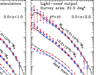
Refer to caption — Figure 1.: Two-point correlation functions of halos on the light-cone; simulation results (symbols; open circles and filled triangles for real and redshift spaces, respectively) and our predictions (solid and dotted lines for real and redshift spaces, respectively). The error bars denote the standard deviation computed from 200 random re-samplings of the bootstrap method. The amplitudes of $\xi^{LC}$ for $M_{\rm halo}\geq 5.0\times 10^{13}h^{-1}M_{\odot}$ are increased by an order of magnitude for clarity.

Figure 1 compares our model predictions with the clustering of simulated halos from “light-cone output” of the Hubble Volume $\Lambda$ CDM simulation (Evrard et al. 2001) with $\Omega_{\rm b}=0.04$ , $\Omega_{\rm CDM}=0.26$ , $\sigma_{8}=0.9$ , $\Omega_{\Lambda}=0.7$ and $h=0.7$ . For the dark matter correlation functions, our model reproduces the simulation data almost perfectly at $R>3h^{-1}$ Mpc (see also Hamana et al. 2001a). This scale corresponds to the mean particle separation of this particular simulation, and thus the current simulation systematically underestimates the real clustering below this scale especially at $z>0.5$ . Our model and simulation data also show quite good agreement for dark halos at scales larger than $5h^{-1}$ Mpc. Below that scale, they start to deviate slightly in a complicated fashion depending on the mass of halo and the redshift range. This discrepancy may be ascribed to both the numerical limitations of the current simulations and our rather simplified model for the halo biasing. Nevertheless the clustering of clusters on scales below $5h^{-1}$ Mpc is difficult to determine observationally anyway, and our model predictions differ from the simulation data only by $\sim 20$ percent at most. Therefore we conclude that in practice our empirical model provides a successful description of halo clustering on the light-cone.

4. Dark matter halos vs. galaxy clusters

With the successful empirical model of halo clustering, the next natural question is how to apply it in describing real galaxy clusters. In fact, in my opinion the main obstacle for that purpose is the lack of the universal definition of clusters. Let me give some examples that I can easily think of (see Fig.2).

(i) Press-Schechter halos:: almost all theoretical studies adopt the definition of dark matter halos according to the nonlinear spherical model. This is characterized by the mean overdensity of $18\pi^{2}$ (in the case of the Einstein - de Sitter universe. The corresponding expressions in other cosmological models can be also derived.). Combining this definition with the Press-Schechter theory, the mass function of the dark halos can be computed analytically. This makes it fairly straightforward to compare the predictions in this model with observations, and therefore this definition has been widely studied in cosmology.
(ii) Halos identified from N-body simulations:: in reality the gravitationally bound objects in the universe quite often show significant departure from the spherical symmetry. Such non-spherical effects can be directly explored with N-body simulations. Even in this methodology, the identification of dark halos from the simulated particle distribution is somewhat arbitrary. A most conventional method is the friend-of-friend algorithm. In this algorithm, the linking length is the only adjustable parameter to controle the resulting halo sample. Its value is usually set to be 0.2 times the mean particle separation in the whole simulation which qualitatively corresponds to the overdensity of $18\pi^{2}$ as described above.
(iii) Abell clusters:: until recently most cosmological studies on galaxy clusters have been based on the Abell catalogue. While this is a really amazing set of cluster samples, the eye-selection criteria applied on the Palomar plates are far from objective and cannot be compared with the above definitions in a quantitative sense.
(iv) X-ray clusters:: the X-ray selection of clusters significantly improves the reliability of the resulting catalogue due to the increased signal-to-noise and moreover removes the projection contamination compared with the optical selection. Nevertheless the quantitative comparison with halos defined according to (i) or (ii) requires the knowledge of gas density profile especially in the central part which fairly dominates the total X-ray emission.
(v) SZ clusters:: the SZ cluster survey is especially important in probing the high-z universe. In this case, however, the signal is more sensitive to the temperature profile in clusters than the X-ray selection, and thus one needs additional information/models for temperature in order to compare with the X-ray/simulation results.

The above consideration raises the importance to examine the systematic comparison among the resulting cluster/halo samples selected differently. In reality, this is a difficult and time-consuming task, and one might argue that we do not have to worry about such details at this point. Such an optimistic point of view may turn out to be reasonably right after all. Nevertheless it is still important, at present, to keep in mind that this simplistic assumption of “dark halos = galaxy clusters” may produce a systematic effect in the detailed comparison between observational data and theoretical models.

5. Conclusions

I have presented a phenomenological model for clustering of dark matter halos on the light-cone by combining and improving several existing theoretical models (Hamana et al. 2001b). One of the most straightforward and important applications of the current model is to predict and compare the clustering of X-ray selected clusters. In doing so, however, the one-to-one correspondence between dark halos and observed clusters should be critically examined at some point. This assumption is a reasonable working hypothesis, but we need more quantitative justification or modification to move on to precision cosmology with clusters.

I am afraid that this problem has not been considered seriously simply because the agreement between model predictions and available observations seems already satisfactory. In fact, since current viable cosmological models are specified by a set of many adjustable parameters, the agreement does not necessarily justify the underlying assumption. Thus it is dangerous to stop doubting the unjustified assumption because of the (apparent) success. I hope to examine these issues in future.

Acknowledgments.

I would like to thank Fred Lo for inviting me to this exciting and enjoyable meeting and also for great hospitality at Taiwan. The present work is based on my collaboration with T.Hamana, N.Yoshida, and A.E.Evrard. This research was supported in part by the Grant-in-Aid by the Ministry of Education, Science, Sports and Culture of Japan (07CE2002, 12640231).

References

Evrard, A.E. et al. 2001, ApJ, submitted

Hamana, T., Colombi, S., & Suto, Y. 2001a, A& A, 367, 18

Hamana, T., Yoshida, N., Suto, Y., & Evrard, A.E. 2001b, ApJ(Letters), in press

Jenkins, A. et al. 2001, MNRAS, 321, 372

Jing, Y.P. 1998, ApJ, 503, L9

Kaiser, N. 1987, MNRAS, 227, 1

Magira, H., Jing, Y.P., & Suto, Y. 2000, ApJ, 528, 30

Matarrese, S., Coles, P., Lucchin, F., & Moscardini, L. 1997, MNRAS, 286, 115

Matsubara, T., Suto, Y., & Szapudi, I. 1997, ApJ, 491, L1

Mo, H.J., & White, S.D.M 1996,MNRAS, 282, 347

Moscardini, L., Coles, P., Lucchin, & F., Matarrese, S. 1998, MNRAS, 299, 95

Nakamura, T. T., Matsubara, T., & Suto, Y. 1998, ApJ, 494, 13

Peacock, J.A., & Dodds, S.J. 1996, MNRAS, 280, L19

Sheth, R.K., & Tormen, G. 1999, MNRAS, 308, 119

Suto, Y., Magira, H., Jing, Y. P., Matsubara, T., & Yamamoto, K. 1999, Prog.Theor.Phys.Suppl., 133, 183

Taruya, A. & Suto,Y. 2000, ApJ, 542, 559

Yamamoto, K., & Suto, Y. 1999, ApJ, 517, 1

Yoshida, N., Sheth, R., & Diaferio, A. 2001, MNRAS, in press