An unusual H$\alpha$ nebula around the nearby neutron star RX~J1856.5$-$3754

We present spectroscopy and H$\alpha$ imaging of a faint nebula surrounding the X-ray bright, nearby neutron star RX~J1856.5$-$3754. The nebula shows no strong lines other than the Hydrogen Balmer lines and has a cometary-like morphology, with the apex being approximately 1″ ahead of the neutron star, and the tail extending up to at least 25″ behind it. We find that the current observations can be satisfactorily accounted for by two different models. In the first, the nebula is similar to “Balmer-dominated” cometary nebulae seen around several radio pulsars, and is due to a bow shock in the ambient gas arising from the supersonic motion of a neutron star with a relativistic wind. In this case, the emission arises from shocked ambient gas; we find that the observations require an ambient neutral Hydrogen number density $n_{\rm H^{0}}\simeq 0.8{\rm\,cm^{-3}}$ and a rotational energy loss $\dot{E}\simeq 6\times 10^{31}{\rm\,erg}{\rm\,s^{-1}}$. In the second model, the nebula is an ionisation nebula, but of a type not observed before (though expected to exist), in which the ionisation and heating are very rapid compared to recombination and cooling. Because of the hard ionising photons, the plasma is heated up to $\sim\!70000{\rm\,K}$ and the emission is dominated by collisional excitation. The cometary morphology arises arises naturally as a consequence of the lack of emission from the plasma near and behind the neutron star (which is ionised completely) and of thermal expansion. We confirm this using a detailed hydrodynamical simulation. We find that to reproduce the observations for this case, the neutral Hydrogen number density should be $n_{\rm H^{0}}\simeq 3{\rm\,cm^{-3}}$ and the extreme ultraviolet flux of the neutron star should be slightly in excess, by a factor $\sim\!1.7$, over what is expected from a black-body fit to the optical and X-ray fluxes of the source. For this case, the rotational energy loss is less than $2\times 10^{32}{\rm\,erg}{\rm\,s^{-1}}$. Independent of the model, we find that RX~J1856.5$-$3754 is not kept hot by accretion. If it is young and cooling, the lack of pulsations at X-ray wavelengths is puzzling. Using phenomenological arguments, we suggest that RX~J1856.5$-$3754 may have a relatively weak, few $10^{11}{\rm\,G}$, magnetic field. If so, it would be ironic that the two brightest nearby neutron stars, RX~J1856.5$-$3754 and RX~J0720.4$-$3125, may well represent the extreme ends of the neutron star magnetic field distribution, one a weak field neutron star and another a magnetar.

1 Introduction

From studies with the EINSTEIN X-ray satellite and the ROSAT all-sky survey, nearly a dozen bright soft X-ray sources have been identified with nearby neutron stars (Caraveo et al. 1996; Motch 2000). The list includes nearby ordinary pulsars (e.g., PSR B0656+14), a millisecond pulsar (PSR J0437$-$4715) and a gamma-ray pulsar (Geminga, likely a radio pulsar whose beam does not intersect our line of sight). Apart from these, the sample also includes six radio-quiet, soft X-ray emitting neutron stars whose origin is mysterious (Treves et al. 2000).

The emission from all six sources appears to be completely thermal. This might make it possible to derive accurate temperatures, surface gravities, and gravitational redshifts from fits to atmospheric models. Therefore, there has been growing interest in the using these neutron stars as natural laboratories for the physics of dense matter. In particular, Lattimer & Prakash (2001) show that a radius measurement good to 1 km accuracy is sufficient to usefully constrain the equation of state of dense matter.

Of the six sources, the brightest is RX~J1856.5$-$3754 (Walter et al. 1996). Walter & Matthews (1997) used the Hubble Space Telescope (HST) to identify RX~J1856.5$-$3754 with a faint blue star, for which Walter (2001) measured a distance of about 60${\rm\,pc}$ by direct trigonometric parallax. Pons et al. (2001) showed that the totality of the data (optical, UV, EUV and X-ray) can be accounted for by a neutron star with a surface temperature, $kT_{\rm eff}\simeq 50{\rm\,eV}$ and radius $\sim\!7\,(d/60{\,\rm pc})\,$km.

As yet, no pulsations have been detected for RX~J1856.5$-$3754 (Pons et al. 2001; Burwitz et al. 2001). In contrast, for the second brightest source, RX~J0720.4$-$3125, Haberl et al. (1997)) found clear pulsations, with a period of 8.39${\rm\,s}$. This source has also been identified with a faint blue star (Motch & Haberl 1998; Kulkarni & van Kerkwijk 1998). The long rotation period makes the nature of RX~J0720.4$-$3125 rather mysterious. Models that have received some considerations are a neutron star accreting from the interstellar medium and a middle-aged magnetar powered by its decaying magnetic field (ibid.; Heyl & Kulkarni 1998).

In order to be able to secure accurate physical parameters from observations of these sources, we need to understand their nature. In particular, we need to know the composition of the surface and the strength of the magnetic field. Motivated thus, we have embarked on a comprehensive observational programme on RX~J1856.5$-$3754. In our first paper (Van Kerwijk & Kulkarni 2001, hereafter Paper I), we presented the optical spectrum and optical and ultraviolet photometry from data obtained with the Very Large Telescope (VLT) and from the HST archive. We found that all measurements were remarkably consistent with a Rayleigh-Jeans tail, and placed severe limits to emission from other mechanisms such as non-thermal emission from a magnetosphere.

In this paper, the second in our series, we report upon a cometary nebula around RX~J1856.5$-$3754, which was discovered during the photometric and spectroscopic observations reported on in Paper I. We find that the nebula could be a pulsar bow shock, similar to what is seen around other pulsars, or a photo-ionisation nebula, of a type that has not yet been seen anywhere else, but which arises naturally in models of neutron stars accreting from the interstellar medium (Blaes et al. 1995). For either case, the nebula offers a number of new diagnostics: the density of the ambient gas and the three dimensional motion of the neutron star, and either a measurement of the rotational energy loss $\dot{E}$ from the neutron star, which so far has not been possible to make for lack of pulsations, or a measurement of the source’s brightness in the extreme ultraviolet, which is impossible to obtain otherwise because of interstellar extinction.

The organisation of the paper is as follows. First, in Sect. 2, we briefly summarise the relevant observed properties of RX~J1856.5$-$3754. Next, in Sect. 3, we present the details of the observations leading to the discovery of the nebula, and in Sects. 4 and 5 we investigate its nature.

Given the detailed modelling that we have undertaken, the article is necessarily long. Sect. 6 offers a summary of our results and contains a discussion of the clues about the nature of this enigmatic source offered by the discovery of the nebula. We recommend that those of less patient inclination read Sect. 6 first.

2 RX~J1856.5$-$3754

The spectral energy distribution of RX~J1856.5$-$3754 has been studied in detail by Pons et al. (2001), using optical and ultraviolet measurements from HST and soft X-ray measurements from EUVE and ROSAT. They find that the overall energy distribution can be reproduced reasonably well with black-body emission with a temperature $kT_{\infty}=48\pm 2{\rm\,eV}$, $n_{\rm{}H}=2.2^{+0.4}_{-0.3}\times 10^{20}{\rm\,cm^{-2}}$, and $R_{\infty}/d=0.11\pm 0.01{\rm\,km}{\rm\,pc^{-1}}$. The black-body model is not a very good fit to the X-ray data, which require a somewhat higher temperature and lower column ($63\pm 3{\rm\,eV}$ and $1.0\pm 0.2\times 10^{20}{\rm\,cm^{2}}$, respectively; Burwitz et al. 2001). This indicates that the real atmosphere is more complicated. Indeed, Pons et al. (2001) find that more detailed atmospheric models for compositions of ‘Si-ash’ and pure Fe give better fits. For those, however, one expects strong lines and bands, which appear not to be present in high-resolution X-ray spectra obtained with Chandra (Burwitz et al. 2001).

In Paper I, we reported VLT photometric and spectroscopic observations of RX~J1856.5$-$3754. Our VLT spectrum, over the range 4000–7000 Å, did not show any strong emission or absorption features. With considerable care to photometric calibration, we obtained photometry from VLT and archival HST imaging data. We found that over the entire optical through ultraviolet range (1500 Å–7000 Å), the spectral energy distribution was remarkably well described by a Rayleigh-Jeans tail, $f_{\lambda}\propto\lambda^{-4}$ with $A_{V}=0.12\pm 0.05$ and an unextincted spectral flux of $f_{\lambda_{0}}=(3.36\pm 0.17)\times 10^{-19}{\rm\,erg}{\rm\,s^{-1}}{\rm\,cm^{-2}}{\rm\,{\hbox{\AA}}^{-1}}$ at $\lambda_{0}=5000{\rm\,{\hbox{\AA}}}$. The reddening corresponds to $N_{H}\simeq 2.4\times 10^{20}$ cm^-2 (Predehl & Schmitt 1995), consistent with that estimated from X-ray spectroscopy (see above).

Walter (2001) used HST to measure the proper motion and parallax of RX~J1856.5$-$3754; he found $\mu=332\pm 1{\rm\,mas}{\rm\,yr^{-1}}$ at position angle $\theta=100\aas@@fstack{\circ}3\pm 0\aas@@fstack{\circ}1$ and $\pi=16.5\pm 2.3{\rm\,mas}$. The parallax corresponds to a distance of $61^{+9}_{-8}$${\rm\,pc}$. The proper motion is directed away from the Galactic plane, $(\mu_{l},\mu_{b})=(63.8,-325.8){\rm\,mas}{\rm\,yr^{-1}}$, and away from the Upper Scorpius OB association. Walter suggests that RX~J1856.5$-$3754 may have been the companion of $\zeta$ Oph, which is a runaway star that likely originated in Upper Sco, but Hoogerwerf et al. (2001) argue that PSR J1932+1059 was the companion to $\zeta$ Oph. In any case, the proper motion places RX~J1856.5$-$3754 in the vicinity of Upper Sco association about a million years ago. Thus, it is quite plausible that RX~J1856.5$-$3754 was born in the Upper Sco association, in which case its age is about a million years.

The radial velocity of RX~J1856.5$-$3754 is unknown. However, assuming an origin in the Upper Sco association, it should be about $-55{\rm\,km}{\rm\,s^{-1}}$ (Walter 2001). If so, the angle between the plane of the sky and the velocity vector is $i\simeq 60\degr$. However, the radial velocity (and thus $i$) does depend on the distance of RX~J1856.5$-$3754. For instance, if the distance is 100 pc, then the radial velocity required for an origin in Upper Sco is about $-20{\rm\,km}{\rm\,s^{-1}}$.

3 Observations

In 1999 June, we used the VLT to obtain optical spectra of RX~J1856.5$-$3754. The reduction of these data and the resulting spectra are described in detail in Paper I. In the spectra, we discovered extended H$\alpha$ and H$\beta$ emission around the source. We formed spectral images along the two slits which we used for the observations – one roughly along the proper motion direction and another roughly perpendicular to it (over stars F and L, respectively; see Fig. 2 and Fig. 1 in Paper I). From these images, it was clear that the nebula is most extended along the path that the object has taken.

3.1 Nebular spectrum

In Fig. 1, we show the spectrum of the nebula. This was formed by extracting a region of 2″ around RX~J1856.5$-$3754 from the spectral images for both slits, subtracting the contribution from RX~J1856.5$-$3754, and averaging the two weighted by the exposure time. The flux calibration was done with the help of an exposure of the standard star EG 274 (Paper I). From the figure, it is clear that no other lines than H$\alpha$ and H$\beta$ are observed. The slightly elevated continuum at longer wavelengths reflects an increased contribution of an extended source near the neutron star (see below).

Figure 1: Spectrum of the nebula around RX~J1856.5$-$3754, showing emission in H$\alpha$ and H$\beta$, but not in any other lines. The continuum emission from RX~J1856.5$-$3754 has been subtracted. The slight rise in the continuum to longer wavelengths is due to a faint, red extended object close to RX~J1856.5$-$3754 (see Sect. 3.2 and Fig. 2).

3.2 H$\alpha$ image

To study the nebula in more detail, follow-up H$\alpha$ imaging was done for us in Service time with the VLT in May 2000. In addition, deep B and R-band images were obtained. The reduction of these images and the B and R-band photometry are described in Paper I. The reduced H$\alpha$ image is shown in Fig. 2. In order to bring out diffuse emission better, we also show an image in which the stars have been removed by point–spread function fitting (which was produced in the process of doing photometry with daophot; see below). Apart from the faint H$\alpha$ nebula (inside the box), also more extended diffuse emission is present. The latter also appears in our B- and R-band images and hence does not reflect H$\alpha$ emission, but more likely scattered light, perhaps due to dust associated with the R CrA complex.

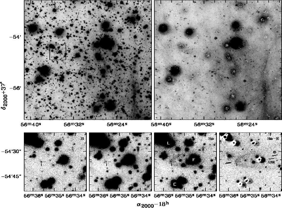
Figure 2: Images of RX~J1856.5$-$3754, its nebula, and the field. The upper-left panel gives an overview of the stacked H$\alpha$ image. In the upper-right panel, all but the most overexposed stars have been removed using point-spread function fitting. Except for the nebula (inside the box in the upper-left panel), all diffuse emission that is seen has matching emission in the B and R images, indicating that it is due to scattered light. The lower row of panels shows enlargements of the area inside the box in the upper-left panel, in B, R, H$\alpha$ and H$\alpha-{}$R. In the H$\alpha$ image, stars L, C, and F are indicated. For the H$\alpha-{}$R image, the R-band image has been optimally matched to and subtracted from the H$\alpha$ image in order to remove the contribution from broad-band light. The tick marks indicate the position of RX~J1856.5$-$3754, as measured from the B-band image. In the R-band image, one sees that there are two objects close to it. One, about $1\aas@@fstack{\prime\prime}3$ to the ESE, has been detected as well in the F606W WFPC2 images taken with HST (Walter 2001; star 115). The other, about $0\aas@@fstack{\prime\prime}9$ to the NE, is extended and only barely visible in the HST images. These objects give a false impression of a bright head of the nebula in the H$\alpha$ image; this impression disappears in the H$\alpha-{}$R image. In the H$\alpha-{}$R image, the proper motion is indicated by the longer dashes, which connect the positions the object had between 60 and 70 years ago and will have in 10 to 20 years from now. The dash marked ‘$\odot$’ shows the proper motion as seen from the Sun, while that marked ‘LSR’ shows the proper motion as seen by an observer moving with the local standard of rest (and therewith moving with the interstellar medium local to the neutron star; see Sect. 3.3).

Figure 2 also shows enlargements around RX~J1856.5$-$3754. While the nebula is clearly visible in the H$\alpha$ image, it is hard to judge its extent because of the crowded field. Furthermore, a faint star and small extended object distort the shape of the nebula’s head (the latter also contributes to the long-wavelength continuum of the nebular spectrum shown in Fig. 1).

We tried to remove the contribution of broad-band sources by subtracting a suitably scaled version of the R-band image. For this purpose, we used the image differencing technique of Alard & Lupton (1998), in which the better-seeing image of a pair (in our case, the R-band image) is optimally matched to the worse-seeing image (H$\alpha$) before the difference is taken. The matching is done by constructing a kernel, convolved with which the PSF of the better-seeing image matches the PSF of worse-seeing image optimally (in a $\chi^{2}$ sense). The resulting H$\alpha-{}$R difference image, shown in Fig. 2, is not perfect, partly because of differences in the H$\alpha$ to R flux ratios for different objects, and partly because of internal reflections in the H$\alpha$ filter, which lead to low-level, out-of-focus images near every object. Nevertheless, the nebula can be seen more clearly, and in particular the confusion near the head is greatly reduced. The nebula has a cometary shape and is somewhat edge-brightened.

3.3 Orientation

From Fig. 2, it is clear that the nebula is aligned almost, but not precisely with the proper motion of RX~J1856.5$-$3754: the position angle of the nebular axis is $97\degr\pm 1\degr$, while the position angle of the proper motion is $100\aas@@fstack{\circ}3\pm 0\aas@@fstack{\circ}1$ (Sect. 2). This slight but significant offset is not surprising, because the shape and orientation of the nebula is determined not by the motion of the neutron star relative to the Sun, but by its motion relative to the surrounding medium.

For the ambient interstellar medium, it is reasonable to assume that its velocity is small relative to the local standard of rest. If so, as observed from the Sun, the medium will have an apparent proper motion $\mu^{\rm ap}$ and radial velocity $v^{\rm ap}_{\rm rad}$, given by

$$\mu^{\rm ap}_{l} = \frac{1}{d}\left[U_{\odot}\sin l-V_{\odot}\cos l\right],$$

$$\mu^{\rm ap}_{b} = \frac{1}{d}\left[(U_{\odot}\cos l+V_{\odot}\sin l)\sin b-W_{\odot}\cos b\right],$$ (1)

$$v^{\rm ap}_{\rm rad} = -(U_{\odot}\cos l+V_{\odot}\sin l)\cos b-W_{\odot}\sin b,$$

where $(l,b)=(-1\aas@@fstack{\circ}40,-17\aas@@fstack{\circ}22)$ are the Galactic longitude and latitude of RX~J1856.5$-$3754, and $(U,V,W)_{\odot}=(10.00,5.25,7.17){\rm\,km}{\rm\,s^{-1}}$ the velocity of the Sun relative to the local standard of rest (Dehnen & Binney 1998). Inserting the numbers, we find $(\mu^{\rm ap}_{l},\mu^{\rm ap}_{b})=(-19.3,-36.2)d_{60}^{-1}{\rm\,mas}{\rm\,yr^{-1}}$ and $v^{\rm ap}_{\rm rad}=-7{\rm\,km}{\rm\,s^{-1}}$.

With the above, the proper motion of RX~J1856.5$-$3754 relative to the nebula, and therewith, by assumption, relative to the local standard of rest, is $(\mu^{\rm lsr}_{l},\mu^{\rm lsr}_{b})=(83.1,-289.7){\rm\,mas}{\rm\,yr^{-1}}$ for $d=60{\rm\,pc}$. This implies a total proper motion $\mu^{\rm lsr}=301.4\,{\rm\,mas}{\rm\,yr^{-1}}$ at position angle $\theta=95\aas@@fstack{\circ}3$; the latter is close to the angle observed for the nebular axis (Fig. 2). The implied relative spatial velocity on the sky is $v^{\rm lsr}_{\mu}=86{\rm\,km}{\rm\,s^{-1}}$, while the relative radial velocity and total velocity, assuming an origin in the Upper Scorpius association, are $v^{\rm lsr}_{\rm rad}\simeq-50{\rm\,km}{\rm\,s^{-1}}$ and $v^{\rm lsr}_{\rm tot}=100{\rm\,km}{\rm\,s^{-1}}$.

3.4 Flux calibration

No H$\alpha$ calibration images of emission-line objects were taken, and therefore we used our carefully calibrated spectra of stars F, L, and C (Paper I) to estimate the throughput. For this purpose, we measured instrumental magnitudes on our H$\alpha$ images, using daophot (Stetson 1987) in the same way as was done for B and R in Paper I, and compared these with the expected magnitudes,

$$m_{\alpha}=-2.5\log\int A_{\rm UT}R_{\alpha}(\lambda)R_{\rm open}(\lambda)\frac{\lambda}{hc}f_{\lambda}(\lambda)\,{\rm d}\lambda,$$ (2)

where $A_{\rm UT}=51.2{\rm\,m^{2}}$ is the telescope area, $R_{\alpha}$ is the response of the H$\alpha$ filter, $R_{\rm open}$ the combined response of all other elements (atmosphere, telescope, collimator, detector), and $f_{\lambda}(\lambda)$ the spectrum of the object in wavelength units. For $R_{\alpha}$, we use the response curve from the ESO web site, as measured in the instrument using a grism; the filter has a peak throughput of $\sim\!65\%$ and full width at half maximum of 60 Å. We infer a total efficiency for all other components of $R_{\rm open}=32\pm 1\%$ (assuming $R_{\rm open}$ does not vary strongly over the H$\alpha$ bandpass; we verified that a similar analysis for the R band gives a consistent result). Here, the uncertainty includes in quadrature a 2% uncertainty in the flux calibration of stars L, C, and F. For the conversion from H$\alpha$ count rates to photon rates, therefore, only the filter efficiency at H$\alpha$ is required. We find $R_{\alpha}(\lambda_{\alpha})=60\pm 5\%$, where the relatively large uncertainty stems from the fact that there is some dependence of the filter characteristics on position on the detector (even though the interference filters are located in the convergent beam).

Figure 3: Flux-calibrated H$\alpha$ images and cross cuts of the nebula around RX~J1856.5$-$3754. The lower-left panel shows the nebula, using coordinates relative to the neutron star, with the horizontal axis representing the major axis of symmetry of the nebula. In the upper-left panel, the surface brightnesses along the axis of symmetry of the nebula are shown. The points with error bars represent the H$\alpha$, H$\beta$, and H$\gamma$ brightnesses inferred from the spectra taken with the slit positioned over star F, very close to the axis of symmetry; these are marked as ‘$\alpha$,’ ‘$\beta$,’ and ‘$\gamma$,’ respectively. See Fig. 2 and Fig. 1 in Paper I for star designations including star F. The nebula is faint in H$\beta$ and undetectable in H$\gamma$. All points are averages over 3-pixel (0$\aas@@fstack{\prime\prime}$6) intervals along the slit. The thin lines indicate the zero level and show the point-spread function of star F (also averaged over 3 pixels). For H$\alpha$, it also shown at the position of RX~J1856.5$-$3754. The histogramme represents H$\alpha$ measurements inferred from the H$\alpha-{}$R image, by averaging over the numerical slit marked ‘z’ in the upper-right panel; its zero level is again indicated by a thin line. The grey scale used in the images is next to the upper-left and above the lower-right panels. In the lower-right panel, the cross cuts perpendicular to the axis of symmetry are shown. The points with error bars represent the brightnesses inferred from the spectra taken with the slit positioned over star L, and the histogrammes those inferred from the image, by integrating along numerical slits marked ‘p,’ ‘q,’ ‘r,’ and ‘s.’ The zero levels and point-spread functions are indicated by thin lines. Also displayed in the upper-right panel is the expected shape for a bow-shock (see Sect. 4).

3.5 Results

In Fig. 3, we show the calibrated H$\alpha-{}$R image, rotated such that its axis of symmetry is horizontal (assuming a position angle of $97\degr$, see Sect. 3.3). Note that the level of the background remains somewhat uncertain; indeed, it is the limiting factor in the resulting H$\alpha$ fluxes. Also shown in the Figure are cross-cuts through the image, one along the axis of symmetry, and four across it at different distances from the head of the nebula. Furthermore, the H$\alpha$, H$\beta$, and H$\gamma$ surface brightnesses inferred from the spectra are shown. The H$\alpha$ brightnesses were derived from the spectral images, by integrating over the wavelength range of 6554–6570 Å and subtracting the average of the integrated fluxes in wavelength ranges 6496–6550 and 6574–6628 Å. The H$\beta$ and H$\gamma$ surface brightnesses were determined similarly. Note that the H$\alpha$ surface brightnesses inferred from the spectra are more certain than those inferred from the H$\alpha$ image, since they suffer much less from uncertainties in the background level.

The nebula is clearly resolved in all directions. It reaches half-maximum brightness $1\aas@@fstack{\prime\prime}0\pm 0\aas@@fstack{\prime\prime}2$ in front of the neutron star, about $2\arcsec$ to each side, and $\sim\!3\arcsec$ behind the neutron star. The tail is visible to at least $25\arcsec$ behind the neutron star. The peak surface brightness of the nebula is $1.3\times 10^{-17}{\rm\,erg}{\rm\,s^{-1}}{\rm\,cm^{-2}}{\rm\,arcsec^{-2}}$, corresponding to a photon rate of $4.3\times 10^{-6}{\rm\,s^{-1}}{\rm\,cm^{-2}}{\rm\,arcsec^{-2}}$.

Below we discuss the origin of this nebula and see if we can use it to shed additional light on the nature of the enigmatic object, RX~J1856.5$-$3754.

4 A pulsar bow shock?

Cometary nebulae shining in the Balmer lines (with no detectable lines from any other element) have been seen around a number of pulsars. The accepted physical model for such nebulae is the pulsar bow-shock model, which was invoked first by Kulkarni & Hester (1988) to explain a similar H$\alpha$ nebula around the binary millisecond pulsar PSR B1957+20. Thus, both the similarity of the nebula to nebulae seen around some pulsars, as well as the reasonable possibility that RX~J1856.5$-$3754 is a million-year old neutron star (see Sect. 2) and thus might be a pulsar, motivate us to consider the bow-shock model.

4.1 Stand-off distance and shape

Consider a pulsar moving supersonically through partially ionised interstellar medium of density $\rho_{\rm ism}$. Along the direction of motion the medium ram pressure is $\rho_{\rm ism}v_{\rm ns}^{2}$, where $v_{\rm ns}$ is the speed of the pulsar. At the apex of the nebula, the (quasi) spherical relativistic pulsar wind is balanced by this ram pressure at a “stand-off” distance $r_{\rm a}$, where

$$\frac{\dot{E}}{4\pi r_{\rm a}^{2}c}=\rho_{\rm ism}v_{\rm ns}^{2}.$$ (3)

Here, $\dot{E}$ is the luminosity in the relativistic wind, which is assumed to be primarily in the form of relativistic particles and magnetic fields. By considering momentum balance along other directions, Wilkin (1996) derived an analytic solution for the shape of the nebula,

$$r_{\theta}\sin\theta=r_{\rm a}\sqrt{3\left(1-\frac{\theta}{\tan\theta}\right)}.$$ (4)

Note that in this derivation it is assumed that the shocked gas cools rapidly, so that thermal pressure is negligible (a two-dimensional equivalent to the ‘snow-plough’ phase in supernova remnants). If this assumption is incorrect then the tail should be slightly wider.

4.2 Shock emission mechanisms

Along the cometary surface, one expects two shocks, with in between an inner region consisting of shocked pulsar wind and an outer region of shocked interstellar medium. The former will shine primarily via synchrotron emission and is best searched for at X-ray (e.g. the Mouse, Predehl & Kulkarni 1995) or radio wavelengths (see Gaensler et al. 2000 for a review of radio searches).

All astrophysical shocks appear to be collisionless and mediated via ionised particles. Thus, the ambient neutral particles (i.e., atoms) do not notice the shock, but do find themselves subjected to collisional excitation and ionisation by shocked electrons and to charge exchange with shocked protons (Chevalier & Raymond 1978; Raymond 1991). Both these processes can lead to line emission. Electronic excitation of the unshocked neutrals will result in a narrow line, reflecting the velocity dispersion of the unshocked gas. Charge exchange of a Hydrogen atom with a fast-moving proton will result in a Hydrogen atom having the velocity of the shocked proton and its H$\alpha$ emission will reflect the large velocity dispersion and the bulk velocity of the shocked protons (Chevalier & Raymond 1978; Raymond 1991). Elements other than Hydrogen will also be excited collisionally, but the large abundance of hydrogen and the high temperature ensure that the emitted optical spectrum is dominated by hydrogen lines. Hence, the name “Balmer-dominated” shocks.

Balmer-dominated shocks are rare because two stringent conditions need to be met. First, the ambient ISM has to be (partially) neutral. Second, the shock has to be “young.” The latter condition arises from the fact that for shock speeds greater than 110${\rm\,km}$${\rm\,s^{-1}}$, the post-shock gas, if allowed sufficient time to cool, produces so much ionising flux that the pre-shocked ambient gas ahead of the shock front becomes almost completely ionised (Shull & McKee 1979; McKee & Hollenbach 1980). Thus, Balmer-dominated shock spectra are expected only in shocks which have not enough time to sweep a “cooling column” density, $N_{\rm cool}=1.8\times 10^{16}v_{100}^{3.6}{\rm\,cm^{-2}}$ (Hartigan et al. 1987); here, $v_{100}$ is the shock speed in units of $100{\rm\,km}{\rm\,s^{-1}}$.

Given this reasoning, it might come as a surprise that Balmer-dominated bow shocks have been found around pulsars with a wide variety of ages (Kulkarni & Hester 1988; Cordes et al. 1993; Bell et al. 1995). Pulsar bow shocks are far from planar, however, and as a result the shocked material subtends an ever decreasing solid angle as seen from the vantage point of the stand-off region. In addition, pulsars spend most of their time moving through diffuse interstellar medium and thus matter recombines only far behind the pulsar. The combination of both reasons ensures Balmer-dominated pulsar bow shocks can form.

4.3 Application to RX~J1856.5$-$3754

Turning now to RX~J1856.5$-$3754, we start by noting that the shape of the nebula fits reasonably well with the expression given by Eq. 4, as can be seen in Fig. 3. By trying different inclinations $i$ and projected angular stand-off distances $\theta_{\parallel}$, we find a best match around $i=60\degr$ and $\theta_{\parallel}=1\aas@@fstack{\prime\prime}0$, with a ‘chi-by-eye’ uncertainty of about $15\degr$ and $0\aas@@fstack{\prime\prime}2$, respectively. This determination is consistent with our inference of the radial velocity with respect to the local medium (see Sect. 2). Note, however, that, as mentioned above, Eq. 4 is derived under the assumption of rapid radiative cooling; if this is not met, the tail would be wider and hence the observations would imply inclinations closer to $90\degr$. We return to this aspect below.

In the framework of the bow-shock model, apart from the orientation, there are four unknowns, the relative velocity, the pulsar wind energy loss $\dot{E}$, the interstellar medium density $\rho_{\rm ism}$, and the fraction $\xi_{0}=n_{\rm H^{0}}/n_{\rm H}$ of the neutral ambient gas. In contrast, we have only three measurements: the velocity, the observed H$\alpha$ flux, $n_{\alpha}$, and the angular distance between the neutron star and the apex of the cometary nebula, $\theta_{\parallel}$. The physical length of the standoff distance is $r_{\rm a}=d\theta_{\parallel}/\sin{i}=60d_{60}/\sin{i}{\rm\,AU}$, where $d_{60}$ is the distance in units of 60${\rm\,pc}$. For simplicity, we will drop the dependence on $\sin i$ in our estimates below, and will take $v_{\rm ns}=d\mu_{\rm ns}=100d_{60}{\rm\,km}{\rm\,s^{-1}}$.

The H$\alpha$ flux is proportional to the incoming flux of neutral particles (H i atoms). Raymond (1991) states that for a broad range of shock velocities, about 0.2 H$\alpha$ photons are produced per neutral particle before that particle is ionised in the post-shock region. Unfortunately, there are few calculation for the yield of H$\alpha$, the number of H$\alpha$ photons per incoming neutral atom, $f_{\alpha}$, for low velocity shocks, $\sim\!100{\rm\,km}{\rm\,s^{-1}}$. According to Cox & Raymond (1985), for a $120{\rm\,km}{\rm\,s^{-1}}$ shock, $f_{\alpha}\simeq 0.1$ for case A (i.e., most higher order Lyman photons, Ly$\beta$, Ly$\gamma$, etc., escape from the shocked region) or $\sim\!0.23$ for case B (higher order Lyman photons are absorbed locally and re-emitted until they are converted; e.g., to H$\alpha$ and two-photon continuum for Ly$\beta$). We will assume case A and normalise the yield accordingly: $f_{\alpha}=0.1f_{\alpha,0.1}$.

Considering the head of the nebula only, the expected number of H$\alpha$ photons is related to the other parameters as follows:

$$n_{\alpha}=\frac{f_{\alpha}n_{\rm H^{0}}\pi r_{\perp}^{2}v_{\rm ns}}{4\pi d^{2}}=\frac{1}{4}f_{\alpha}n_{\rm H^{0}}\theta_{\perp}^{2}\mu_{\rm ns}d.$$ (5)

Here, $r_{\perp}$ is the radius of the bow shock perpendicular to the axis of symmetry and $\theta_{\perp}=r_{\perp}/d$ the corresponding angular distance.

With $\theta_{\perp}=2\arcsec$, the measured $\mu_{\rm ns}$ (Sect. 3) and the observed H$\alpha$ photon rate of $n_{\alpha}\simeq 2\times 10^{-5}{\rm\,s^{-1}}{\rm\,cm^{-2}}$, we find

$$n_{\rm H^{0}}=0.8{\rm\,cm^{-3}}\;f_{\alpha,0.1}^{-1}d_{60}^{-1}.$$ (6)

Noting that the total density of the ambient gas is $\rho_{\rm ism}=n_{\rm H^{0}}m_{\rm H}X^{-1}\xi_{0}^{-1}$, where $X=0.73$ is the fraction of hydrogen by mass and $\xi_{0}=n_{\rm H^{0}}/n_{\rm H}$ is the neutral fraction, and applying Eq. 3, we find,

$$\dot{E}\simeq 6\times 10^{31}{\rm\,erg}{\rm\,s^{-1}}\;f_{\alpha,0.1}^{-1}{\xi_{0}}^{-1}d_{60}^{3}.$$ (7)

We find that because we have fewer measurements than unknowns, we are only able to constrain the quantity $\xi_{0}\dot{E}$. Since $\xi_{0}\leq 1$, we obtain a lower limit to $\dot{E}$.

If, as argued above, RX~J1856.5$-$3754 is a $t=10^{6}t_{6}{\rm\,yr}$ old pulsar, then assuming that the main energy loss is due to magnetic dipole radiation (magnetic field strength $B$, braking index $n=3$), we can apply the usual relations, $\tau_{\rm char}\equiv P/2\dot{P}=t/\chi$, with $\chi=1-(P_{0}/P)^{2}\simeq 1$ (where $P$ and $P_{0}$ are the current and birth period, respectively), $\dot{E}=I4\pi^{2}\dot{P}/P^{3}=I4\pi^{2}/2\tau P^{2}$ (where $I=10^{45}I_{45}{\rm\,g}{\rm\,cm^{2}}$ is the moment of inertia), and $B=3.2\times 10^{19}(P\dot{P})^{1/2}=3.2\times 10^{19}P/(2\tau)^{1/2}{\rm\,G}$, to obtain,

$$P \simeq 3.3{\rm\,s}\;\chi^{1/2}I_{45}^{1/2}t_{6}^{-1/2}f_{\alpha,0.1}^{1/2}\xi_{0}^{1/2}d_{60}^{3/2},$$ (8)

$$B \simeq 1.3\times 10^{13}{\rm\,G}\;\chi I_{45}^{1/2}t_{6}^{-1}f_{\alpha,0.1}^{1/2}\xi_{0}^{1/2}d_{60}^{3/2}.$$ (9)

Since $\chi\leq 1$ and $\xi_{0}\leq 1$, the values of $B$ and $P$ are true upper limits. The limits on $B$ and $P$ are consistent with those expected from ordinary million-year old pulsars. Thus, the bow-shock model appears to provide a reasonable description of the nebula we observe.

4.4 Consistency checks

We now verify that the bow-shock model is consistent with the assumptions we made. First, the shape of the bow shock was assumed to be specified by Eq. 4 and this assumption implicitly requires that the shock radiate much of the energy. How good is this assumption? Every H i atom comes into the shocked region with an energy of $\frac{1}{2}m_{\rm H}v_{\rm ns}^{2}\simeq 60v_{\rm ns,100}^{2}{\rm\,eV}$ where $v_{\rm ns,100}$ is the shock speed in units of $100{\rm\,km}{\rm\,s^{-1}}$. Of this, about $\frac{7}{16}$ goes into shock heating and the remainder into bulk motion. Only one out of five hydrogen atom are excited to the $n=3$ level before being ionised; including other levels, likely the energy loss from the shocked region is $\sim\!2\times 13.6{\rm\,eV}$ per neutral. Thus the ratio of energy radiated to the incoming kinetic energy is $\sim\!1.0\xi_{0}$. Thus, the use of a “snow-plough” approximation is not unreasonable. This is supported observationally by the fact that the three pulsar bow shocks studied to date, in particular the two with velocities comparable to that of RX~J1856.5$-$3754 (PSR B1957+20, Kulkarni & Hester (1988); PSR J0437$-$4715, Bell et al. (1995)), display nebulae with sharp boundaries.

Second, the ambient gas has to be partially neutral in order to see Balmer line emission. The inferred Hydrogen number density of $\sim\!1{\rm\,cm^{-3}}$ is not an unreasonable density (in order) for the Warm Neutral Medium (WNM) or the Warm Ionised Medium (WIM). The two phases taken together are expected to occupy 50% of interstellar space locally; see Kulkarni & Heiles (1988) and Dickey & Lockman (1990) for general reviews of the conditions in the interstellar medium. The ionisation in the WNM is low but the WIM is partially ionised, $\xi_{0}\sim 0.5$ (see Reynolds et al. 1995; Redfield & Linsky 2000).

Independent of the nature of the ambient gas, the bow-shock model requires that the incoming gas not be fully ionised by the extreme ultra-violet radiation from RX~J1856.5$-$3754. In the next section, we treat the case of a pure ionisation nebula. We find that the ambient gas is becomes half-ionised at an angular offset, in the forward direction of only $\sim\!0\aas@@fstack{\prime\prime}2f_{\rm bb}$ (Eq. 20) where $f_{\rm bb}$ is the excess of ionising flux (in the extreme ultraviolet band) over that expected from blackbody fits to the X-ray and optical data of RX~J1856.5$-$3754. Thus we would have to abandon the pulsar bow shock model if $f_{\rm bb}\ga 4$.

Third, in our estimates, we implicitly assumed the bow-shock was thin compared to the distance to the neutron star. Ghavamian et al. (2001) have computed the ionisation structure of Balmer-dominated shocks for $n_{\rm H^{0}}=1{\rm\,cm^{-3}}$ and $\xi_{0}=0.5$. For a $250{\rm\,km}{\rm\,s^{-1}}$ shock, they find that the time scale on which an H i is ionised by electrons is $0.2{\rm\,yr}$, and that the time scale on which proton charge exchange becomes ineffective is about $\sim\!0.4{\rm\,yr}$. These time scales are expected to depend only weakly on velocity and to be inversely proportional to density. The corresponding length scales are $l\simeq 10^{14}v_{\rm ns,100}{\rm\,cm}$, which is smaller than $r_{\rm a}\simeq 10^{15}d_{60}{\rm\,cm}$. Thus, we conclude that the assumption of a thin bow shock is reasonable.

Finally, we verify whether the assumption of case A was reasonable. For the Lyman lines, the line-centre cross-section is given by (Rybicki & Lightman 1979)

$$\alpha_{\nu_{0},1,n} = \frac{\pi e^{2}}{m_{\rm e}c}f_{1,n}\frac{c}{\nu_{0}}\sqrt{\frac{m_{\rm H}}{2\pi kT}}$$ (10)

$$= 1.16\times 10^{-14}{\rm\,cm^{2}}\;\lambda_{0,\hbox{\scriptsize\AA}}f_{1,n}T_{\rm K}^{-1/2},$$

where $f_{1,n}$ is the oscillator strength (for Ly$\beta$ through Ly$\epsilon$, $f_{1,2\ldots 5}=0.4162$, 0.07910, 0.002899, and 0.001394). The line-centre optical depth in the Ly$\beta$ line is thus $\sim\!2\times\alpha_{\nu_{0},1,1}n_{\rm H^{0}}l\simeq 0.8$; here the multiplicative factor of 2 is a crude approximation to account for the bow shock geometry. Since in every absorption, there is a probability of only 0.118 that Ly$\beta$ is converted to H$\alpha$ (plus two-photon continuum), we conclude that our assumption of case A is reasonable.

5 An ionisation nebula?

RX~J1856.5$-$3754 is a source of ionising photons and, as with hot white dwarfs, should have an ionised region around it. Such a region would produce H$\alpha$ emission, and would be deformed because of the proper motion of the neutron star. Indeed, Blaes et al. (1995) showed that isolated neutron stars accreting from the interstellar medium should have associated H$\alpha$ nebulae with cometary shape.

To see whether ionisation could be important for the nebula around RX~J1856.5$-$3754, we will first make analytical estimates in Sect. 5.1, following the analysis of Blaes et al. (1995). We will find that ionisation could lead to a nebula with properties in qualitative agreement with the observations. The inferred conditions in the nebula, however, are rather different from those encountered in “normal” ionisation nebulae; we discuss this briefly in Sect. 5.2. Next, in Sect. 5.3, we present a detailed simulation with which we attempt to reproduce the observations quantitatively.

5.1 Analytical estimates

In general, the properties of ionisation nebulae are determined by the balance between ionisation, recombination, heating and cooling. In order to determine the relative importance of these processes, we first compare their characteristic timescales with the crossing time, i.e., the time in which the neutron star with velocity $v_{\rm ns}$ moves a distance equal to the distance $r_{\rm a}$ to the apex of the nebula,

$$t_{\rm cross}=\frac{r_{\rm a}}{v_{\rm ns}}=\frac{\theta_{\rm a}}{\mu_{\rm ns}}=3{\rm\,yr}.$$ (11)

For our analytical estimates here and below we take $r_{\rm a}=d\theta_{\rm a}\simeq 9\times 10^{14}d_{60}{\rm\,cm}$ and $v_{\rm ns}=d\mu_{\rm ns}\simeq 100d_{60}{\rm\,km}{s^{-1}}$, i.e., we ignore the effects of changes in inclination and the difference between observed proper motion and motion relative to the local interstellar medium discussed in Sect. 3.3. We will also assume pure Hydrogen gas. We will include Helium and use the correct geometry in the numerical model described in Sect. 5.3.

5.1.1 Ionisation and recombination timescales

The typical time for a neutral particle at the apex of the bow shock to be ionised by the emission from the neutron star is

$$t_{\rm ion}=\left(\frac{N_{\rm X}}{4\pi r_{\rm a}^{2}}\alpha_{\rm ion}\right)^{-1}=\left(\frac{n_{\rm X}\alpha_{\rm ion}}{\theta_{\rm a}^{2}}\right)^{-1},$$ (12)

where $N_{\rm X}$ is the rate at which ionising photons are emitted, $n_{\rm X}=N_{\rm X}/4\pi d^{2}$ the rate at which these would arrive at Earth in the absence of interstellar absorption, and $\alpha_{\rm ion}$ the effective cross section for ionisation of Hydrogen. The latter is given by

$$\alpha_{\rm ion}=\frac{\int_{\nu_{\rm ion}}^{\infty}\alpha_{\nu}(S_{\nu}/h\nu)\,{\rm d}\nu}{\int_{\nu_{\rm ion}}^{\infty}(S_{\nu}/h\nu)\,{\rm d}\nu}\simeq 1.4\times 10^{-19}{\rm\,cm^{2}}\;T_{\rm ns,50}^{-1.67};$$ (13)

here $S_{\nu}$ is the surface emission, which for the numerical estimate is assumed to be a black-body with temperature $kT_{\rm eff}=50T_{\rm ns,50}{\rm\,eV}$. For this cross section, the effective optical depth $\tau=n_{\rm H^{0}}\alpha_{\rm ion}r_{\rm a}\simeq 1.3\times 10^{-4}n_{\rm H^{0}\!,1}$ is very small (here $n_{\rm H^{0}}=1n_{\rm H^{0}\!,1}{\rm\,cm^{-3}}$ is the neutral Hydrogen number density). Even the optical depth at the Lyman edge is small: $\alpha_{\rm edge}=6.3\times 10^{-18}{\rm\,cm^{2}}$ and hence $\tau_{\rm edge}\simeq 6\times 10^{-3}n_{\rm H^{0}\!,1}$.

We estimate $n_{\rm X}$ by scaling to the observed, de-reddened optical flux, and assuming that the emitted spectrum resembles that of a black body, i.e.,

$$n_{\rm X}=n_{\rm opt}\frac{\int_{\nu_{\rm ion}}^{\infty}(S_{\nu}/h\nu)\,{\rm d}\nu}{\int_{\rm opt}(S_{\nu}/h\nu)\,{\rm d}\nu}\simeq 0.4{\rm\,s^{-1}}{\rm\,cm^{-2}}\;f_{\rm bb}T^{2.0}_{\rm ns,50},$$ (14)

where we used the unabsorbed photon rate inferred in Paper I from the optical and ultra-violet photometry of $8.5\times 10^{-8}{\rm\,s^{-1}}{\rm\,cm^{-2}}{\rm\,{\hbox{\AA}}^{-1}}$ at 5000 Å and where $f_{\rm bb}$ is a factor which takes into account the extent to which the emitted spectrum deviates from that of a black body.

With the above estimates, we find

$$t_{\rm ion}\simeq 13{\rm\,yr}\;f_{\rm bb}^{-1}T_{\rm ns,50}^{-0.33}.$$ (15)

The typical time it takes for a proton to recombine is

$$t_{\rm rec}=\left(\alpha_{\rm rec}n_{\rm e}\right)^{-1}\simeq 10^{5}{\rm\,yr}\;n_{\rm e,1}^{-1},$$ (16)

where $\alpha_{\rm rec}$ is the recombination cross section and $n_{\rm e}=1n_{\rm e,1}{\rm\,cm^{-3}}$ the electron number density. For the estimate, we used $\alpha_{\rm rec}\simeq 4\,10^{-13}{\rm\,cm^{-3}}{\rm\,s^{-1}}$, which is for case A at $10^{4}{\rm\,K}$ (Osterbrock 1989). Case A is appropriate here, since we found above that the Lyman continuum is optically thin and thus recombination directly to the ground state does not lead to local ionisation of another atom (as is assumed in Case B, for which the recombination rate is $\sim\!40\%$ lower). We will find below that the temperature is likely substantially higher than $10^{4}{\rm\,K}$, but this will only lead to lower recombination rates.

Clearly, for any reasonable density, the recombination time scale is far longer than the crossing time. The ionisation time scale, however, is comparable to the crossing time. To match the two, $f_{\rm bb}$ will have to be somewhat larger than unity, but such a deviation may simply reflect the difference between a real neutron star atmosphere and a black body spectrum. Thus, the size of the nebula is consistent with it being due to ionisation. The tail of ionised matter will have length of $\mu_{\rm ns}t_{\rm rec}\simeq 10\degr$. This is far longer than the observed length, but we will see in Sect. 5.1.3, where we consider thermal balance and the relevant emission processes, that this difference can be understood. First, however, we calculate the ionisation structure of the head of the ionisation nebula.

5.1.2 Structure of the ionisation nebula

In general, the fraction of ionised particles $\xi_{+}=n_{\rm H}^{+}/n_{\rm H}$ changes as a function of time as

$$\frac{{\rm d}\xi_{+}}{{\rm d}t}=(1-\xi_{+})\alpha_{\rm ion}\frac{N_{\rm X}{\rm e}^{-\tau(r)}}{4\pi r^{2}}-\xi_{+}n_{\rm e}\alpha_{\rm rec}.$$ (17)

Given our estimates above, both optical depth effects and recombination can be ignored. For this case, the ionisation structure can be solved analytically. In a cylindrical coordinate system $(p,z)$ with the neutron star at the origin and gas moving by in the $+z$ direction, the solution is

$$\xi_{+}=1-\exp\left(-\frac{z_{0}}{p}\arctan\frac{p}{-z}\right),$$ (18)

where the length scale $z_{0}$ is given by

$$z_{0}=\frac{\alpha_{\rm ion}^{\rm eff}N_{\rm X}}{4\pi v_{\rm ns}},$$ (19)

and where $\arctan(p/{-z})$ – taken to be in the range $[0,\pi]$ – measures the angle with respect to the direction of the proper motion. From Eq. 18, one sees that in a parcel of interstellar matter at given impact parameter $p$, $\xi_{+}$ increases slowly at first, then more rapidly as it passes the neutron star, and finally slowly approaches its asymptotic value of $1-{\rm e}^{-\pi z_{0}/p}$. For large $p$, $\xi_{+}\propto 1/p$, as expected when integrating over a $1/r^{2}$ distribution.

The angular size corresponding to the length scale $z_{0}$ is

$$\theta_{0}=\frac{z_{0}}{d}=\frac{\alpha_{\rm ion}^{\rm eff}n_{\rm X}}{\mu_{\rm ns}}=0\aas@@fstack{\prime\prime}2\;f_{\rm bb}T_{\rm ns,50}^{0.33}$$ (20)

Like above, we find that to match the observed size, a somewhat larger ionising photon rate appears required than expected based on the observed optical and X-ray fluxes, i.e., $f_{\rm bb}>1$. We will return to this in Sect. 5.3, where we describe our more detailed modelling.

5.1.3 Thermal balance and emission process

We first ignore all cooling and calculate the temperature due to heating by the photo-ionisation. Using a typical energy $\bar{\epsilon}$ of the ionising photons of

$$\bar{\epsilon}=\frac{\int_{\nu_{\rm ion}}^{\infty}h\nu\alpha_{\nu}(S_{\nu}/h\nu)\,{\rm d}\nu}{\int_{\nu_{\rm ion}}^{\infty}\alpha_{\nu}(S_{\nu}/h\nu)\,{\rm d}\nu}\simeq 31.2{\rm\,eV}\;T_{\rm ns,50}^{0.25},$$ (21)

we find for a pure Hydrogen gas

$$T=\frac{2}{3k}\frac{\xi_{+}}{1+\xi_{+}}(\bar{\epsilon}-\chi_{1,\infty})\simeq 7\times 10^{4}{\rm\,K}\,T_{\rm ns,50}^{0.45}\frac{2\xi_{+}}{1+\xi_{+}},$$ (22)

where $\chi_{1,\infty}=13.6{\rm\,eV}$ is the ionisation potential of hydrogen.

The high inferred temperature of $\sim\!5\times 10^{4}{\rm\,K}$ for $\xi_{+}=0.5$ has an important consequence, viz., that collisional excitation and ionisation of Hydrogen are important. These processes will dominate the cooling. Furthermore, the H$\alpha$ emission will be dominated by radiative decay of collisionally excited neutrals. Below, we first estimate the density required to produce the observed H$\alpha$ brightness. Next, we use this to estimate the cooling time scale and check consistency.

The rate for collisional excitation to the $n=3$ level is $n_{\rm e}n_{\rm H^{0}}q_{1,3}=\xi_{+}(1-\xi_{+})n_{\rm H}^{2}q_{1,3}$, with the rate coefficient $q_{1,3}$ given by (see Osterbrock 1989)

$$q_{1,3}=\Upsilon_{1,3}\frac{2\sqrt{\pi}\alpha ca_{0}^{2}}{\omega_{1}}\sqrt{\frac{\chi_{1,\infty}}{kT}}\;{\rm e}^{-\chi_{1,3}/kT},$$ (23)

where $\Upsilon_{1,3}$ is the sum of collision strengths to the 3s, 3p, and 3d states, $\omega_{1}=2$ the statistical weight of the ground state, $\chi_{1,3}=12.1{\rm\,eV}$ the excitation potential, and $2\sqrt{\pi}\alpha ca_{0}^{2}=2.1716\times 10^{-8}{\rm\,cm^{3}}{\rm\,s^{-1}}$. The collision strength varies slowly, from $\Upsilon_{1,3}=0.25$ at $10^{4}{\rm\,K}$ to 0.43 at $7\times 10^{4}{\rm\,K}$ (Anderson et al. 2000). Inserting numbers, one finds that the largest volume emission rates are produced where $\xi_{+}\simeq 0.7$. In consequence, one expects that the emission will peak at some distance from the neutron star, and that the ionisation nebula will have a somewhat hollow appearance.

In order to estimate the hydrogen number density required to reproduce the observed brightness, we will assume case A, i.e., the medium is optically thin to Ly$\beta$ photons, so that of the excitations to the 3p state only 11.8% lead to emission of an H$\alpha$ photon (for 3s and 3d, the transition to the ground state is forbidden, so all excitations lead to H$\alpha$ emission). We label the appropriately corrected excitation rate as $q_{\alpha}^{\rm A}$. Furthermore, we will ignore excitations into higher levels which lead to H$\alpha$ photons. We consider the total H$\alpha$ photon rate integrated over the slit (with width $w_{\rm slit}=1\arcsec$) perpendicular to the proper motion. The expected rate is given by

$$n_{\alpha,\perp} \simeq \frac{\pi r_{\perp}^{2}dw_{\rm slit}n_{\rm H^{0}}n_{\rm e}q_{\alpha}^{\rm A}}{4\pi d^{2}}$$ (24)

$$= \frac{1}{4}\theta_{\perp}^{2}dw_{\rm slit}\xi_{+}(1-\xi_{+})n_{\rm H}^{2}q_{\alpha}^{\rm A}$$

$$\simeq 1.2\times 10^{-6}{\rm\,s^{-1}}{\rm\,cm^{-2}}\;d_{60}n_{\rm H,1}^{2},$$

where for the numerical estimate we used $\xi_{+}=0.5$ and $q_{\alpha}^{\rm A}\simeq 2.2\times 10^{-10}{\rm\,cm^{3}}{\rm\,s^{-1}}$ (appropriate for $T=5\times 10^{4}{\rm\,K}$). To match the observed photon rate of $1.7\times 10^{-5}{\rm\,s^{-1}}{\rm\,cm^{-2}}$ along the slit, thus requires

$$n_{\rm H}\simeq 4{\rm\,cm^{-3}}\,d_{60}^{-1/2}.$$ (25)

This is somewhat denser than the typical density of the interstellar medium or the mean density of $N_{\rm H}/d\simeq 1{\rm\,cm^{-3}}$ along the line of sight, but not by a large factor. Hence, the observed brightness can be reproduced without recourse to extreme assumptions about the interstellar medium in which the source moves.

With the above estimate of the density, we can calculate the cooling time scale and verify a posteriori that cooling is not important near the head of the nebula. As mentioned, at the high inferred temperatures, the dominant cooling processes are collisional excitation and ionisation of Hydrogen. At $T\simeq 5\times 10^{4}{\rm\,K}$, collisional excitation of the $n=2$ level is most important, with a rate coefficient $q_{1,2}\simeq 2\times 10^{-9}{\rm\,cm^{3}}{\rm\,s^{-1}}$ (Eq. 23, $\chi_{1,2}=10.2{\rm\,eV}$, $\Upsilon_{1,2}=1.4$; Anderson et al. 2000). Hence, the cooling time scale $t_{\rm cool}$ is roughly

$$t_{\rm cool} = \frac{(n_{\rm H}+n_{\rm e})\frac{3}{2}kT}{n_{\rm H^{0}}n_{\rm e}q_{1,2}\chi_{1,2}}=\frac{\bar{\epsilon}-\chi_{1,\infty}}{(1-\xi_{+})n_{\rm H}q_{1,2}\chi_{1,2}}$$ (26)

$$\simeq 14{\rm\,yr}\;n_{\rm H,4}^{-1}.$$

This time scale is a little longer than the crossing time, which confirms that temperatures as high as those inferred above can be reached. The time scale is sufficiently short, however, that more precise estimates will need to take cooling into account. We will do this in Sect. 5.3.

The relatively short cooling time scale provides the promised answer to the puzzle posed in Sect. 5.1.1: the tail appears far shorter than the recombination length of $10\degr$ because the temperature and hence the emissivity drop rapidly behind the neutron star. In principle, the tail will emit recombination radiation, but this will be at unobservable levels.

With the inferred temperatures, we can also understand why we see Balmer emission only (Fig. 1). For Helium, the temperature is too low for collisional excitation to be important. This leaves recombination and continuum pumping, neither of which are efficient enough to produce observable emission in our spectrum (see also Sect. 5.3.4). For the metals, collisional excitation may well take place, with rate coefficients comparable to or even larger than those for Hydrogen, but given their low abundances relative to Hydrogen, the resulting emission will be unobservable as well.

5.1.4 Dynamical effects

The heating due to photo-ionisation by the relatively hard photons from the neutron star will also lead to an overpressure in the gas near the neutron star relative to that further away. As a result, the gas should expand. We estimate the velocity in the direction perpendicular to the proper motion from $v_{p}=a_{p}t$, where $a_{p}$ is the acceleration associated with the pressure gradient perpendicular to the proper motion and $t$ is the time scale on which the pressure gradient changes. The acceleration is given by

$$a_{p}=-\frac{1}{\rho}\frac{{\rm d}P}{{\rm d}p}=-\frac{2}{3m_{\rm H}}\left(\bar{\epsilon}-\chi_{1,\infty}\right)\frac{{\rm d}\xi_{+}}{{\rm d}p}.$$ (27)

At $z=0$, one has ${\rm d}\xi_{+}/{\rm d}p=-(p_{0}/p^{2}){\rm e}^{-p_{0}/p}$, where $p_{0}\equiv\frac{\pi}{2}z_{0}$. The pressure gradient changes due to expansion and due to the neutron star passing by. The time scale for the latter is much faster, and is approximately given by

$$t\simeq\frac{1}{v_{\rm ns}}\left.\frac{\xi_{+}}{{\rm d}\xi_{+}/{\rm d}z}\right|_{z=0}=\frac{1}{v_{\rm ns}}\frac{p^{2}}{z_{0}}\frac{1-{\rm e}^{-p_{0}/p}}{{\rm e}^{-p_{0}/p}}.$$ (28)

Thus, for the velocity one finds

$$v_{p} \simeq \frac{2\left(\bar{\epsilon}-\chi_{1,\infty}\right)}{3m_{\rm H}v_{\rm ns}}\frac{p_{0}}{z_{0}}\left(1-{\rm e}^{-p_{0}/p}\right)$$ (29)

$$\simeq 11{\rm\,km}{\rm\,s^{-1}}\;T_{\rm ns,50}^{0.45}\,d_{60}^{-1},$$

where the numerical value is for $p=p_{0}$. Note that for large $p$, the expansion velocity becomes independent of $p$. This is confirmed by our detailed models, but only if cooling is unimportant.

Because of the expansion, behind the neutron star the gas will be more tenuous and emit fewer H$\alpha$ photons. This, in turn, leads to a more hollow appearance of the emission nebula as a whole. We include the expansion in our numerical model, which we describe in Sect. 5.3. First, however, we discuss briefly why the properties we derive for the nebula differ greatly from those of “normal” ionisation nebulae.

5.2 Intermezzo: comparison with “normal” ionisation nebulae

Ionisation nebulae observed around hot stars, such as planetary nebulae and H ii regions, typically show a wealth of emission lines of many elements, and have inferred temperatures around $10^{4}{\rm\,K}$ (Osterbrock 1989). In these, the medium is in (rough) equilibrium: ionisation is balanced by recombination and heating by cooling. The emission from Hydrogen is due to (inefficient) recombination, while that of the metals is due to (efficient) collisional excitation; hence, the metal lines are strong despite the low metal abundances. The emission is strongest where the matter is densest, and nebulae with roughly uniform density appear filled (e.g., H ii regions).

The situation for RX~J1856.5$-$3754 is completely different: there is no equilibrium; recombination is not relevant at all and cooling only marginally so. The reason is that the neutron star emits only few ionising photons (because it is small) and moves fast. As a result, the nebula is “matter bounded,” and much smaller than would be inferred from the Strömgren, “ionisation bounded” approximation (see Blaes et al. 1995). The interstellar medium simply does not notice the few photons passing by until the neutron star is very close, at which time the photo-ionisation and heating rates increase far more rapidly with time than can be balanced by recombination and cooling.

In some sense, in considering the conditions in the ionisation nebula derived here, it may be more fruitful to compare with the conditions in a bow shock rather than with those in “normal” ionisation nebulae. Like for the nebula considered here, in the case of a bow shock, the ambient medium receives a sudden injection of energy, which cannot be balanced by cooling, and results in a very high temperature (Sect. 4). In both cases, collisional excitation and ionisation of Hydrogen are highly important, leading to Balmer-dominated emission spectra. The main difference is that for the case of a bow shock, not only energy but also momentum is injected into the medium. The absence of the shock associated with the momentum injection makes the case of the ionisation nebula a much more tractable one.

5.3 A detailed model

Our analytic estimates showed that the nebula could be due to ionisation, without requiring extreme conditions. To make a more quantitative comparison, we made a model along the lines of that described by Blaes et al. (1995), except that we include the dynamics. For this purpose, we use the hydrodynamics code zeus-2d (Stone & Norman 1992). We changed the code to allow it to keep track of abundances of separate ions, and wrote a routine that calculates the photo-ionisation rates, the associated heating, and the cooling due to collisional processes. We only include Hydrogen and Helium (at cosmic abundances, $X=0.73$ and $Y=0.27$); metals are not important for the ionisation balance, and, as argued above, do not have their usual role as coolant in our case.

In our calculations, we take into account ionisation of H i, He i, and He ii, as well as the associated heating. For each of the ions, we calculate effective cross sections $\alpha_{\rm ion}$ and energies $\bar{\epsilon}$ as in Eqs. 13 and 21, by integrating a black body photon spectrum over the appropriate cross sections (H i and He ii: Osterbrock 1989; He i: Verner et al. 1996). We verified that optical depth effects were negligible. Note that for hard ionising spectra, Helium is ionised before Hydrogen, and that the resulting photo-electrons have larger energy (for $kT_{\rm ns}=50{\rm\,eV}$: $\bar{\epsilon}-\chi_{1,\infty}\simeq 18{\rm\,eV}$ for Hydrogen and $\sim\!33{\rm\,eV}$ for both He i and He ii). As a result, temperatures are high already when the fraction of neutral Hydrogen is still relatively high, and the nebula will be brighter at large distances than would be expected for pure Hydrogen.

For the cooling, we include collisional ionisation of Hydrogen (Scholz & Walters 1991) as well as collisional excitation of Hydrogen from the ground state to levels 2–5 (Anderson et al. 2000). We verified that recombination was unimportant; free-free radiation is also negligible. We considered secondary ionisations by the fast ionised electrons, using the values found by Shull (1979), but found that it was unimportant in any region with $\xi_{+}>0.05$ and hence had only very slight overall effect. For the sake of simplicity, therefore, we have not included it in the results presented here.

In order to compare our results with the observations, we use the results of the simulation to calculate the collisional excitation rates from the ground state to all individual levels 2s to 5g of Hydrogen (Anderson et al. 2000), and then infer emission in particular transitions using the cascade matrix. As before, we assume that all Lyman lines are optically thin (case A); we will return to this in Sect. 5.3.4 below.

Figure 4: Model for an ionisation nebula. The coordinate frame is cylindrical, with $z$ running along the axis of symmetry and $p$ perpendicular to it. The neutron star is at the origin and moves to the left. The computational domain was between $-18\times 10^{15}<z<36\times 10^{15}{\rm\,cm}$ and $0<p<18\times 10^{15}{\rm\,cm}$. The three left-hand panels show predicted runs of the fractional abundances of H i, He i, and He ii. Darker shades indicate lower fractional abundance; the 20, 40, 60, and 80% levels are indicated by contours. The right three panels show runs of density, temperature, and H$\alpha$ emissivity. For the density, darker shade indicates lower density; the white contours are drawn at 3, 4, 5, 6, and $7\times 10^{-24}{\rm\,g}{\rm\,cm^{-3}}$. Overlaid are black contours and arrows indicating the velocity; the contours are drawn at 2, 4, 6, and $8{\rm\,km}{\rm\,s^{-1}}$. For the temperature, darker shade indicates higher temperature; the black contours are drawn at temperature of 1, 1.5, 2, and $2.5\times 10^{4}{\rm\,K}$, and the white ones at 3, 4, and $5\times 10^{4}{\rm\,K}$. Finally, for the H$\alpha$ emissivity, darker shade indicates stronger emissivity; the contours levels are at 1/8, 1/4, 1/2, 1 (black), 2, 4, and $8\times 10^{-10}{\rm\,s^{-1}}{\rm\,cm^{-3}}$ (white).

5.3.1 Model parameters

Our model requires ten parameters, which describe the conditions in the undisturbed interstellar medium (1–5; density, temperature, and fractional H i, He i, and He ii abundances), the ionising radiation field (6, 7: neutron-star temperature and radius), the relative velocity between the neutron star and the medium (8), and the geometry relative to the observer (9, 10: distance and inclination). All but one of these, however, are constrained by observations. The distance is around 60${\rm\,pc}$, and the inclination about $60\degr$ assuming an origin in Upper Sco (Sect. 2); the implied relative velocity is 100${\rm\,km}$${\rm\,s^{-1}}$ (Sect. 3.3). Furthermore, the temperature of the neutron star is $\sim\!50{\rm\,eV}$ and the effective radius $7.0{\rm\,km}\,d_{60}(f_{\rm bb}/T_{\rm ns,50})^{1/2}$, where $f_{\rm bb}$ measures the deviation of the spectrum from that of a black body (Eq. 14) and should be close to unity. Finally, the interstellar medium can be in one of four phases, the so-called cold-neutral, warm-neutral, warm-ionised, and hot-ionised phases (see Kulkarni & Heiles 1988 for a review). Of these, the hot ionised phases cannot be applicable to our case, since these would not lead to any emission, while the cold-neutral phase is unlikely because of its small filling factor. Furthermore, the warm ionised medium, with $\xi_{+}\simeq 0.5$ (Sect. 4) is unlikely, since it typically is less dense than required. Thus, we will assume the medium is in the warm-neutral phase, i.e., it is neutral and has $T\simeq 8\times 10^{3}{\rm\,K}$. It should have a particle density in the range 0.1 to $10{\rm\,cm^{-3}}$.

Given the above constraints, the only unknowns are the interstellar medium density $\rho_{\rm ism}$ and the ionising photon rate factor $f_{\rm bb}$. As can be seen from the analytical estimates, these two have rather different effects: the density sets the brightness of the nebula, while the ionising photon rate sets the scale.

5.3.2 Model results

In Fig. 4, we show the results of a model calculation with $\rho_{\rm ism}$ and $f_{\rm bb}$ chosen to roughly reproduce the observations: $f_{\rm bb}=1.7$ and $\rho_{\rm ism}=7.7\times 10^{-24}{\rm\,g}{\rm\,cm^{-3}}$ (i.e., $n_{\rm H}=3.4{\rm\,cm^{-3}}$ and $n_{\rm He}=0.31{\rm\,cm^{-3}}$). The other parameters are set to the values inferred above: $n_{\rm H^{0}}/n_{\rm H}=1$, $n_{\rm He^{0}}/n_{\rm He}=1$, $n_{\rm He^{+}}/n_{\rm He}=0$, $kT_{\rm ns}=50{\rm\,ev}$, $v_{\rm rel}=100{\rm\,km}{\rm\,s^{-1}}$. The velocity is appropriate for $i=60\degr$ and $d=60{\rm\,pc}$ (Sect. 3.3), which are the values used for the comparison with the observations (Fig. 5).

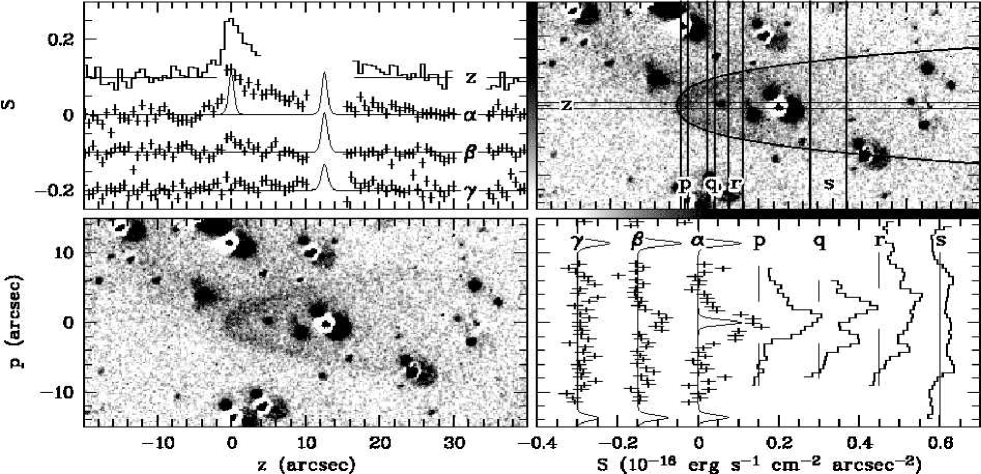
Figure 5: Comparison of the observations with the predicted Balmer emission for an ionisation nebula. As Fig. 3, but with the predicted H$\alpha$ image shown in the top-right panel, and with modelled cross cuts overdrawn. The model reproduces the head of the nebula quite well, but underpredicts the brightness in the tail. This may be because in the tail the assumption of case A for the line emission is inappropriate (Sect. 5.3.4).

In the panels with the fractional abundances in Fig. 4, one sees that these follow the pattern expected from the analytic solution of the structure of the nebula (Eq. 18). Only behind the neutron star there are deviations, due to the expansion of the nebula. The temperature also follows the predictions ahead of the neutron star, but behind it the compression wave caused by the expansion is visible. Due to the expansion, the density is reduced by roughly a factor four far behind the neutron star. The velocities associated with the expansion are predominantly perpendicular to the axis of symmetry, as expected. The maximum radially outward velocity is $6.5{\rm\,km}{\rm\,s^{-1}}$ at $2\times 10^{15}{\rm\,cm}$ behind the neutron star. At large distances, this reduces to $3{\rm\,km}{\rm\,s^{-1}}$ (the reduction is due to cooling; without cooling, the maximum outward velocity is about $10{\rm\,km}{\rm\,s^{-1}}$ and remains this high due to continued photo-ionisation). No shocks form, since the velocity remains well below the sound speed everywhere: $(v/c_{\rm s})_{\rm max}=0.3$.

The predicted H$\alpha$, H$\beta$ and H$\gamma$ fluxes are compared with the observations in Fig. 5. As one can see, the agreement near the head of the nebula is very good, but near the tail the brightness is underpredicted.

5.3.3 Fiddling with the parameters

To see how sensitive our results are to the choice of parameters, we also ran models for different choices, each time allowing ourselves the freedom to adjust $\rho_{\rm ism}$ and $f_{\rm bb}$ such that the match to the observations was as good as possible. We treat the different parameters in turn.

First, we consider the properties of the interstellar medium. If the undisturbed temperature were lower, all temperatures would be somewhat lower and hence the emission less efficient. However, a small change in $f_{\rm bb}$ will compensate for this: for a medium temperature of 100${\rm\,K}$, $f_{\rm bb}=2$ will lead to a model that is hard to distinguish from our base model. The medium may also not be completely neutral, i.e., $\xi_{0}=n_{\rm H^{0}}/n_{\rm H}<1$. This again does not lead to major differences, as long as one chooses a density larger by a factor $\sim\!1/\xi_{0}$, i.e., keeps $n_{\rm H^{0}}$ approximately constant. Even for $\xi_{0}=0.5$, the results are not much different, except that the tail of the nebula becomes slightly narrower because of the “dead mass” that has to be dragged along in the expansion.

Second, we varied the temperature of the neutron star. This will lead to a change in the number of ionising photons as well as a change in their mean energy $\bar{\epsilon}$. We find, however, that we can compensate with a suitable change in $f_{\rm bb}$: one requires $f_{\rm bb}\simeq 2.1$ and 1.4 for temperatures $kT_{\rm ns}=40$ and 60${\rm\,eV}$, respectively. The results look very similar, except that for lower (higher) temperature, the tail is somewhat longer (shorter) and narrower (wider), and the head is very slightly dimmer (brighter). Compensation for the change in brightness requires a change in $\rho_{\rm ism}$ of $\sim\!5\%$.

Third, we considered different inclination. We found that even for inclinations as low as 30°, the main effect is on the width of the tail, which becomes narrower; the length of the tail is hardly affected, while the brightness of the head of the nebula changes only slightly (brighter for lower inclination). The somewhat counter-intuitive result for the width of the tail is a consequence of the fact that the expansion velocity is inversely proportional to $v_{\rm ns}$ (Eq. 29), and, therewith proportional to $\sin i$ (since $v_{\rm ns}=v_{\rm ns,\perp}/\sin i=d\mu_{\rm ns}/\sin i$).

Finally, we considered the distance. For larger distance, less dense interstellar medium suffices to reproduce the brightness of the head, as expected from Eq. 25 (e.g., $\rho_{\rm ism}=5.4\times 10^{-24}{\rm\,g}{\rm\,cm^{-3}}$ for $d=100{\rm\,pc}$). One also finds that the tail of the nebula becomes narrower with increasing distance, as a consequence of the higher space velocity of the neutron star implied by the measured proper motion. Indeed, the width decreases roughly inversely proportional with distance; for $d=100{\rm\,pc}$, it is substantially narrower than observed.

From our attempts, we conclude that the model results are remarkably insensitive to fiddling with the parameters. This is good in the sense that apparently the observed shape of the head of the nebula follows quite naturally from the model, but bad in the sense that, when one matches the brightness of the head, just as naturally one predicts a tail to the nebula that is too faint. We discuss below whether this might be due to one of the assumptions underlying our model being wrong.

5.3.4 Verifying the assumptions

For models that reproduce the brightness of the head of the nebula, the brightness in the tail is lower than observed. Thus, in its present form, the model is incorrect. This may relate to one of the assumptions, which perhaps lead us to overestimate the flux near the head of the nebula, or underestimate the flux in the tail. It may be that we miss an important thermal or emission process, but we argued above that photo-ionisation of Hydrogen and Helium, and collisional excitation and ionisation of Hydrogen dominate all other processes.

The one assumption we have not yet verified, is that of case A for the line emission, i.e., whether the medium is sufficiently optically thin to Lyman lines that, e.g., any Ly$\beta$ line produced by collisional excitation escapes the nebula before being converted in an H$\alpha$ photon (plus two photons in the 2s-1s continuum). With temperatures and densities from our model in hand, we can verify whether case A actually holds.

For the Lyman lines, the line-centre cross-section is given in Eq. 10. At the position of maximum brightness in the nebula, $4.5\times 10^{14}{\rm\,cm}$ ($0\aas@@fstack{\prime\prime}5$) in front of the neutron star, our model has $n_{\rm H^{0}}=1.4{\rm\,cm^{-3}}$ and $T=5.2\times 10^{4}{\rm\,K}$. Thus, over the size of the head of the nebula ($1\arcsec$ or $\sim\!10^{15}{\rm\,cm}$), the line-centre optical depth for Ly$\beta$ photons is $\tau_{\rm Ly\beta,0}=5.8$. Averaged over the Doppler profile, the probability that the photon escapes can be estimated by $p_{\rm esc}\simeq 1.72/(\tau_{0}+1.72)=0.23$ (here, a spherical geometry is assumed; Osterbrock 1989, p. 101). Since every time a Ly$\beta$ photon is absorbed, there is a probability of only $p_{\rm conv,1}=0.118$ that it is converted to H$\alpha$ (instead of being scattered), the total probability that an H$\alpha$ photon is produced is $p_{\rm conv,tot}\simeq p_{\rm conv,1}/(1-(1-p_{\rm conv,1})(1-p_{\rm esc}))=0.37$. This is still substantially smaller than unity and shows that case A at least is a better choice than case B. Some of the photons may still be absorbed close to the head of the nebula, but many may also escape altogether, since in the hot central regions the Doppler profile is substantially broader than in the cooler surroundings. Obviously, for Ly$\gamma$ and Ly$\delta$, the optical depths are lower and hence the case A assumption is better.

The situation is somewhat different, however, in the tail of the nebula, where the neutral Hydrogen density is higher and the temperature lower. For instance, at $z=1.8\times 10^{16}{\rm\,cm}$ (20″ behind the neutron star; slit s), maximum emission is at $p=5.0\times 10^{15}{\rm\,cm}$ ($5\aas@@fstack{\prime\prime}6$ away from the nebular axis), and at this position one has $n_{\rm H^{0}}=2.7{\rm\,cm^{-3}}$ and $T=2.0\times 10^{4}{\rm\,K}$. Over the relevant length scale at this position, $\sim\!3\times 10^{15}{\rm\,cm}$, the optical depth is $\tau_{\rm Ly\beta,0}=54$. Hence, $p_{\rm esc}=0.03$ and $p_{\rm conv,tot}=0.8$.

From the above, we see that case A is not quite appropriate. If one assumes case A, therefore, the emissivities are underestimated, and therewith the required density overestimated. For the head of the nebula, where the gas is hot and highly ionised, the effect will not be very large, but in the tail, where the gas is relatively cool and less ionised, case A is clearly inappropriate. To treat this correctly, one needs to do full radiation transport, which is beyond the scope of the present paper. To get an idea of the effect, however, we can make the opposite assumption for the tail, namely that the medium is optically thick to Lyman lines everywhere (i.e., case B). For this case, the emission in the tail would be increased by a factor $\sim\!2$, which brings it into much closer agreement with the observations. We intend to pursue this in more detail in a future publication.

One other effect we have ignored so far, is continuum pumping by the ionising source (Ferland 1999), in which neutrals absorb continuum photons at Lyman transitions and emit Balmer, Paschen, and other higher-level lines. For H$\alpha$, we estimate a maximum photon rate of $10^{-6}{\rm\,s^{-1}}{\rm\,cm^{-2}}$ from this process; for this estimate, we calculated the neutron star flux at Ly$\beta$ from the observed optical flux, and assumed that all photons within a thermal line width of 0.1 Å (appropriate for $T=5\times 10^{4}{\rm\,K}$) were absorbed and converted to H$\alpha$ (i.e., case B). Even this maximum rate is well below that produced by collisional excitation near the head of the nebula. For the Helium lines, however, continuum pumping will be important, as the nebular emission is due to recombination and therefore very weak. Given the rather large size of the region in which Helium is ionised, however, the emission will be rather diffuse, and hence it is no surprise we do not detect it.

5.3.5 Model inferences

We found that there were two main free parameters in our model, the interstellar medium density $\rho_{\rm ism}$ and the factor $f_{\rm bb}$, which measures the deviation of the spectrum from a black-body. For the density, the value depends on the fraction $\xi_{0}=n_{\rm H^{0}}/n_{\rm H}$; for a distance of 60${\rm\,pc}$, we found that $\rho_{\rm ism}\simeq 7.7\times 10^{-24}\xi_{0}^{-1}{\rm\,g}{\rm\,cm^{-3}}$. Likely, the real value is somewhat lower, since in assuming case A we ignored conversion of Ly$\beta$ to H$\alpha$ photons, which we found was not quite correct. Full radiative transfer calculations are required to infer a more precise value. Pending those, we round down the required Hydrogen number density to $n_{\rm H}\simeq 3\xi_{0}^{-1}{\rm\,cm^{-3}}$.

The factor $f_{\rm bb}$ depends mainly on the neutron-star temperature. This is because these two together set the rate and energy of the ionising photons, the combination of which sets the total energy input, which is well constrained by the size of the nebula. Roughly, one has $E_{\rm in}\propto n_{\rm X}\alpha_{\rm ion}(\bar{\epsilon}-\chi)\propto f_{\rm bb}T^{0.78}$. To keep $E_{\rm in}$ constant, thus requires $f_{\rm bb}\propto T^{-0.78}$. Our model results confirm this expectation; we find that roughly $f_{\rm bb}=1.7T_{50}^{-1}$.

6 Ramifications

RX~J1856.5$-$3754 is the nearest neutron star and the brightest soft X-ray source (in this category; Treves et al. 2000). As such, it is commanding great interest, in particular from spectroscopic X-ray missions. The available data inform us that RX~J1856.5$-$3754 is nearby (60${\rm\,pc}$) and warm (50${\rm\,eV}$), and that possibly it was formed in a nearby stellar association about a million years ago. Beyond this, however, we are very much in the dark about its nature.

The source is puzzling for two reasons in particular. First, using the temperature inferred from the X-ray, ultraviolet and optical energy distribution, the distance derived from the measured parallax and observed flux imply a radius of only $\sim\!7{\rm\,km}$. This is too small for any equation of state (Pons et al. 2001). Second, RX~J1856.5$-$3754 does not show any pulsations. The lack of pulsations in the radio could be due to the beam not intersecting our line-of-sight. The lack of X-ray pulsations (Pons et al. 2001; Burwitz et al. 2001), however, is puzzling, since all well-studied cooling neutron stars do show significant pulsations.

In this paper, we report the discovery of a cometary nebula around RX~J1856.5$-$3754, shining in H$\alpha$ and H$\beta$. We have considered two models to account for the cometary nebula: a pulsar bow shock model and a photo-ionisation model. Both models lead to new, though different, diagnostics that bear upon the origin of this interesting object.

We first summarise the diagnostics below (Sect. 6.1) and then describe what future observational tests could distinguish between the two models (Sect. 6.2). We conclude with a brief discussion about the puzzling absence of pulsations (Sect. 6.3).

6.1 Constraints Provided from Observations of the Nebula

In both models, we can show that the pulsar is moving through a low density medium, $n_{\rm H^{0}}\simeq 0.8{\rm\,cm^{-3}}$ (bow-shock model) or $n_{\rm H^{0}}\simeq 3{\rm\,cm^{-3}}$ (photo-ionisation model). Such densities are typical of the warm neutral medium (WNM) and perhaps even the warm ionised medium (WIM). These two phases of the interstellar medium are expected to pervade about half of interstellar space. Thus, it is not unusual to find RX~J1856.5$-$3754 embedded in one of these.

The two models do not directly constrain the neutral fraction of the ambient gas, $\xi_{0}$. The WNM is expected to be essentially neutral, while for the WIM one finds $\xi_{0}\ga 0.5$ (at least in those few cases where sufficient data exist to allow estimates; see Sect. 4).

Below we discuss additional diagnostics that are peculiar to each of these two models.

6.1.1 Pulsar bow shock

“Balmer-dominated” nebulae have been seen around a few pulsars. The pulsar wind combined with the supersonic motion of the pulsar in an ambient (partially) neutral medium results in a bow shock. The Balmer lines arise from the collisional excitation of ambient neutral atoms as they drift into the post-shock region.

In the framework of the pulsar bow-shock model, RX~J1856.5$-$3754 is a young off-beam pulsar with an energetic pulsar wind powered by rotational energy loss $\dot{E}\simeq 6\times 10^{31}\xi_{0}^{-1}d_{60}^{3}{\rm\,erg}{\rm\,s^{-1}}$. Combining this $\dot{E}$ with the inferred age of $\sim\!10^{6}{\rm\,yr}$, we estimate the spin period ($P$) and the strength of the magnetic dipole field ($B$): $P\simeq 3\chi^{1/2}\xi_{0}^{1/2}{\rm\,s}$ and $B\simeq 10^{13}\chi\xi_{0}^{1/2}{\rm\,G}$; here $\chi=1-(P_{0}/P)^{2}$ with $P_{0}$ being the spin period at birth. Since $\chi\leq 1$ and $\xi_{0}\leq 1$, the estimates are upper limits; they are consistent with values for $P$ and $B$ expected from an ordinary million-year old pulsar.

How secure are these conclusions? At the speed relevant to this source – $100{\rm\,km}{\rm\,s^{-1}}$ – there currently exist no rigorous calculations of Balmer-dominated shocks. In addition, we have not taken into account the pre-ionisation of the ambient gas ahead of the neutron star by the radiation from the neutron star and from the shocked gas, we have not properly modelled the bow shock geometry, and we have ignored issues of radiative transport. Thus, the constraints we derive must be viewed with some caution. With some effort, however, the full modelling effort can be undertaken (J. Raymond, pers. comm.).

6.1.2 Photo ionisation nebula

We also investigated the possibility that the nebular emission is caused by photo-ionisation and heating of the ambient gas by the extreme-ultraviolet radiation of the neutron star. Such nebulae were predicted to exist around rapidly moving, hot neutron stars by Blaes et al. (1995). They should have cometary shape and be rather different from normal ionisation nebulae, in that both recombination and metal-line cooling are irrelevant.

We made analytical estimates which showed that the nebula around RX~J1856.5$-$3754 could indeed be due to photo-ionisation. Since the input atomic physics for the photo-ionisation model is well known and relatively simple, we proceeded by building a detailed model. We find that the model can reproduce the observations in some detail. There are discrepancies as well, but we argued that those could be related to the fact that for the line emission neither case A nor case B is applicable, and hence one has to do full radiative transport.

We concluded that an ionisation nebula could reproduce the observations, provided the ambient density is about $3\xi_{0}^{-1}{\rm\,cm^{-3}}$ and that the extreme-ultraviolet flux (which is responsible for most of the photo-ionisation) is somewhat higher, by a factor $\sim\!1.7$, than expected based on the black-body spectrum that best fits the optical-ultraviolet and X-ray fluxes. Since some deviations of the spectrum from the blackbody distribution are expected, and since deviations are indeed seen at X-ray wavelengths, the required excess at extreme ultra-violet wavelengths does not seem unreasonable. Indeed, in the context of this model, the nebula provides a measurement of the extreme ultraviolet flux, something which is not possible otherwise because of interstellar extinction.

Proceeding further, in the photo-ionisation framework (but not in the bow shock model), it is plausible that the ambient gas will accrete onto the neutron star (if not stopped by a pulsar wind or flung off by a rotating magnetic field). Assuming the Bondi-Hoyle mechanism, we find an accretion radius of $R_{\rm acc}=2GM_{\rm ns}/v_{\rm ns}^{2}=3.7\times 10^{12}d_{60}^{-2}{\rm\,cm}$. This leads to an accretion rate of $\dot{M}=\pi R_{\rm acc}^{2}\rho_{\rm ism}v_{\rm ns}=3\times 10^{9}\,d_{60}^{-3.5}{\rm\,g}{\rm\,s^{-1}}$ (where we used $n_{\rm H}=3d_{60}^{-0.5}{\rm\,cm^{-3}}$ and $X=0.73$). The resulting accretion power is $\sim\!GM_{\rm ns}\dot{M}/R_{\rm ns}\simeq 6\times 10^{29}d_{60}^{-3.5}{\rm\,erg}{\rm\,s^{-1}}$. In contrast, the bolometric luminosity of RX~J1856.5$-$3754 is $\sim\!4\times 10^{31}d_{60}^{2}{\rm\,erg}{\rm\,s^{-1}}$.

Thus accretion, even if takes place, is energetically insignificant. RX~J1856.5$-$3754 is hot not because of accretion. However, accretion will also introduce cosmic composition material to the surface of the neutron star. If the metals settle out rapidly, as is expected for accretion at levels too low to contribute significantly to the luminosity (Brown et al. 1998; Bildsten et al. 1992), this would lead to an atmosphere of almost pure Hydrogen. This would be inconsistent with the observations (Pons et al. 2001; Burwitz et al. 2001).

6.1.3 A combination?

If the nebula is indeed formed by photo-ionisation then any $\dot{E}$ associated with rotational energy loss should be small enough that the standoff radius, $r_{\rm a}$, is less than the observed size of the nebula. Adopting the density required by the ionisation model, $n_{\rm H}\simeq 3{\rm\,cm^{-3}}$, this leads to an upper limit, $\dot{E}\la 2\times 10^{32}d_{60}^{3.5}{\rm\,erg}{\rm\,s^{-1}}$. As before, combining knowledge of $\dot{E}$ with the age of $10^{6}{\rm\,yr}$ inferred from an origin in Upper Scorpius, we derive $P\ga 2\chi^{1/2}{\rm\,s}$ and $B\ga 7\times 10^{12}\chi\,$G. Unfortunately these latter constraints are weak, since $0\leq\chi\leq 1$.

Conversely, if the factor $f_{\rm bb}$ is significantly larger than unity, $f_{\rm bb}\ga 4$, then the bow shock model is ruled out.

6.2 Observational Tests

The critical difference between the pulsar bow shock model and the photo-ionisation model is in the velocity field. In the former, we expect to see more than half (Raymond 1991) of the H$\alpha$ emission to have velocity widths comparable to the shock speed of $100{\rm\,km}{\rm\,s^{-1}}$ both because of the high post-shock temperature and because of large bulk motion. In contrast, in the photo-ionisation model the thermal velocities are moderate, $\la\!40{\rm\,km}{\rm\,s^{-1}}$, and the bulk motion even smaller, $\la\!10{\rm\,km}{\rm\,s^{-1}}$ (see Fig. 4). Thus the simplest test is to obtain higher spectral resolution data. If only narrow lines are seen, then the photo-ionisation model is vindicated. With adequate spatial resolution, one can map the velocity field, for which again the expectations are clearly different in the two models.

A high spatial resolution image of the nebula would be extremely useful. First, independent of which model is correct, such an observation can be used to derive the direction of the velocity vector of RX~J1856.5$-$3754 (because of the intrinsic cylindrical symmetry of both models). Next, it can be used to see whether the nebula is thin with a sharp edge, as expected in the bow shock model, or whether its emission gradually peters out, as expected in the photo-ionisation model. A pulsar wind would evacuate gas up to its stand-off radius and thus the most interesting possible result of a high resolution image would be the discovery of a cavity around RX~J1856.5$-$3754, contained within the nebula. If so, the photo-ionisation model would be vindicated and we would still obtain a direct measure of $\dot{E}$.

6.3 Lack of X-ray Pulsations

From the proper motion, it seems likely that RX~J1856.5$-$3754 originated in the Upper Sco OB association and that it is a a million-year old cooling neutron star. Indeed, for the bow-shock model, the inferred value of an $\dot{E}$ is typical of a million year old pulsar. If so, why does RX~J1856.5$-$3754 not exhibit pulsations? A radio beam might not intersect our line-of-sight, but all well-studied cooling neutron stars show significant pulsations at X-ray wavelengths.

The pulsation in cooling radiation arises because magnetic fields influence the conductivity in the crust and thereby lead to temperature variation at the surface. A hotter thermal component (in addition to any magnetospheric emission) is seen in energetic pulsars and usually attributed to a polar cap heated by pulsar activity.

Among the middle-aged pulsars, we note with interest that the one with the weakest field, PSR B1055$-$52 ($P=197\,$ms, $B\sim 1.1\times 10^{12}\,$G and $\dot{E}\sim 3\times 10^{34}\,$erg s^-1), is also the one whose flux shows weakest modulation, $\la\!10\%$ (Ögelman & Finley 1993). Could it be that RX~J1856.5$-$3754 is a slightly older analogue of PSR B1055$-$52? The pulsed fraction in the cooling emission for RX~J1856.5$-$3754 could be reduced further by appealing to an even weaker magnetic field strength, say to a few $10^{11}\,$G (in the bow-shock picture, this would imply that $\chi\ll 1$, i.e., that the pulsar was born with a period close to the current one). If so, it might have been born with properties like those of the 39.5-ms pulsar PSR B1951+32, which has $B\simeq 5\times 10^{11}{\rm\,G}$ and is associated with the supernova remnant CTB 80 (Kulkarni et al. 1988).

If the suggestion that RX~J1856.5$-$3754 has a magnetic field of a few $10^{11}{\rm\,G}$ is correct, we expect the following: (1) more sensitive observations will reveal pulsations at the level of a few percent; (2) $\dot{E}$, when measured, will be below $2\times 10^{32}{\rm\,erg}{\rm\,s^{-1}}$; (3) at high sensitivity, a weak hot component, $\sim 1\%$ of the total emitted flux, may be identified. All these expectations can be tested with deep Chandra and XMM observations.

Most pulsars that we observe, however, appear to be born with magnetic field strengths upward of $10^{12}{\rm\,G}$. In this respect, the a priori probability seems low that RX~J1856.5$-$3754 has such a weak field. It may be that, after all, RX~J1856.5$-$3754 did not originate in Upper Sco, and is old, lost its magnetic field due to accretion, and perhaps was recently reheated by passing through a dense molecular cloud. Or perhaps RX~J1856.5$-$3754 was just born with a very low magnetic field strength, or lost its field in a binary with a complicated history. These possibilities seem even less plausible. Thus, if our chain of logic, which admittedly is long and has many weak links, is correct, RX~J1856.5$-$3754 is a middle-aged relatively weakly magnetised pulsar whose beam does not intersect our line of sight.

It is ironic that the two brightest nearby neutron stars, RX~J1856.5$-$3754 and RX~J0720.4$-$3125, may well represent the extreme ends of the neutron star magnetic field distribution, one a weak field neutron star and another a magnetar.