A general, three-dimensional fluid dynamics code for stars in binary systems

Abstract

We describe the theory and implementation of a three-dimensional fluid dynamics code which we have developed for calculating the surface geometry and circulation currents in the secondaries of interacting binary systems. The main method is based on an Eulerian-Lagrangian scheme to solve the advective and force terms in Euler’s equation. Surface normalised spherical polar coordinates are used to allow the accurate modelling of the surface of the star, as is necessary when free surfaces and irradiation effects are to be considered. The potential and its gradient are expressed as sums of Legendre polynomials, which allows a very efficient solution of Poisson’s equation. The basic solution scheme, based on operator splitting, is outlined, and standard numerical tests are presented.

1 Introduction

Irradiation of the secondaries in X-ray binaries can dramatically change their appearance and their internal structure. The irradiation pressure force can lead to significant distortions of the surface (Phillips & Podsiadlowski 2002), while irradiation-driven circulation currents can transport significant amounts of energy to the unirradiated side. There is ample observational evidence for the existence of such circulation currents: e.g. in HZ Her/Her X-1 (Kippenhahn & Thomas 1979; Schandl, Meyer-Hofmeister & Meyer 1997), in cataclysmic variables (Davey & Smith 1992), in Nova Sco during outburst (Shahbaz et al. 2000) and in Cyg X-2 (J. Casares & P.A. Charles 1999; private communication), there is clear evidence that a substantial amount of X-ray heated material can move beyond the X-ray horizon. Moreover, persistent residuals in the observed radial-velocity curves in X-ray binaries, e.g. in Nova Sco during outburst (Orosz & Bailyn 1997) and Vela X-1 (Barziv et al. 2001), may provide direct evidence for circulation.

Modelling of the irradiation-induced circulation in binaries is difficult due the three-dimensional nature of the problem. It requires the simultaneous solution of the shape of the irradiated star and the circulation and a proper treatment of the surface boundary conditions.

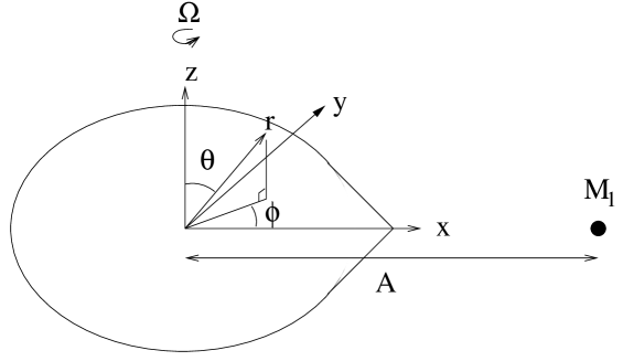
Figure 1: Schematic diagram defining the coordinate systems ($r,~{}\theta,~{}\phi$) and ($x,~{}y,~{}z$) relative to the system geometry and other binary parameters ($A$: orbital separation, $M_{1}$: mass of the primary, ${\mn@boldsymbol{\Omega}}$: angular velocity of the secondary).

Attempts to model circulation in irradiated secondaries have been made by various authors in the past, initially using perturbative methods either in planar geometry (Kippenhahn & Thomas 1979; Kırbıyık & Smith 1976) or spherical geometry (Kırbıyık 1982), and more recently non-perturbatively using smooth-particle hydrodynamics (Martin & Davey 1995). None of these investigations to-date, however, are self-consistent, neither allowing for changes in the surface geometry nor including radiative surface stresses.

On the other hand, circulation currents have been extensively modelled in multi-dimensions in the context of modelling the circulation in the ocean and tidal flows on Earth, where over the years efficient methods have been developed to treat circulation realistically and in a numerically efficient way. A commonly used method is based on an Eulerian-Lagrangian scheme (a description of which may be found in Lu & Wai 1998). This method is similar to the upwind method but more physically sound in the physical treatment of advective terms and has been shown to be unconditionally stable (Casulli 1990; Casulli & Cheng 1992).

The purpose of this paper is to present the philosophy and the details of a fairly general three-dimensional fluid dynamics code which we have specially developed for treating the secondaries in interacting binaries, in particular under the influence of external irradiation. The main method is an application of the Eulerian-Lagrangian method by Lu & Wai (1998) which we have modified for our application, drawing also on the results of related work by Uryū & Eriguchi (1995, 1996, 1998), M$\ddot{\rm{u}}$ller & Steinmetz (1995) and using methods developed in the context of geophysical fluids (see e.g. Pedlosky 1987). At present our code is still somewhat simplified since we do not include the thermodynamic equation, necessitating the use of a polytropic equation of state. In Appendix B, we describe how we plan to generalize the code in the future. In a subsequent paper, we will apply the code first to rotation in the standard Roche problems, and then to study irradiation-driven flows in X-ray binaries, considering both the effects of heating and external radiation pressure, and of radiative surface stresses.

The outline of the paper is as follows. In Section 2 we describe the transformations and the usefulness of surface fitting coordinates, Section 3 describes the basic equations and the dimensionless variables used. The theory and implementation of the calculation of the gradient of the gravitational potential is given in Section 4, including estimates of its accuracy. The general solution method is described in Section 5. Finally, Sections 6 and 7 present standard numerical tests of the code, advection tests and Maclaurin spheroids.

2 Coordinate system

Figure 1 defines the adopted coordinate system, standard spherical polar coordinates centered on the center of mass of the secondary, where the directions of the axes are given by the unit vectors (${\mn@boldsymbol{\hat{r}}},~{}{\mn@boldsymbol{\hat{\theta}}},~{}{\mn@boldsymbol{\hat{\phi}}}$).

2.1 Surface normalised coordinates

For our main applications it is important to model the stellar surface accurately and to allow it to adjust freely to satisfy whatever surface boundary conditions are applied. If the outer edge of the coordinate grid did not coincide with the surface, it would be non-trivial to calculate surface stresses and derivatives along the surface accurately. These difficulties can be avoided by using a grid whose boundary is defined by the stellar surface. To achieve this, we follow Ury$\bar{\rm{u}}$ & Eriguchi (1996) and transform our basic equations (see Section 3) using spherical surface fitting coordinates, i.e.

$$r^{*}=\frac{r}{R(\theta,\phi)}~{},\quad\theta^{*}=\theta~{},\quad\phi^{*}=\phi~{},$$ (1)

where $R(\theta,\phi)$ is the radius of the star in the direction $(\theta,~{}\phi)$. With this definition, $r^{*}$ is restricted to the range

$$0\leq r^{*}\leq 1~{}.$$ (2)

This means that the grid has to adapt continually as the stellar surface changes and that derivatives are transformed according to:

$$R(\theta,\phi)\rightarrow R(\theta^{*},\phi^{*})~{},$$ (3)

$$\frac{\partial{}}{\partial{r}}\rightarrow\frac{1}{R(\theta,\phi)}\frac{\partial{}}{\partial{r^{*}}}~{},$$ (4)

$$\frac{\partial{}}{\partial{\theta}}\rightarrow\frac{\partial{}}{\partial{\theta^{*}}}-\frac{r^{*}}{R(\theta^{*},\phi^{*})}\frac{\partial{R(\theta^{*},\phi^{*})}}{\partial{\theta^{*}}}\frac{\partial{}}{\partial{r^{*}}}~{},$$ (5)

$$\frac{\partial{}}{\partial{\phi}}\rightarrow\frac{\partial{}}{\partial{\phi^{*}}}-\frac{r^{*}}{R(\theta^{*},\phi^{*})}\frac{\partial{R(\theta^{*},\phi^{*})}}{\partial{\phi^{*}}}\frac{\partial{}}{\partial{r^{*}}}~{}.$$ (6)

The surface derivatives $\frac{\partial{R}}{\partial{\theta^{*}}}$ and $\frac{\partial{R}}{\partial{\phi^{*}}}$ are calculated using the potential as described in Appendix C.3.

2.2 Coordinate grid

To define the coordinate grid, we split the star into equally spaced intervals in $r,~{}\cos\theta$ and $\phi$ with a total of $N_{\rm{r}},~{}N_{\theta},~{}N_{\phi}$ elements. The equal spacing in $\cos\theta$ ensures that all grid cells have the same volume. The centers of the grid cells in the $\theta$ and $\phi$ directions are defined by

$$\cos\theta_{\rm{j}}=1-\frac{(j-0.5)}{N_{\theta}}~{},\quad\phi_{\rm{k}}=\frac{2\pi(k-1)}{N_{\phi}}~{},$$ (7)

where we restricted the $\theta$ range assuming even symmetry with respect to the xy-plane, and the surface normalised radial coordinate becomes

$$r_{\rm{i,j,k}}=\frac{(i-0.5)R(\theta_{\rm{j}},\phi_{\rm{k}})}{N_{\rm{r}}}~{},\quad r^{*}_{\rm{i,j,k}}=\frac{i-0.5}{N_{\rm{r}}}~{}.$$ (8)

Velocities are calculated on cell boundaries whilst pressures and densities are evaluated at the centres of cells. Figure 2 shows a cross-section of the grid indicating where various quantities are evaluated.

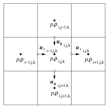
Figure 2: Cross-section of the adopted coordinate grid in the $r$ and $\theta$ directions, indicating where quantities (velocities, $u$, pressure, $p$, and density, $\rho$, are evaluated.

This grid spacing acts so that the entire grid adapts when the surface changes. We adapt this so that if desired the central grid region stays fixed at its initial position when the surface adjusts. This enables us to fix the innermost regions of the grid in situations when we are only interested in the outermost layers. For this purpose we define $N_{\rm c}$ as the number of radial layers from the center whose positions are kept fixed.

$$r_{\rm{i,j,k}}=\left\{\begin{array}[]{ll}\frac{(i-0.5)R_{\rm in}(\theta_{\rm{j}},\phi_{\rm{k}})}{N_{\rm{r}}}&\quad{\rm if}~{}i\leq N_{\rm{c}}~{},\\ \rule{0.0pt}{15.0pt}\frac{N_{\rm c}R_{\rm in}(\theta_{\rm{j}},\phi_{\rm{k}})}{N_{\rm{r}}}+\frac{(i-0.5-N_{\rm c})}{(N_{\rm{r}}-N_{\rm c})}\times\\ \hfill\rule{0.0pt}{12.0pt}\left[R(\theta_{\rm{j}},\phi_{\rm{k}})-\frac{N_{\rm c}R_{\rm in}(\theta_{\rm{j}},\phi_{\rm{k}})}{N_{\rm{r}}}\right]&\quad{\rm otherwise}~{}.\end{array}\right.\hfill$$ (12)

If desired it is possible to redefine the radial spacing so that it is no longer linear but concentrated in a particular region, e.g. near the surface. The number of grid points, however, is kept fixed during a calculation. Fixing the innermost region of the grid also requires an alteration to equations (3–6), since the term proportional to the surface curvature has to be replaced by a term representing the curvature of the grid at the required radius.

$$r^{*}\frac{\partial{R}}{\partial{\theta}}\rightarrow\left\{\begin{array}[]{ll}r^{*}\frac{\partial{R_{\rm in}}}{\partial{\theta}}&\quad{\rm if}~{}i\leq N_{\rm c}~{},\\ \rule{0.0pt}{15.0pt}\frac{N_{\rm c}}{N_{\rm r}}\frac{\partial{R_{\rm in}}}{\partial{\theta}}+\frac{i-0.5-N_{\rm c}}{N_{\rm r}-N_{\rm c}}\times\\ \hfill\rule{0.0pt}{12.0pt}\left(\frac{\partial{R}}{\partial{\theta}}-\frac{\partial{R_{\rm in}}}{\partial{\theta}}\right)&\quad{\rm otherwise}~{}.\end{array}\right.\hfill$$ (16)

3 Basic Equations

The equation of motion relating velocity (${\mn@boldsymbol{u}}$), pressure ($p$), density ($\rho$), frictional force (${\mn@boldsymbol{\mathcal{F}}}$) and potential ($\Phi^{\prime}$) in a frame rotating about the centre of mass of the secondary with angular velocity ${\mn@boldsymbol{\Omega}}$ is

$$\frac{d{\mn@boldsymbol{u}}}{dt}+2{\mn@boldsymbol{\Omega}}{\mn@boldsymbol{\times}}{\mn@boldsymbol{u}}=-\frac{1}{\rho}{\mn@boldsymbol{\nabla}}p-{\mn@boldsymbol{\nabla}}\Phi^{\prime}+{\mn@boldsymbol{\mathcal{F}}}~{},$$ (17)

where

$$\frac{d{\mn@boldsymbol{u}}}{dt}=\frac{\partial{{\mn@boldsymbol{u}}}}{\partial{t}}+({\mn@boldsymbol{u}}{\mn@boldsymbol{\cdot}}{\mn@boldsymbol{\nabla}}){\mn@boldsymbol{u}}~{},$$ (18)

and the potential term is given by

$$\Phi^{\prime}=\Phi+\frac{GM_{1}r\sin\theta\cos\phi}{A^{2}}-\frac{({\mn@boldsymbol{\Omega}}{\mn@boldsymbol{\times}}{\mn@boldsymbol{r}})^{2}}{2}-\frac{GM_{1}}{r_{2}}~{},$$ (19)

where the second term represents a coordinate transformation from the centre of rotation to the centre of the secondary. Here $M_{1}$ is the primary mass, $G$ the gravitational constant, $A$ the binary separation, $r_{2}$ is the distance from the primary to the point ($r,\,\theta,\,\phi$), and the potential of the secondary $\Phi$ is given by Poisson’s equation

$$\nabla^{2}\Phi=4\pi\,G\rho~{}.$$ (20)

The continuity equation,

$$\frac{d\rho}{dt}+\rho{\mn@boldsymbol{\nabla}}{\mn@boldsymbol{\cdot}}{\mn@boldsymbol{u}}=0~{},$$ (21)

can be written in integral form, using the divergence theorem, as

$$\frac{\partial{}}{\partial{t}}\int_{V}\rho\,dV+\int_{dV}\rho\,{\mn@boldsymbol{u}}{\mn@boldsymbol{\cdot}}{\mn@boldsymbol{\hat{n}}}\,dS=0~{},$$ (22)

where ${\mn@boldsymbol{\hat{n}}}$ is a unit surface normal vector. These equations need to be solved along with an equation of state, assumed to be a polytropic equation of state at present which relates pressure and density according to

$$p=K\rho^{\left(1+\frac{1}{n}\right)}~{},$$ (23)

where $K$ and $n$ are the polytropic constant and polytropic index, respectively.

3.1 Boundary conditions

To completely specify the mathematical problem, we also need to specify a set of boundary conditions at the centre and the surface. The central boundary conditions are unproblematic and are given by

$${\mn@boldsymbol{u}}=0~{},\quad\frac{\partial{u_{\rm{r}}}}{\partial{r}}=0~{}.$$ (24)

The simplest boundary condition for the surface are the zero-pressure condition and the conservation of the mass of the secondary,

$$p=0~{},\quad M_{2}=\mbox{constant}~{},$$ (25)

or, more realistically, a pressure condition that assumes an atmosphere in hydrostatic equilibrium, i.e.

$$p=\frac{2g}{3\kappa}~{},$$ (26)

where $g$ is the effective surface gravity, and $\kappa$ the photospheric value of the opacity (see e.g. Kippenhahn & Weigert 1994).

In the case of irradiated stars, a special treatment of the surface layer is required since the irradiation flux is deposited in a thin (turbulent) surface layer (of order an atmospheric scale height), which will generally be smaller than our grid size. A separate atmosphere calculation, which includes the effects of heating and irradiation pressure, then determines the pressure across the surface of the star (analogously to the case of normal stars; also see Tout et al. 1989). In addition, the variation of the radiation pressure force causes a surface stress which drives horizontal motion perpendicular to the stress and vertical motion in a thin turbulent boundary layer (an ‘Ekman’ layer), a process known as ‘Ekman’ pumping. This produces a vertical velocity component in regions where the surface stress varies. This process is entirely analogous to the wind-driven circulation in oceanic circulation systems (see chapter 5 of Pedlosky 1987) and can be treated analogously.

3.2 Surface adjustment

At the end of each time step, the surface is adjusted using the current values of the velocity at the free surface. The surface normal is given by

$${{\mn@boldsymbol{\hat{n}}}}={\mn@boldsymbol{\hat{r}}}-\frac{1}{r}\frac{\partial{R}}{\partial{\theta}}{\mn@boldsymbol{\hat{\theta}}}-\frac{1}{r\sin\theta}\frac{\partial{R}}{\partial{\phi}}{\mn@boldsymbol{\hat{\phi}}}~{}.$$ (27)

The dot product of the surface velocity with the surface normal gives the velocity component normal to the surface. Equating this to the component of the surface adjustment in the radial direction ($\delta r$), which is normal to the surface, yields

$$\delta r=\frac{{\mn@boldsymbol{u}}{\mn@boldsymbol{\cdot}}{\mn@boldsymbol{\hat{n}}}}{{\mn@boldsymbol{\hat{n}}}{\mn@boldsymbol{\cdot}}{\mn@boldsymbol{\hat{r}}}}~{}.$$ (28)

This is added to the current value of $r$ at the end of each time step. In order to ensure mass conservation, the density of each $\theta,\phi$ element is scaled by the ratio of the old and new radii cubed

$$\rho\rightarrow\left(\frac{r}{r+\delta r}\right)^{3}\rho~{}.$$ (29)

This ensures that the density decreases as the radius increases, conserving mass in the process. If mass is not conserved instabilities can develop at the surface of the star. For example, consider the case of a contracting star. As mass leaves the inner radial boundary of the surface layer, no mass loss/gain occurs through the upper boundary and so the density in the surface layer drops to zero. The central density is calculated by extrapolating the densities in the central regions of the star. It is only used as a boundary condition in the potential calculation (Section 4). The extrapolation occurs by extrapolating in the radial direction for each $\theta$ and $\phi$ direction before taking the mean of these values.

3.3 Viscosity

Artificial viscosity is often added in numerical simulations to smooth out the flow and to broaden shock fronts. Stone & Norman (1992) in their code ZEUS-2D use an artificial pressure similar to that of von Neumann & Richtmyer (1950):

$$q=\left\{\begin{array}[]{ll}C^{2}\rho(\Delta v)^{2}&\quad{\rm if}~{}(\Delta v)<0~{},\\ 0&\quad{\rm otherwise}~{},\end{array}\right.$$ (32)

where $\Delta v$ is the change in velocity across a cell and $C=l/\Delta\rm{x}$. $C$ measures the number of zones over which the artificial viscosity spreads a shock and is typically chosen to be $C\sim 3$. This has been generalised to multidimensions by Tscharnuter & Winkler (1979) using an artificial viscous pressure tensor (Q)

$${\bf\sf Q}=\left\{\begin{array}[]{ll}l^{2}\rho{\mn@boldsymbol{\nabla}}{\mn@boldsymbol{\cdot}}{\mn@boldsymbol{u}}\left[{\bf\sf\nabla u}-\frac{1}{3}({\mn@boldsymbol{\nabla}}{\mn@boldsymbol{\cdot}}{\mn@boldsymbol{u}}){\bf\sf e}\right]&\quad{\rm if}~{}{\mn@boldsymbol{\nabla}}{\mn@boldsymbol{\cdot}}{\mn@boldsymbol{u}}<0~{},\\ 0&\quad{\rm otherwise}~{},\end{array}\right.$$ (35)

where e is the unity tensor, ${\bf\sf\nabla u}$ is the symmetrized tensor of the velocity field and $l$ is of the order of the local width of the grid. Following Stone & Norman (1992), we neglect the off-diagonal (shear) components of the artificial viscous pressure tensor. The (nonzero) diagonal elements of the grid are

$${\bf\sf Q_{11}}=l^{2}\rho{\mn@boldsymbol{\nabla}}{\mn@boldsymbol{\cdot}}{\mn@boldsymbol{u}}\left[\frac{\partial{u_{r}}}{\partial{r}}-\frac{1}{3}({\mn@boldsymbol{\nabla}}{\mn@boldsymbol{\cdot}}{\mn@boldsymbol{u}})\right]~{},$$ (36)

$${\bf\sf Q_{22}}=l^{2}\rho{\mn@boldsymbol{\nabla}}{\mn@boldsymbol{\cdot}}{\mn@boldsymbol{u}}\left[\frac{1}{r}\frac{\partial{u_{\theta}}}{\partial{\theta}}+\frac{u_{r}}{r}-\frac{1}{3}({\mn@boldsymbol{\nabla}}{\mn@boldsymbol{\cdot}}{\mn@boldsymbol{u}})\right]~{},$$ (37)

$${\bf\sf Q_{33}}=l^{2}\rho{\mn@boldsymbol{\nabla}}{\mn@boldsymbol{\cdot}}{\mn@boldsymbol{u}}\bigg{[}\frac{1}{r\sin\theta}\frac{\partial{u_{\phi}}}{\partial{\phi}}+\frac{u_{r}}{r}+\frac{u_{\theta}}{r}\cot\theta-$$

$$\phantom{empty}\hfill\frac{1}{3}({\mn@boldsymbol{\nabla}}{\mn@boldsymbol{\cdot}}{\mn@boldsymbol{u}})\bigg{]}~{}.~{}$$ (38)

The frictional force in the momentum equation (17) is

$${\mn@boldsymbol{\mathcal{F}}}=-\frac{1}{\rho}{\mn@boldsymbol{\nabla}}{\mn@boldsymbol{\cdot}}{\bf\sf Q}~{},$$ (39)

where

$${\mn@boldsymbol{\hat{r}}}.{\mn@boldsymbol{\mathcal{F}}}=-\frac{1}{\rho}\frac{\partial{\bf\sf Q_{11}}}{\partial{r}}-\frac{3{\bf\sf Q_{11}}}{\rho r}~{},$$

$${\mn@boldsymbol{\hat{\theta}}}.{\mn@boldsymbol{\mathcal{F}}}=-\frac{1}{\rho r}\frac{\partial{\bf\sf Q_{22}}}{\partial{\theta}}-\frac{\left({\bf\sf Q_{11}+2Q_{22}}\right)}{\rho r}\cot\theta~{},$$

$${\mn@boldsymbol{\hat{\phi}}}.{\mn@boldsymbol{\mathcal{F}}}=\frac{1}{\rho r\sin\theta}\frac{\partial{\left({\bf\sf Q_{11}+Q_{22}}\right)}}{\partial{\phi}}~{},$$ (40)

and where we have used the property ${\bf Tr(\sf Q)}=0$ to eliminate ${\bf\sf Q_{33}}$. This source of viscosity may be switched on or off in the code.

Stone & Norman (1992) also consider an artificial linear viscous pressure,

$$q=C_{1}\rho C_{\rm{a}}\Delta v~{},$$ (41)

to damp instabilities in stagnant regions of the flow, where $C_{1}$ is a constant of order unity and $C_{\rm{a}}$ is the adiabatic sound speed. This is calculated separately for each direction and then added, e.g. in the $r$ direction, as

$${\mn@boldsymbol{\hat{r}}}{\mn@boldsymbol{\cdot}}{\mn@boldsymbol{\mathcal{F}}}=-\frac{1}{\rho}\frac{\partial{q_{\rm{r}}}}{\partial{r}}~{}.$$ (42)

In our code we include the linear viscous pressure which may be switched on or off.

3.4 Dimensionless variables

In the code we use dimensionless variables defined as:

$$\tilde{R}=\frac{R}{{R_{\rm{s}}}}~{},\quad\tilde{\rho}=\frac{\rho}{{\rho_{\rm{c}}}}~{},\quad\tilde{{\mn@boldsymbol{\nabla}}}={R_{\rm{s}}}{\mn@boldsymbol{\nabla}}~{},\quad\tilde{p}=\frac{p}{G{\rho_{\rm{c}}}^{2}{R_{\rm{s}}}^{2}}~{},\quad$$

$$\tilde{\Phi}=\frac{\Phi}{G{\rho_{\rm{c}}}{R_{\rm{s}}}^{2}}~{},\quad\tilde{{\mn@boldsymbol{u}}}=\frac{{\mn@boldsymbol{u}}}{{R_{\rm{s}}}\sqrt{G{\rho_{\rm{c}}}}}~{},\quad\tilde{\Omega}=\frac{\Omega}{\sqrt{G{\rho_{\rm{c}}}}}~{},\quad$$

$$\tilde{M}=\frac{M}{{\rho_{\rm{c}}}{R_{\rm{s}}}^{3}}~{},\quad\tilde{L_{\rm{x}}}=\frac{L_{\rm{x}}}{G{R_{\rm{s}}}^{2}c}~{},\quad\tilde{t}=t\sqrt{G{\rho_{\rm{c}}}}~{},\quad$$

$$\tilde{{\mn@boldsymbol{\mathcal{F}}}}=\frac{{{\mn@boldsymbol{\mathcal{F}}}}}{G{\rho_{\rm{c}}}{R_{\rm{s}}}}~{},\quad\tilde{\nu}=\frac{\nu}{{R_{\rm{s}}}^{2}\sqrt{G{\rho_{\rm{c}}}}}~{},\quad\tilde{\kappa}=\kappa{\rho_{\rm{c}}}{R_{\rm{s}}}~{},$$ (43)

where ${R_{\rm{s}}}$ is the solar radius, ${\rho_{\rm{c}}}$ the initial central density and $G$ the gravitational constant. This transforms equations (17), (22) & (23) to:

$$\frac{d\tilde{{\mn@boldsymbol{u}}}}{d\tilde{t}}+2{\mn@boldsymbol{\tilde{\Omega}}}\times{\mn@boldsymbol{\tilde{u}}}=-\frac{1}{\tilde{\rho}}\tilde{{\mn@boldsymbol{\nabla}}}\tilde{p}-\tilde{{\mn@boldsymbol{\nabla}}}\tilde{\Phi^{\prime}}+{\mn@boldsymbol{\tilde{\mathcal{F}}}}~{},$$ (44)

$$\frac{\partial{}}{\partial{\tilde{t}}}\int_{\tilde{V}}\tilde{\rho}\,d\tilde{V}+\int_{d\tilde{V}}\tilde{\rho}\,{\mn@boldsymbol{\tilde{u}}}{\mn@boldsymbol{\cdot}}{\mn@boldsymbol{\hat{n}}}\,d\tilde{S}=0~{},$$ (45)

$$\tilde{p}=\frac{K\tilde{\rho}^{\left(1+\frac{1}{n}\right)}}{G{R_{\rm{s}}}^{2}{\rho_{\rm{c}}}^{\left(1-\frac{1}{n}\right)}}~{}.$$ (46)

4 Potential calculation

4.1 Theory

M$\ddot{\rm{u}}$ller & Steinmetz (1995) developed an efficient algorithm for solving Poisson’s equation which utilizes spherical coordinates and an expansion into spherical harmonics. This results in an algorithm which has a computational cost proportional to $(L+1)^{2}N_{\rm{r}}N_{\theta}N_{\phi}$ where $L$ is the highest order harmonic considered. The general solution of Poisson’s equation in spherical harmonics, $Y^{lm}(\theta,\phi)$ (Morse & Feshbach 1953) can be written as

$$\Phi(r,\theta,\phi)=-G\sum_{l=0}^{\infty}\frac{4\pi}{2l+1}\sum_{m=-l}^{l}Y^{lm}(\theta,\phi)\times$$

$$\phantom{empty}\hfill\left[\frac{1}{r^{l+1}}C^{lm}(r)+r^{l}D^{lm}(r)\right]~{},\$$ (47)

where

$$C^{lm}(r)=\int_{4\pi}d\Omega^{\prime}Y^{lm*}(\theta^{\prime},\phi^{\prime})\int_{0}^{r}dr^{\prime}{r^{\prime}}^{l+2}\rho(r^{\prime},\theta^{\prime},\phi^{\prime})~{},$$ (48)

$$D^{lm}(r)=\int_{4\pi}d\Omega^{\prime}Y^{lm*}(\theta^{\prime},\phi^{\prime})\int_{r}^{\infty}dr^{\prime}{r^{\prime}}^{1-l}\rho(r^{\prime},\theta^{\prime},\phi^{\prime})~{},$$ (49)

$$d\Omega^{\prime}=\sin\theta^{\prime}d\theta^{\prime}d\phi^{\prime}~{}.$$ (50)

By differentiating this equation we may obtain analytical formulae for the gradient of the potential in spherical coordinates (as derived in Appendix C.1):

$$\frac{\partial{\Phi(r,\theta,\phi)}}{\partial{r}}=-G\sum_{l=0}^{\infty}\frac{4\pi}{2l+1}\sum_{m=-l}^{l}Y^{lm}(\theta,\phi)\times$$

$$\phantom{empty}\hfill\bigg{[}\frac{-(l+1)}{r^{l+2}}C^{lm}(r)+lr^{l-1}D^{lm}(r)\bigg{]}~{}.~{}$$ (51)

$$\frac{\partial{\Phi(r,\theta,\phi)}}{\partial{\theta}}=-G\sum_{l=0}^{\infty}\frac{4\pi}{2l+1}\sum_{m=-l}^{l}Y^{lm}(\theta,\phi)\times$$

$$\left[\frac{P_{l}^{|m+1|}(\cos\theta)}{P_{l}^{|m|}(\cos\theta)}+\frac{m\cos\theta}{\sin\theta}\right]\left[\frac{1}{r^{l+1}}C^{lm}(r)+r^{l}D^{lm}(r)\right]~{}.\$$ (52)

$$\frac{\partial{\Phi(r,\theta,\phi)}}{\partial{\phi}}=-G\sum_{l=0}^{\infty}\frac{4\pi}{2l+1}\sum_{m=-l}^{l}imY^{lm}(\theta,\phi)\times$$

$$\hfill\left[\frac{1}{r^{l+1}}C^{lm}(r)+r^{l}D^{lm}(r)\right]~{}.~{}$$ (53)

For odd $l+m$, ${P_{l}}^{m}(\cos\theta^{\prime})$ is an odd function in $\theta^{\prime}$. Since the density is an even function w.r.t. $\theta^{\prime}$ (because of the assumed symmetry with respect to the $xy$-plane) $\rho(\theta^{\prime},\phi^{\prime},r^{\prime})\sin\theta^{\prime}{P_{l}}^{m}(\cos\theta^{\prime})$ is an odd function and its integral from $\theta=0$ to $\pi$ in equations (48) & (49) is zero. Hence terms odd in $l+m$ do not contribute to the sum, and we only need to include values of $m$ from 0 to $l$ and double the contribution of the positive $m$ term.

In our code we deal with $\Phi^{\prime}$ rather than $\Phi$,

$$\Phi^{\prime}(r,\theta,\phi)=\Phi(r,\theta,\phi)-$$

$$\hfill\frac{(\Omega r\sin\theta)^{2}}{2}+\frac{GM_{1}r\sin\theta\cos\phi}{A^{2}}-\frac{GM_{1}}{r_{2}}~{}.\$$ (54)

This then yields:

$$\frac{\partial{\Phi^{\prime}}}{\partial{r}}=\frac{\partial{\Phi}}{\partial{r}}-r\Omega^{2}\sin^{2}\theta+$$

$$\hfill\frac{GM_{1}\sin\theta\cos\phi}{A^{2}}+\frac{GM_{1}(r-A\sin\theta\cos\phi)}{(A^{2}+r^{2}-2Ar\sin\theta\cos\phi)^{\frac{3}{2}}}~{},\$$ (55)

$$\frac{\partial{\Phi^{\prime}}}{\partial{\theta}}=\frac{\partial{\Phi}}{\partial{\theta}}-(r\Omega)^{2}\sin\theta\cos\theta+$$

$$\hfill\frac{GM_{1}r\cos\theta\cos\phi}{A^{2}}-\frac{GM_{1}Ar\cos\theta\cos\phi}{(A^{2}+r^{2}-2Ar\sin\theta\cos\phi)^{\frac{3}{2}}}~{},\$$ (56)

$$\frac{\partial{\Phi^{\prime}}}{\partial{\phi}}=\frac{\partial{\Phi}}{\partial{\phi}}-$$

$$\hfill\frac{GM_{1}r\sin\theta\sin\phi}{A^{2}}-\frac{GM_{1}Ar\sin\theta\sin\phi}{(A^{2}+r^{2}-2Ar\sin\theta\cos\phi)^{\frac{3}{2}}}~{}.\$$ (57)

4.2 Accuracy

In Appendix C.2, we describe the implementation of this potential calculation in the code. To test the accuracy of the potential calculation, we compared it to three simple cases in which analytical solutions exist. We also compared it to the ZEUS-2D code (Stone & Norman 1992) for which the same tests have been performed. For the purposes of comparison, we chose their test cases in spherical polar coordinates in which they assumed equatorial symmetry as in our calculations. They do not list the number of grid points they used. Here we used $50^{3}$ grid points. Table 1 shows the comparison in the potential calculation for three cases of a homogeneous sphere, a centrally condensed sphere and a homogeneous ellipsoid.

Object	Max. error in $\frac{\partial{\Phi}}{\partial{r}}$	Max. error in ${\mn@boldsymbol{\nabla}}\Phi$ in ZEUS-2D
Homogeneous Sphere	1.02$\times$10-8%	1.11$\times$10-2%
Centrally Condensed Sphere	6.35$\times$10-2%	9.98$\times$10-2%
Homogeneous Ellipsoid	1.53%	1.86%

Table 1: A comparison of the potential calculation in our code, performed on a three-dimensional grid, to the two-dimensional calculations using the ZEUS-2D code for three simple cases with analytic solutions.

Table 1 shows that our potential calculation is more accurate than that of ZEUS-2D regardless of the density distribution. As our calculation is based on a numerical representaion of the analytical value it is extremely accurate for the simplified case of a homogeneous sphere. The centrally condensed sphere shows the accuracy of the radial integration which is resolution limited. The error in the calculation for the homogeneous ellipsoid is smaller than that of the ZEUS-2D calculation. Indeed, it is only large at the surface – throughout the remainder of the star it remains of similar order as in the calculation for the centrally condensed sphere. We have also calculated the error in the $\theta$ derivative of the potential. We find that this is of similar order to the error in the $r$ direction.

5 Solution method

5.1 Operator splitting of the equation of motion

The equation of motion is solved in two parts using the method of operator splitting or fractional step. With this technique the equation of motion is split into two parts. One representing the advective terms, and another representing the force terms. The advantage of this method is that different numerical techniques may be used to solve the two equations representing physically different processes.

We split equation (17) into two parts, one containing the advective terms, the other the force terms. Once the first part is solved, its solution is used in the second part to find the solution corresponding to the full time step. Representing the time derivative of these equations in finite difference form yields

$$\frac{{\mn@boldsymbol{u}}^{a}-{\mn@boldsymbol{u}}^{t}_{\rm{p}}}{\delta t}+2{\mn@boldsymbol{\Omega}}{\mn@boldsymbol{\times}}{\mn@boldsymbol{u}}^{a}=0~{},$$ (58)

$$\frac{{\mn@boldsymbol{u}}^{t+\delta t}-{\mn@boldsymbol{u}}^{a}}{\delta t}=-\frac{1}{\rho}{\mn@boldsymbol{\nabla}}p-{\mn@boldsymbol{\nabla}}\Phi^{\prime}+{\mn@boldsymbol{\mathcal{F}}}~{},$$ (59)

where we have followed the notation of Lu & Wai (1998), and the subscript p refers to the position of the element of interest in the previous time step. Each part of the equation is solved for a full time step ($\delta t$), and we have used the notation ${\mn@boldsymbol{u}}^{a}$ to indicate the solution for the velocity once the first equation, containing the advective terms, has been solved.

By solving the equations using the velocity of the fluid element from the previous time step, the non-linear term $({\mn@boldsymbol{u}}{\mn@boldsymbol{\cdot}}{\mn@boldsymbol{\nabla}}){\mn@boldsymbol{u}}$ is eliminated from the equations. This means that advective terms in the equations are solved in a Lagrangian frame (for fixed mass elements) rather than an Eulerian frame (with fixed positions) where the remainder of the terms are solved for. Hence this method is known as an Eulerian-Lagrangian method. Figure 3 illustrates how ${\mn@boldsymbol{u}}_{\rm{p}}^{t}$ is calculated. The figure shows a cut away element of the fluid. Using the velocity ${\mn@boldsymbol{u}}^{t}$, we calculate the position of the fluid element at a time step $\delta t$ before the present one. Interpolating the velocity grid yields the velocity ${\mn@boldsymbol{u}}_{\rm{p}}^{t}$ at this position. In actuality, we split the time step into a number of substeps enabling an accurate calculation of the streamlines of the fluid. The substep method consists of finding the velocity at a point a substep away and using this velocity to find the velocity in the next substep. This way curved trajectories may be easily followed.

Figure 3: Diagram showing the path interpolation used for the Eulerian-Lagrangian method.

5.2 Solution of the continuity equation on an adaptive grid

The grid used in the code is adaptive. At the end of each time step, the grid is rescaled so that its boundary represents the surface of the star. Thus, the mass within each cell will change at the end of each time step. To compensate for this in solving the integral form of the continuity equation (equation 22), the surface velocity is calculated at each iteration of the continuity equation and the radial velocities used in the calculation are relative to this

$$u^{\prime}_{r}(\theta,\phi)=u_{r}(\theta,\phi)-\frac{i}{N_{\rm{r}}-N_{\rm c}}u_{r}(\theta,\phi)\big{|}_{\rm{s}}~{},$$ (60)

where the prime indicates the velocity used in the calculation and the subscript s a quantity evaluated at the surface. Dorfi shows in LeVeque et al. (1998) [p. 279] that time centering of the equations results in second order accuracy in $\delta t$. Hence the variables are evaluated at half-odd-integer time steps i.e. when calculating the mass flow through a cell boundary we use ${\mn@boldsymbol{u}}^{t+\frac{\delta t}{2}}$ and $\rho^{t+\frac{\delta t}{2}}$.

5.3 Calculation of the pressure gradient at the surface

The radial velocity needs to be calculated at the surface which would require a ghost point for pressure half a radial grid zone past the surface. Instead we use the surface pressure which is one of the boundary conditions. Thus we evaluate the pressure gradient one quarter of a zone below the surface. However, this still yields an incorrect value for the surface pressure gradient, so that in equilibrium it will not balance the potential gradient causing a spurious surface velocity. To correct for this, we calculate the potential gradient a quarter of a zone below the surface and find that this accurately balances the pressure gradient.

5.4 Iteration procedure

Figure 4 shows the iteration procedure used in the code. After initialization the main loop of the code is entered. The Eulerian-Lagrangian method is used to find the solution of the advective terms. A sub loop is then entered in which the velocities and density are solved. Using the current values of pressure and density, the new values for the velocities are calculated. With these velocities the new densities can be determined. Once these have converged, the end of a time step has been reached and the surface is adjusted to fit the new shape of the star. Overall convergence is then tested until a solution is found which is written to an output file. It is not guaranteed that the iteration procedure will always converge.

Figure 4: A flow chart diagram showing the iteration procedure used in the code

6 Advection tests

To test the advection in our code, we use two simple tests. Both are in spherical geometry and have also been carried out by Stone & Norman (1992) for their code ZEUS-2D to which we compare it.

6.1 Expansion of a homogeneous sphere in a velocity field

The first test is a “relaxation” problem for a pressure-free and gravity-free homogeneous gas with a velocity field proportional to the radius ($u_{\rm{r}}=v_{0}r$). The density will decay exponentially with time as

$$\rho(t)=\rho_{0}e^{-3v_{0}t}~{}.$$ (61)

At $v_{0}t=4$, the density should have decayed by almost six orders of magnitude to $\rho=6.144{\mn@boldsymbol{\times}}10^{-6}\rho_{0}$. In our calculation we use $v_{0}=1,\rho_{0}=1$ and three time steps of $10^{-2},10^{-3}$ and $10^{-4}$. The results are shown in Table 2.

Time step	Density at $t$ = 4	Error in the density at $t$ = 4
$10^{-2}$	6.522${\mn@boldsymbol{\times}}10^{-6}$	6.14%
$10^{-3}$	6.181${\mn@boldsymbol{\times}}10^{-6}$	0.60%
$10^{-4}$	6.148${\mn@boldsymbol{\times}}10^{-6}$	0.06%

Table 2: A comparison of the calculated density to the analytical solution for the expansion of a homogeneous sphere in a velocity field.

At $t=4$ our code is in better agreement than ZEUS-2D (5.60${\mn@boldsymbol{\times}}10^{-6}$, 8.8%) for all the time steps considered, the error in the density being directly proportional to the time step considered. Stone & Norman (1992), however, provide no information on the time step they use, so this cannot be compared further.

6.2 Pressure-free collapse of a sphere under gravity

The second advection test we use is the collapse of a homogeneous, pressure-free sphere under gravity. Hunter (1962) showed that

$$\frac{r}{r_{0}}=\cos^{2}\beta~{},\quad\frac{\rho}{\rho_{0}}=\cos^{-6}\beta~{},$$ (62)

where

$$\beta+\frac{\sin 2\beta}{2}=t\sqrt{\frac{8\pi G\rho_{0}}{3}}~{},$$ (63)

and $r_{0}$ and $\rho_{0}$ are the initial values of the radius and the density, respectively. For $r_{0}=\rho_{0}=G=1$, the free-fall time (the time at which the sphere has collapsed to a point) is 0.543. The test was run at two different time steps ($10^{-3}$ and $10^{-4}$), and the density, radius and the mass were compared to the analytical solution and the results obtained with ZEUS-2D.

Time step	Max. error in density at $t$ = 0.535
$10^{-3}$	5.30%
$10^{-4}$	0.50%

Table 3: A comparison of density calculated in the code to the analytical solution for the collapse of a pressure-free sphere.

Table 3 shows the errors in the calculated density in comparison to the analytical solution. In all cases, the density profile remained flat and the mass constant. This demonstrates the ability of the code to adjust the surface of the star correctly. Figure 5 shows a comparison at time $t$ = 0.535 with the analytical solution for a time step of $10^{-4}$. Note how the grid is only defined within the sphere allowing an accurate representation of the problem with no spurious points exterior to the surface. In the calculation with ZEUS-2D, a number of grid points end up outside the surface – a direct consequence of their use of ghost zones beyond the boundary.

Figure 5: Test simulation for the pressure-free collapse of a homogeneous sphere under gravity. The comparison shows the density as a function of radius at dimensionless time $t$ = 0.535 for a time step of $10^{-4}$. The solid curves represent the analytical solution and the open circles our model results.

7 Comparison to Lai, Rasio & Shapiro

7.1 The compressible Maclaurin sequence

Lai, Rasio & Shapiro (1993, hereafter LRS) calculated a sequence of compressible Maclaurin spheroids based on an energy variational method. LRS calculate universal dimensionless quantities that are functions of the eccentricity of the spheroid only. The eccentricity is defined as

$$e=\sqrt{1-\frac{R_{\rm{pole}}^{2}}{R_{\rm{equator}}^{2}}}~{},$$ (64)

where $R_{\rm{pole}}$ and $R_{\rm{equator}}$ are the radii of the pole and equator respectively. Transforming into the dimensionless units used in our code, their equation (3.27) becomes

$$\hat{\Omega}^{2}\equiv\kappa_{n}(1-n/5)\left(\frac{\tilde{\Omega}^{{}^{2}}{\rho_{\rm{c}}}}{\pi\bar{\rho}}\right)~{},$$

where

$$\bar{\rho}=\frac{M}{4\pi\bar{R}^{3}}~{},$$ (65)

is the mean density and

$$\bar{R}={(R_{\rm{pole}}R_{\rm{equator}}^{2})^{\frac{1}{3}}}~{},$$ (66)

is the mean value of the radius of the star.

For a polytropic system, as the polytropic index, $n$, increases, so does the radius of the polytrope (which is defined as the position where the density drops to zero). For non-zero $n$ only one analytical solution exists which has a finite radius. This is the case $n=1$ and has the solution

$$\omega=\frac{\sin\xi}{\xi}~{},$$ (67)

where

$$\xi=r\sqrt{\frac{4\pi G}{(n+1)K}{\rho_{\rm{c}}}^{1-\frac{1}{n}}}~{},\quad\omega=\left(\frac{\rho}{{\rho_{\rm{c}}}}\right)^{\frac{1}{n}}~{}.$$ (68)

This is one of the values for the polytropic index considered in both the calculations of LRS and Ury$\bar{\rm{u}}$ & Eriguchi (1998). Other values for the polytropic index of interest are $n=1.5,~{}3$. These polytropic indices are reasonable representations for the internal structure of convective and radiative stars, respectively. Table 4 gives the ratio of mean density to central density $(\bar{\rho}/{\rho_{\rm{c}}})$ for various polytropic indices (Kippenhahn & Weigert 1994).

$n$	$\bar{\rho}/{\rho_{\rm{c}}}$
1	3.03963 ${\mn@boldsymbol{\times}}10^{-1}$
1.5	1.66925 ${\mn@boldsymbol{\times}}10^{-1}$
3	1.84561 ${\mn@boldsymbol{\times}}10^{-2}$
5	0.0

Table 4: Values of $\xi$ at the surface of a polytrope and the ratio of mean density to central density for various polytropic indices $n$.

In our tests we considered the case $n=1$. This is the only analytical solution which has a finite radius making it a convenient starting approximation. Our code can also run, however, with approximate solutions appropriate for $n=1.5~{}\&~{}3$ using the method of Liu (1996) to calculate the density distributions. Starting from this analytic solution we have calculated a compressible Maclaurin sequence for comparison, where we use 50 grid zones in the $r$ direction and 48 grid zones in the $\theta$ direction. We increased the value of $\Omega$ in units of 0.1 and used a time step of $\delta\tilde{t}=0.001$ to find a converged solution. We also included a linear artificial viscous pressure to damp out oscillations.

Figure 6 represents a comparison to the calculations of LRS. It shows a plot of the dimensionless angular velocity squared against eccentricity. The figure shows that the code accurately calculates the eccentricity for each value of $\Omega$.

Figure 6: Angular velocity squared against eccentricity of an ellipsoid. The dashed curve represents the results of LRS and the solid curve our results for comparison.

8 Future applications

Our first application of the code will be the standard Roche problems. These have recently been considered by Ury$\bar{\rm{u}}$ & Eriguchi (1998), who assumed irrotational flows. We will apply our code to the same case for comparison and then relax the constraint of irrotation, using realistic surface boundary conditions. The second and main application will be the case of irradiation by X-rays in interacting binaries, where we will study the effects of surface heating, irradiation pressure and surface stresses to obtain self-consistent solutions of the geometry and the circulation system in irradiated systems and compare these results to observed systems where irradiation effects have been identified (e.g. HZ Her/Her X-1, Cyg X-2, Nova Sco, Vela X-1, Sco X-1). At a later stage we will extend the code to more realistic stellar models as outlined in Appendix B.

Appendix A System variables

Following are a list of variables used in this paper and a description of what they represent:

$\frac{d}{dt}$ Lagrangian derivative $\frac{\partial{}}{\partial{t}}$ Eulerian derivative $p$ Pressure $\rho$ Density ${\mn@boldsymbol{\mathcal{F}}}$ Frictional force ${\mn@boldsymbol{u}}$ Velocity in the rotating frame ${\mn@boldsymbol{u}}^{a}$ Velocity after the solution of the advective terms in the equation of motion (section 5.1) $\Omega$ Angular velocity of rotation $\Phi$ Potential $G$ Gravitational constant $g$ Surface gravity $r,~{}\theta,~{}\phi$ Spherical Polar coordinates $A$ Separation of the binary $r_{2}$ Distance from the primary to the point $(r,~{}\theta,~{}\phi)$ $M_{1}$ Mass of the primary $M_{2}$ Mass of the secondary ${\mn@boldsymbol{\hat{n}}}$ Unit surface normal vector ${\mn@boldsymbol{\hat{r}}},~{}{\mn@boldsymbol{\hat{\theta}}},~{}{\mn@boldsymbol{\hat{\phi}}}$ Unit vectors in the spherical coordinate system $K,n$ Constants in the polytropic equation of state (equation 23) ~ Superscript denoting dimensionless variable (section 3.4) $N_{\rm{r}},~{}N_{\theta},~{}N_{\phi}$ Number of $r,~{}\theta,~{}\phi$ elements $N_{\rm c}$ Number of innermost radial zones whose position is kept fixed $\rm{i,j,k}$ Subscripts used to denote $r,~{}\theta,~{}\phi$ elements $\tau$ Local optical depth in the secondary $\kappa$ Local value of the opacity $L_{\rm{x}}$ X-ray luminosity of the compact object $q$ Artificial viscous pressure ${\bf\sf Q}$ Artificial viscous pressure tensor $C_{1}$ Constant of order unity used in the calculation of artificial viscous pressure $C_{\rm{a}}$ The adiabatic speed of sound $\xi,~{}\omega$ Variables in the Lane-Emden equation for a polytrope (section 7) $V$ Volume of the secondary $I$ Moment of inertia of the secondary $J$ Angular momentum of the system $T$ Kinetic energy of the secondary $W$ Potential energy of the secondary ^ Superscript denoting universal dimensionless variable with no dependence on polytropic index (section 7) $\bar{R}$ Mean radius of the secondary $R_{\rm{pole}}$ Polar radius of an ellipsoid $R_{\rm{equator}}$ Equatorial radius of an ellipsoid $R_{0}$ Radius of a spherical polytrope of mass equal to the secondary

Appendix B Generalisation to a non-polytrope

In this appendix we describe how the computer code may be extended to more realistic stellar models. The most important change is to use a realistic (non-polytropic) equation of state and the addition of an energy equation, the thermodynamic equation (Tassoul 1978):

$$\rho\frac{dU}{dt}+p{\mn@boldsymbol{\nabla}}{\mn@boldsymbol{\cdot}}{\mn@boldsymbol{u}}=\Phi_{\nu}+\rho\epsilon_{\rm{nuc}}-{\mn@boldsymbol{\nabla}}{\mn@boldsymbol{\cdot}}({\mn@boldsymbol{F}}+{\mn@boldsymbol{F_{\rm{r}}}})~{},$$ (69)

where $U$ is the total internal energy per unit mass, $\Phi_{\nu}$ the heat generation by viscous friction, $\epsilon_{\rm{nuc}}$ the rate of energy released by thermonuclear reactions per unit mass, ${\mn@boldsymbol{F}}$ the heat flux,

$${\mn@boldsymbol{F}}=-\chi{\mn@boldsymbol{\nabla}}T~{},$$ (70)

and ${\mn@boldsymbol{F_{\rm{r}}}}$ is the radiative flux,

$${\mn@boldsymbol{F_{\rm{r}}}}=-\frac{4acT^{3}}{3\kappa\rho}{\mn@boldsymbol{\nabla}}T~{},$$ (71)

where $a$ is the radiation constant and $T$ the temperature. The thermodynamic equation may also be written as

$$\rho T\frac{dS}{dt}=\Phi_{\nu}+\rho\epsilon_{\rm{nuc}}-{\mn@boldsymbol{\nabla}}{\mn@boldsymbol{\cdot}}({\mn@boldsymbol{F}}+{\mn@boldsymbol{F_{\rm{r}}}})~{},$$ (72)

where $S$ is the entropy per unit mass. Landau & Lifshitz (1987) show that

$$\frac{\partial{S}}{\partial{t}}=\left(\frac{\partial{S}}{\partial{t}}\right)_{p}\frac{\partial{T}}{\partial{t}},\quad{\mn@boldsymbol{\nabla}}S=\left(\frac{\partial{S}}{\partial{t}}\right)_{p}{\mn@boldsymbol{\nabla}}T~{}.$$ (73)

Therefore,

$$T\frac{dS}{dt}=c_{\rm{p}}\frac{dT}{dt}~{},$$ (74)

where $c_{\rm{p}}$ is the specific heat at constant pressure. This yields

$$\rho c_{\rm{p}}\frac{dT}{dt}=\Phi_{\nu}+\rho\epsilon_{\rm{nuc}}-{\mn@boldsymbol{\nabla}}{\mn@boldsymbol{\cdot}}({\mn@boldsymbol{F}}+{\mn@boldsymbol{F_{\rm{r}}}})~{}.$$ (75)

To relate pressure, density and temperature, we need an equation of state for the fluid, the simplest of which is given by the ideal gas law,

$$p=\frac{k_{\rm{B}}}{\mu m_{\rm{H}}}\rho T~{},$$ (76)

where $k_{\rm{B}}$ is Boltzmann’s constant, $\mu$ the mean molecular weight and $m_{\rm{H}}$ the mass of the hydrogen atom.

The energy generation rate per unit mass, and the opacity are often represented as power laws of temperature and density (Ury$\bar{\rm{u}}$ & Eriguchi 1995), i.e.

$$\epsilon_{\rm{nuc}}=\epsilon_{0}\rho^{\gamma}T^{\delta}~{},$$ (77)

$$\kappa=\kappa_{0}\rho^{\alpha}T^{-\beta}~{},$$ (78)

where $\epsilon_{0}$, $\gamma$, $\delta$, $\kappa_{0}$, $\alpha$ and $\beta$ are constants. For simplified models for lower main-sequence stars, appropriate values for these constants are

$$\gamma\simeq 1~{},\quad\delta\simeq 4.5~{},$$ (79)

and for Kramers’ opacity law,

$$\alpha=1~{},\quad\beta=3.5~{}.$$ (80)

Inclusion of the thermodynamic equation introduces temperature as another variable into the problem along with other variables which depend on $p,\rho,{\mn@boldsymbol{u}}$ and $T$. This leads altogether to six equations and six unknowns. It also requires an additional surface boundary condition, which can be determined from an atmosphere calculation where the effects of external irradiation (if present) may also be included, just as in the case for standard stellar-structure calculations (e.g. Kippenhahn, Weigert & Hofmeister 1967). These equations have to be solved simultaneously to yield the solution at each time step.

Appendix C The calculation of the potential

In this appendix we derive analytical formulae for the derivatives of the gradient of the potential and describe the technique used in their implementation.

C.1 The derivatives of the potential

Differentiating equations (47) to (49) with respect to $r$, we obtain:

$$\frac{\partial{\Phi(r,\theta,\phi)}}{\partial{r}}=-G\sum_{l=0}^{\infty}\frac{4\pi}{2l+1}\sum_{m=-l}^{l}Y^{lm}(\theta,\phi)\bigg{[}\frac{-(l+1)}{r^{l+2}}C^{lm}(r)+\frac{1}{r^{l+1}}\frac{\partial{C^{lm}(r)}}{\partial{r}}+lr^{l-1}D^{lm}(r)+r^{l}\frac{\partial{D^{lm}(r)}}{\partial{r}}\bigg{]}~{}.$$ (81)

$$\frac{\partial{C^{lm}(r)}}{\partial{r}}=r^{l+2}\int_{4\pi}d\Omega^{\prime}Y^{lm*}(\theta^{\prime},\phi^{\prime})\rho(r^{\prime},\theta^{\prime},\phi^{\prime})~{},$$ (82)

$$\frac{\partial{D^{lm}(r)}}{\partial{r}}=-r^{1-l}\int_{4\pi}d\Omega^{\prime}Y^{lm*}(\theta^{\prime},\phi^{\prime})\rho(r^{\prime},\theta^{\prime},\phi^{\prime})~{}.$$ (83)

Hence,

$$\frac{1}{r^{l+1}}\frac{\partial{C^{lm}(r)}}{\partial{r}}+r^{l}\frac{\partial{D^{lm}(r)}}{\partial{r}}=0~{},$$ (84)

and the $r$ derivative of the potential becomes

$$\frac{\partial{\Phi(r,\theta,\phi)}}{\partial{r}}=-G\sum_{l=0}^{\infty}\frac{4\pi}{2l+1}\sum_{m=-l}^{l}Y^{lm}(\theta,\phi)\bigg{[}\frac{-(l+1)}{r^{l+2}}C^{lm}(r)+lr^{l-1}D^{lm}(r)\bigg{]}~{}.$$ (85)

The $\theta$ derivative is given by

$$\frac{\partial{\Phi(r,\theta,\phi)}}{\partial{\theta}}=-G\sum_{l=0}^{\infty}\frac{4\pi}{2l+1}\sum_{m=-l}^{l}\frac{\partial{Y^{lm}(\theta,\phi)}}{\partial{\theta}}\left[\frac{1}{r^{l+1}}C^{lm}(r)+r^{l}D^{lm}(r)\right]~{}.$$ (86)

Using the definition of the spherical harmonics, we find

$$\frac{\partial{\Phi(r,\theta,\phi)}}{\partial{\theta}}=-G\sum_{l=0}^{\infty}\frac{4\pi}{2l+1}\sum_{m=-l}^{l}\frac{Y^{lm}(\theta,\phi)}{P_{l}^{|m|}(\cos\theta)}\frac{d\left[{P_{l}}^{m}(\cos\theta)\right]}{d\theta}\left[\frac{1}{r^{l+1}}C^{lm}(r)+r^{l}D^{lm}(r)\right]~{}.$$ (87)

Using one of the recurrence relations for Legendre polynomials,

$${P_{l}}^{m}(\cos\theta)=(-1)^{m}\sin^{m}\theta\frac{d^{m}\left[P_{l}(\cos\theta)\right]}{d(\cos\theta)^{m}}~{},$$ (88)

we then obtain

$${P_{l}}^{m+1}(\cos\theta) = (-1)^{m+1}\sin^{m+1}\theta\frac{d^{m+1}\left[P_{l}(\cos\theta)\right]}{d(\cos\theta)^{m+1}}~{},$$ (89)

$$= (-1)^{m+1}\sin^{m+1}\theta\left(\frac{-1}{\sin\theta}\right)\frac{d}{d\theta}\left[\frac{{P_{l}}^{m}(\cos\theta)}{(-1)^{m}\sin^{m}\theta}\right]~{},$$

$$= \frac{d\left[{P_{l}}^{m}(\cos\theta)\right]}{d\theta}-{P_{l}}^{m}(\cos\theta)\left(\frac{m\cos\theta\sin^{m-1}\theta}{sin^{m}\theta}\right)~{}.$$

Rearranging these, we get the required relation

$$\frac{d\left[{P_{l}}^{m}(\cos\theta)\right]}{d\theta}={P_{l}}^{m+1}(\cos\theta)+\frac{m\cos\theta}{\sin\theta}{P_{l}}^{m}(\cos\theta)~{}.$$ (90)

When $m=l$, we set ${P_{l}}^{m+1}$ equal to zero. The $\theta$ derivative is then

$$\frac{\partial{\Phi(r,\theta,\phi)}}{\partial{\theta}}=-G\sum_{l=0}^{\infty}\frac{4\pi}{2l+1}\sum_{m=-l}^{l}Y^{lm}(\theta,\phi)\left[\frac{P_{l}^{|m+1|}(\cos\theta)}{P_{l}^{|m|}(\cos\theta)}+\frac{m\cos\theta}{\sin\theta}\right]\left[\frac{1}{r^{l+1}}C^{lm}(r)+r^{l}D^{lm}(r)\right]~{}.$$ (91)

Finally, the $\phi$ derivative is simply given by

$$\frac{\partial{\Phi(r,\theta,\phi)}}{\partial{\phi}} = -G\sum_{l=0}^{\infty}\frac{4\pi}{2l+1}\sum_{m=-l}^{l}\frac{\partial{Y^{lm}(\theta,\phi)}}{\partial{\phi}}\left[\frac{1}{r^{l+1}}C^{lm}(r)+r^{l}D^{lm}(r)\right]~{},$$ (92)

$$= -G\sum_{l=0}^{\infty}\frac{4\pi}{2l+1}\sum_{m=-l}^{l}imY^{lm}(\theta,\phi)\left[\frac{1}{r^{l+1}}C^{lm}(r)+r^{l}D^{lm}(r)\right]~{}.$$

C.2 Implementation

To implement the expansion of the potential in spherical harmonics, we follow the technique described in M$\ddot{\rm{u}}$ller & Steinmetz (1995), in which the integrals are split into a sum of integrals over sub-intervals. If we denote the position at which equations (48) & (49) are to be evaluated as $r_{\rm{n}}$, $C^{lm}(r_{\rm{n}})$ as $C^{lm}_{\rm{n}}$, and $D^{lm}(r_{\rm{n}})$ as $D^{lm}_{\rm{n}}$:

$$C^{lm}_{\rm{n}}=\sum_{\rm{j=1}}^{N_{\theta}}\sum_{\rm{k=1}}^{N_{\phi}}\left[\int_{\phi_{\rm{k-1}}}^{\phi_{\rm{k}}}\int_{\theta_{\rm{j-1}}}^{\theta_{\rm{j}}}\sin\theta d\theta d\phi Y^{lm*}(\theta,\phi)\sum_{\rm{i=1}}^{n}\int_{r_{\rm{i-1}}}^{r_{\rm{i}}}drr^{l+2}\rho(r,\theta,\phi)\right]~{},$$ (93)

$$D^{lm}_{\rm{n}}=\sum_{\rm{j=1}}^{N_{\theta}}\sum_{\rm{k=1}}^{N_{\phi}}\left[\int_{\phi_{\rm{k-1}}}^{\phi_{\rm{k}}}\int_{\theta_{\rm{j-1}}}^{\theta_{\rm{j}}}\sin\theta d\theta d\phi Y^{lm*}(\theta,\phi)\sum_{\rm{i=n+1}}^{N_{\rm{r}}}\int_{r_{\rm{i-1}}}^{r_{\rm{i}}}drr^{1-l}\rho(r,\theta,\phi)\right]~{}.$$ (94)

Introducing $A^{lm}_{\rm{i,j,k}}$ and $B^{lm}_{\rm{i,j,k}}$,

$$A^{lm}_{\rm{i,j,k}}=\int_{\phi_{\rm{k-1}}}^{\phi_{\rm{k}}}\int_{\theta_{\rm{j-1}}}^{\theta_{\rm{j}}}\int_{r_{\rm{i-1}}}^{r_{\rm{i}}}\sin\theta d\theta d\phi drr^{l+2}Y^{lm*}(\theta,\phi)\rho(r,\theta,\phi)~{},$$ (95)

$$B^{lm}_{\rm{i,j,k}}=\int_{\phi_{\rm{k-1}}}^{\phi_{\rm{k}}}\int_{\theta_{\rm{j-1}}}^{\theta_{\rm{j}}}\int_{r_{\rm{i-1}}}^{r_{\rm{i}}}\sin\theta d\theta d\phi drr^{1-l}Y^{lm*}(\theta,\phi)\rho(r,\theta,\phi)~{},$$ (96)

we may write

$$C^{lm}_{\rm{n}}=\sum_{\rm{i=1}}^{n}\sum_{\rm{j=1}}^{N_{\theta}}\sum_{\rm{k=1}}^{N_{\phi}}A^{lm}_{\rm{i,j,k}}=C^{lm}_{n-1}+\sum_{\rm{j=1}}^{N_{\theta}}\sum_{\rm{k=1}}^{N_{\phi}}A^{lm}_{\rm{n,j,k}}~{},$$ (97)

$$D^{lm}_{\rm{n}}=\sum_{\rm{i=n+1}}^{N_{\rm{r}}}\sum_{\rm{j=1}}^{N_{\theta}}\sum_{\rm{k=1}}^{N_{\phi}}B^{lm}_{\rm{i,j,k}}=D^{lm}_{n+1}+\sum_{\rm{j=1}}^{N_{\theta}}\sum_{\rm{k=1}}^{N_{\phi}}B^{lm}_{\rm{n+1,j,k}}~{}.$$ (98)

We implement this as

$$A^{lm}_{\rm{i,j,k}}=\delta\phi\int_{\theta_{\rm{j-1}}}^{\theta_{\rm{j}}}\sin\theta Y^{lm*}(\theta,\phi_{\rm{k}})d\theta\int_{r_{\rm{i-1}}}^{r_{\rm{i}}}\rho(r,\theta_{\rm{j}},\phi_{\rm{k}})r^{l+2}dr~{},$$ (99)

$$B^{lm}_{\rm{i,j,k}}=\delta\phi\int_{\theta_{\rm{j-1}}}^{\theta_{\rm{j}}}\sin\theta Y^{lm*}(\theta,\phi_{\rm{k}})d\theta\int_{r_{\rm{i-1}}}^{r_{\rm{i}}}\rho(r,\theta_{\rm{j}},\phi_{\rm{k}})r^{1-l}dr~{}.$$ (100)

For the $\theta$ integration we use a Romberg method. A numerical integration is required due to the large $\theta$ size of the cells near the poles which is a result of the equal spacing in $\cos\theta$. For the radial integration we assume that the density varies linearly with $r$ within each cell

$$\rho(r,\theta_{\rm{j}},\phi_{\rm{k}}) = \rho(r_{\rm{i-1}},\theta_{\rm{j}},\phi_{\rm{k}})+\frac{(r-r_{\rm{i-1}})\delta\rho}{(r_{\rm{i}}-r_{\rm{i-1}})}~{},$$ (101)

$$= \rho_{\rm{i-1,j,k}}+\frac{(r-r_{\rm{i-1}})\delta\rho}{(r_{\rm{i}}-r_{\rm{i-1}})}~{},$$ (102)

where

$$\delta\rho=\rho_{\rm{i,j,k}}-\rho_{\rm{i-1,j,k}}~{}.$$ (103)

Hence

$$A^{lm}_{\rm{i,j,k}}=\delta\phi\int_{\theta_{\rm{j-1}}}^{\theta_{\rm{j}}}\sin\theta d\theta Y^{lm*}(\theta,\phi_{\rm{k}})\left[\left(\rho_{\rm{i-1,j,k}}-\frac{r_{i-1}\delta\rho}{r_{\rm{i}}-r_{\rm{i-1}}}\right)\frac{r^{l+3}}{l+3}+\frac{\delta\rho}{(r_{\rm{i}}-r_{\rm{i-1}})}\frac{r^{l+4}}{l+4}\right]^{r_{\rm{i}}}_{r_{\rm{i}}-1}~{},$$ (104)

$$B^{lm}_{\rm{i,j,k}}=\delta\phi\int_{\theta_{\rm{j-1}}}^{\theta_{\rm{j}}}\sin\theta d\theta Y^{lm*}(\theta,\phi_{\rm{k}})\left\{\begin{array}[]{ll}\left[\left(\rho_{\rm{i-1,j,k}}-\frac{r_{\rm{i-1}}\delta\rho}{r_{\rm{i}}-r_{\rm{i-1}}}\right)\ln r+\frac{\delta\rho}{(r_{\rm{i}}-r_{\rm{i-1}})}\frac{r^{3-l}}{3-l}\right]^{r_{\rm{i}}}_{r_{\rm{i}}-1}&\quad{\rm if}~{}l=2~{},\\ \left[\left(\rho_{\rm{i-1,j,k}}-\frac{r_{\rm{i-1}}\delta\rho}{r_{\rm{i}}-r_{\rm{i-1}}}\right)\frac{r^{2-l}}{2-l}+\frac{\delta\rho}{(r_{\rm{i}}-r_{\rm{i-1}})}\ln r\right]^{r_{\rm{i}}}_{r_{\rm{i}}-1}&\quad{\rm if}~{}l=3~{},\\ \left[\left(\rho_{\rm{i-1,j,k}}-\frac{r_{\rm{i-1}}\delta\rho}{r_{\rm{i}}-r_{\rm{i-1}}}\right)\frac{r^{2-l}}{2-l}+\frac{\delta\rho}{(r_{\rm{i}}-r_{\rm{i-1}})}\frac{r^{3-l}}{3-l}\right]^{r_{\rm{i}}}_{r_{\rm{i}}-1}&\quad{\rm otherwise.}\end{array}\right.\hfill$$ (108)

In our calculations we consider spherical harmonics up to and including the $l=14$ term. This choice follows from the results presented by M$\ddot{\rm{u}}$ller & Steinmetz (1995) who find (as we do) that the inclusion of terms of higher order does not significantly affect the calculation for geometries in which the use of spherical coordinates is appropriate.

C.3 Calculation of the surface derivatives

We use the potential to calculate the surface derivatives by considering an incremental change in the potential $d\Phi$

$$d\Phi=\frac{\partial{\Phi}}{\partial{r}}dr+\frac{\partial{\Phi}}{\partial{\theta}}d\theta+\frac{\partial{\Phi}}{\partial{\phi}}d\phi~{}.$$ (109)

It is simple to show that

$$\frac{\partial{R}}{\partial{\theta}}={\frac{\frac{d\Phi_{\rm{s}}}{d\theta}-\left.\frac{\partial{\Phi}}{\partial{\theta}}\right|_{\rm{R}}}{\left.\frac{\partial{\Phi}}{\partial{r}}\right|_{\rm{R}}}}~{},\quad\frac{\partial{R}}{\partial{\phi}}={\frac{\frac{d\Phi_{\rm{s}}}{d\phi}-\left.\frac{\partial{\Phi}}{\partial{\phi}}\right|_{\rm{R}}}{\left.\frac{\partial{\Phi}}{\partial{r}}\right|_{\rm{R}}}}~{},$$ (110)

where $\Phi_{\rm{s}}$ denotes the surface potential and all terms are evaluated at the surface. When the surface is an equipotential the first term in the numerator is zero.

Appendix D Finite difference form of equations

In this appendix we give the finite difference form for the terms used in equations (17) & (22). As velocities are calculated on cell boundaries, and pressure and density at the center of cells, it is simple to represent the pressure term (from equation 17) in finite difference form as

$$\frac{1}{\rho}\frac{\partial{p}}{\partial{r}}=\frac{2N_{\rm{r}}(p_{\rm{i+1,j,k}}-p_{\rm{i,j,k}})}{{R_{\rm{j,k}}}(\rho_{\rm{i+1,j,k}}+\rho_{\rm{i,j,k}})}~{},$$ (111)

and similarly for the derivatives in the $\theta$ and $\phi$ directions. The Coriolis term in the equation of motion is solved using equation (58). With the notation $u,v,w$ to represent $u_{\rm{r}},u_{\theta},u_{\phi}$ for ease of reading, the three components of equation (58) are

$$\frac{u_{\rm{i,j,k}}^{a}-u_{\rm{p}_{\rm{i,j,k}}}^{t}}{\delta t}=2\Omega w_{\rm{i+\frac{1}{2},j,k+\frac{1}{2}}}^{a}\sin\theta_{j}~{},$$ (112)

$$\frac{v_{\rm{i,j,k}}^{a}-v_{\rm{p}_{\rm{i,j,k}}}^{t}}{\delta t}=2\Omega w_{\rm{i,j-\frac{1}{2},k+\frac{1}{2}}}^{a}\cos\theta_{j-\frac{1}{2}}~{},$$ (113)

$$\frac{w_{\rm{i,j,k}}^{a}-w_{\rm{p}_{\rm{i,j,k}}}^{t}}{\delta t}=-2\Omega\left(u_{\rm{i-\frac{1}{2},j,k-\frac{1}{2}}}^{a}\sin\theta_{j}+v_{\rm{i,j+\frac{1}{2},k-\frac{1}{2}}}^{a}\cos\theta_{j}\right)~{}.$$ (114)

The integral form of the continuity equation (22) in finite difference form is

$$\frac{\rho^{t+\delta t}_{\rm{i,j,k}}-\rho^{t}_{\rm{i,j,k}}}{\delta t}\delta\left(\frac{r^{3}}{3}\right)\delta(-\cos\theta)\delta\phi+\rho^{t+\frac{\delta t}{2}}_{\rm{i+\frac{1}{2},j,k}}\big{(}u_{\rm{i,j,k}}{\mn@boldsymbol{\hat{n}}}{\mn@boldsymbol{\cdot}}{\mn@boldsymbol{\hat{r}}}+v_{\rm{i+\frac{1}{2},j+\frac{1}{2},k}}{\mn@boldsymbol{\hat{n}}}{\mn@boldsymbol{\cdot}}{\mn@boldsymbol{\hat{\theta}}}+w_{\rm{i+\frac{1}{2},j,k+\frac{1}{2}}}{\mn@boldsymbol{\hat{n}}}{\mn@boldsymbol{\cdot}}{\mn@boldsymbol{\hat{\phi}}}\big{)}r_{\rm{i+\frac{1}{2},j,k}}^{2}\delta\phi\delta(-\cos\theta)-$$

$$\phantom{empty}\hfill\rho^{t+\frac{\delta t}{2}}_{\rm{i-\frac{1}{2},j,k}}{\mn@boldsymbol{\times}}\big{(}u_{\rm{i-1,j,k}}{\mn@boldsymbol{\hat{n}}}{\mn@boldsymbol{\cdot}}{\mn@boldsymbol{\hat{r}}}+v_{\rm{i-\frac{1}{2},j+\frac{1}{2},k}}{\mn@boldsymbol{\hat{n}}}{\mn@boldsymbol{\cdot}}{\mn@boldsymbol{\hat{\theta}}}+w_{\rm{i-\frac{1}{2},j,k+\frac{1}{2}}}{\mn@boldsymbol{\hat{n}}}{\mn@boldsymbol{\cdot}}{\mn@boldsymbol{\hat{\phi}}}\big{)}r_{\rm{i-\frac{1}{2},j,k}}^{2}\delta\phi\delta(-\cos\theta)+\rho^{t+\frac{\delta t}{2}}_{\rm{i,j+\frac{1}{2},k}}v_{\rm{i,j+1,k}}\sin\theta_{j+\frac{1}{2}}r_{\rm{i,j+\frac{1}{2},k}}\delta r\delta\phi$$

$$\phantom{empty}\hfill-\rho^{t+\frac{\delta t}{2}}_{\rm{i,j-\frac{1}{2},k}}v_{\rm{i,j,k}}\sin\theta_{j-\frac{1}{2}}r_{\rm{i,j-\frac{1}{2},k}}\delta r\delta\phi+\rho^{t+\frac{\delta t}{2}}_{\rm{i,j,k+\frac{1}{2}}}w_{\rm{i,j,k+1}}r_{\rm{i,j,k+\frac{1}{2}}}\delta r\delta(-\cos\theta)-\rho^{t+\frac{\delta t}{2}}_{\rm{i,j,k-\frac{1}{2}}}w_{\rm{i,j,k}}r_{\rm{i,j,k-\frac{1}{2}}}\delta r\delta(-\cos\theta)=0~{}.\ \$$ (115)

References

- [1] Barziv O., Kaper L., van Kerkwijk M. H., Telting J. H., van Paradijs J., 2001, A&A, submitted (astro-ph/0108237)
- [2] Casulli V., 1990, J. Comp. Phys., 86, 56
- [3] Casulli V., Cheng R. T., 1992, Int. J. Numer. Meth. Fluids, 15, 629
- [4] Davey S., Smith R. C., 1992, MNRAS, 257, 476
- [5] Hunter C., 1962, ApJ, 136, 594
- [6] Kippenhahn R., Thomas H. C., 1979, A&A, 75 281
- [7] Kippenhahn R., Weigert A., Stellar Structure and Evolution, Springer, 1994
- [8] Kippenhahn R., Weigert A., Hofmeister E., 1967 in Alder B., Fernbach S., Rothenberg M., Methods in Computational Physics, Vol. 7, p. 129
- [9] Kırbıyık H., 1982, MNRAS, 200, 907
- [10] Kırbıyık H., Smith R. C., 1976, MNRAS, 176, 103
- [11] Lai D., Rasio F. A., Shapiro S. L., 1993, ApJS, 88, 205
- [12] Landau L. D., Lifshitz E. M., Course of Theoretical Physics, Vol. 6: Fluid Mechanics, Butterworth-Heinemann, 1987
- [13] LeVeque R. J., Mihilas D., Dorfi E. A., Mller E., Computational Methods for Astrophysical Fluid Flow, Springer, 1998
- [14] Liu F. K., 1996, MNRAS, 281, 1197
- [15] Lu Q., Wai O. W. H., 1998, Int. J. Numer. Meth. Fluids, 26, 771
- [16] Martin T. J., Davey S. C., 1995, MNRAS, 275, 31
- [17] Morse P. M., Feshbach H., Methods of Theoretical Physics, McGraw-Hill, 1953
- [18] Mller E., Steinmetz M., 1995, Comp. Phys. Comm., 89, 45
- [19] Orosz J. A., Bailyn C. D., 1997, ApJ, 477, 876
- [20] Pedlosky J., Geophysical Fluid Dynamics, Springer, 1987
- [21] Phillips S. N., 2000, D.Phil. Thesis, Oxford University, unpublished
- [22] Phillips S. N., Podsiadlowski Ph., 2002, MNRAS submitted, (astro-ph/0109304)
- [23] Schandl S., Meyer-Hofmeister E., Meyer F., 1997, A&A, 318, 73
- [24] Shahbaz T., Groot P., Phillips S. N., Casares J., Charles P. A., van Paradijs J., 2000, MNRAS, 314, 747
- [25] Stone J. M., Norman M. L., 1992, ApJS, 80, 753
- [26] Tassoul J.-L., 1978 Theory of Rotating Stars, Princeton
- [27] Tscharnuter W. M., Winkler K.-H., 1979, Comp. Phys. Comm., 18, 171
- [28] Tout C.A., Eggleton P.P., Fabian A.C., Pringle, J.E., 1989, MNRAS, 238, 427
- [29] Ury K., Eriguchi Y., 1995, MNRAS, 277, 1411
- [30] Ury K., Eriguchi Y., 1996, MNRAS, 282, 653
- [31] Ury K., Eriguchi Y., 1998, ApJS, 118, 563
- [32] von Neumann J., Richtmyer R. D., 1950, J. App. Phys., 21, 232