A reconstruction of the initial

conditions of the Universe by

optimal mass transportation

Uriel    Frisch^∗,       Sabino    Matarrese^†, Roya Mohayaee^‡∗ & Andrei Sobolevski^§∗

^∗ CNRS, UMR 6529, Observatoire de la Côte d’Azur,
BP 4229, 06304 Nice Cedex 4, France

^† Dipartimento di Fisica “G. Galilei” and INFN, Sezione

di Padova, via Marzolo 8, 35131-Padova, Italy

^‡ Dipartimento di Fisica, Universitá Degli Studi di

Roma “La Sapienza”, P.le A. Moro 5, 00185-Roma, Italy

^§ Department of Physics, M.V. Lomonossov University

119899-Moscow, Russia

Nature$|$ VOL 417$|$ 16 MAY 2002

Reconstructing the density fluctuations in the early Universe that evolved into the distribution of galaxies we see today is a challenge of modern cosmology [1]. An accurate reconstruction would allow us to test cosmological models by simulating the evolution starting from the reconstructed state and comparing it to the observations. Several reconstruction techniques have been proposed [2, 3, 4, 5, 6, 7, 8, 9], but they all suffer from lack of uniqueness because the velocities of galaxies are usually not known. Here we show that reconstruction can be reduced to a well-determined problem of optimisation, and present a specific algorithm that provides excellent agreement when tested against data from N-body simulations. By applying our algorithm to the new redshift surveys now under way [10], we will be able to recover reliably the properties of the primeval fluctuation field of the local Universe and to determine accurately the peculiar velocities (deviations from the Hubble expansion) and the true positions of many more galaxies than is feasible by any other method.

Starting from the available data on the galaxy distribution, can we trace back in time and map to its initial locations the highly structured distribution of mass in the Universe (Fig. 1)? Here we show that, with a suitable hypothesis, the knowledge of both the present non-uniform distribution of mass and of its primordial quasi-uniform distribution uniquely determines the inverse Lagrangian map, defined as the transformation from present (Eulerian) positions ${\bf x}$ to the respective initial (Lagrangian) positions ${\bf q}$.

We first consider the direct Lagrangian map ${\bf q}\mapsto{\bf x}$, which can be approximately written in terms of a potential as ${\bf x}=\nabla_{\bf q}\Phi({\bf q})$ at those scales where nonlinearity stays moderate[11]. This is supported by numerical N-body simulations showing good agreement with a very simple potential approximation, due to Zel’dovich[12], which assumes that the particles move on straight trajectories. Even better agreement is obtained with a refinement, the second-order Lagrangian perturbation method[13, 14, 15, 16], also known to be potential.

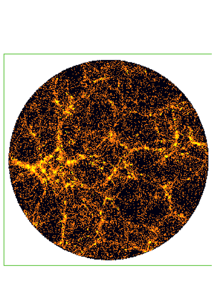
FIG. 1.: $N$-body simulation output (present epoch) used for testing our reconstruction method. In the standard model of structure formation, the distribution of matter in the Universe is believed to have emerged from a very smooth initial state: tiny irregularities of the gravitational potential, which we can still observe as temperature fluctuations of the cosmic microwave background, gave rise to density fluctuations, which grew under their self-gravity, developing a rich and coherent pattern of structures. Most of the mass is in the form of cold dark matter; the luminous matter (galaxies) can be assumed to trace – up to some form of bias – the underlying dark matter. Shown here is a projection onto the $x$-$y$ plane of a 10% slice of the simulation box of size $200h^{-1}$ Mpc. The model, $\Lambda$CDM, uses cold dark matter with cosmological constant and the following parameters: Hubble constant $h=0.65$, density parameters $\Omega_{\Lambda}=0.7$ and $\Omega_{\rm m}=0.3$, normalization factor $\sigma_{8}=0.99$. Points are highlighted in yellow when reconstruction fails by more than $6\,h^{-1}$ Mpc, which happens mostly in high-density regions.

In our “reconstruction hypothesis”, we furthermore assume the convexity of the potential $\Phi({\bf q})$, a consequence of which is the absence of multi-streaming: for almost any Eulerian position, there is a single Lagrangian antecedent. As is well-known, the Zel’dovich approximation leads to caustics and to multi-streaming. This can be overcome in various ways, for example by a modification known as the adhesion model, an equation of viscous pressureless gas dynamics[17, 18]. The latter, which leads to shocks rather than caustics, is known to have a convex potential[19] and to be in better agreement with N-body simulations. Suppression or reduction of multi-streaming requires a mechanism of momentum exchange, such as viscosity, between neighbouring streams having different velocities. This is a common phenomenon in ordinary fluids, such as the flow of air or water in our natural environment. Dark matter is however essentially collisionless and the usual mechanism for generating viscosity (discovered by Maxwell) does not operate, so that a non-collisional mechanism involving a small-scale gravitational instability must be invoked.

Our reconstruction hypothesis implies that the initial positions can be obtained from the present ones by another gradient map: ${\bf q}=\nabla_{{\bf x}}\Theta({\bf x})$, where $\Theta$ is a convex potential related to $\Phi$ by a Legendre–Fenchel transform (see Methods). We denote by $\rho_{0}$ the initial mass density (which can be treated as uniform) and by $\rho({\bf x})$ the final one. Mass conservation implies $\rho_{0}d^{3}q=\rho({\bf x})d^{3}x$. Thus, the ratio of final to initial density is the Jacobian of the inverse Lagrangian map. This can be written as the following Monge–Ampère equation[20] for the unknown potential $\Theta$

$$\hbox{det}\,\left(\nabla_{x_{i}}\nabla_{x_{j}}\Theta({\bf x})\right)=\rho({\bf x})/\rho_{0},$$ (1)

where ‘det’ stands for determinant.

We emphasize that no information about the dynamics of matter other than the reconstruction hypothesis is needed for our method, whose degree of success depends crucially on how well this hypothesis is satisfied. Exact reconstruction is obtained, for example, for the Zel’dovich approximation (before particle trajectories cross) and for adhesion-model dynamics (at arbitrary times).

We note that our Monge–Ampère equation for self-gravitating matter may be viewed as a nonlinear generalisation of a Poisson equation (used for reconstruction in ref. ?), to which it reduces if particles have moved very little from their initial positions.

It has been discovered recently that the map generated by the solution to the Monge-Ampère equation (1) is the (unique) solution to an optimisation problem [21] (see also refs ? and ?). This is the ‘mass transportation’ problem of Monge and Kantorovich [24, 25] in which one seeks the map ${\bf x}\mapsto{\bf q}$ that minimises the quadratic ‘cost’ function

$$I=\int_{\bf q}\rho_{0}|{\bf x}-{\bf q}|^{2}\,d^{3}q=\int_{\bf x}\rho({\bf x})|{\bf x}-{\bf q}|^{2}\,d^{3}x.$$ (2)

Note that ${\bf x}={\bf q}$ is forbidden: as the initial and final density fields $\rho_{0}$ and $\rho({\bf x})$ are prescribed there is a constraint on Jacobian of the map (see Methods).

Next, we take into account that information on the mass distribution is provided in the form of $N$ discrete particles both in simulations and when handling observational data from galaxy surveys. The cost minimisation then becomes what is known in optimisation theory as the assignment problem: find the unique one-to-one pairing of a set of $N$ initial points ${\bf q}_{j}$’s and $N$ final points ${\bf x}_{i}$’s that minimises $I_{\rm discr}=\sum_{i=1}^{N}|{\bf x}_{i}-{\bf q}_{j(i)}|^{2}.$ An immediate consequence is that, for any subset of $k$ pairs of initial and final points ($2\leq k\leq N$), the contribution of these points to the cost function should not decrease under arbitrary permutations of initial points. This property is known to be equivalent to having a Lagrangian map that is the gradient of a convex function [26].

If we restrict ourselves to interchanging just pairs ($k=2$), the map is said to be monotonic, a condition not equivalent to minimisation of the cost function (except in one dimension). In ref. ?, a method of reconstruction called the Path Interchange Zel’dovich Approximation (PIZA) is introduced which uses the same quadratic cost function (obtained by applying a minimum-action argument within the framework of the Zel’dovich approximation). In PIZA, a randomly chosen tentative correspondence between initial and final points is successively improved by swapping pairs of initial particles whenever this decreases the cost function. Eventually, a monotonic map is obtained which usually does not minimise the cost. This explains the non-uniqueness of PIZA reconstruction (also noticed in ref. ?).

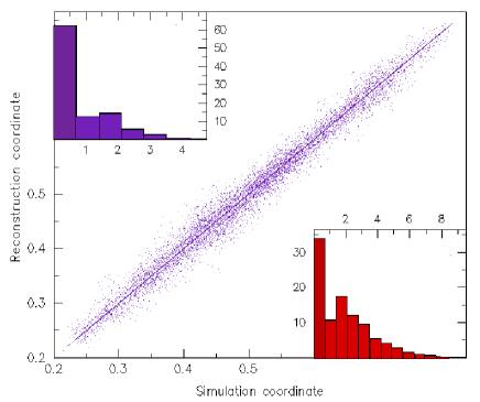
FIG. 2.: Tests of MAK reconstructions of the Lagrangian positions, using the data shown in Fig. 1. The dots near the diagonal are a scatter plot of reconstructed initial points vs. simulation initial points for the coarsest $6.25\,h^{-1}$ Mpc grid with 17,178 points. The scatter diagram uses a ‘quasi-periodic projection’ coordinate $\tilde{q}\equiv(q_{1}+q_{2}\sqrt{2}+q_{3}\sqrt{3})/(1+\sqrt{2}+\sqrt{3})$, which guarantees a one-to-one correspondence between $\tilde{q}$-values and points on the regular Lagrangian grid. The upper left inset is a histogram (by percentage) of distances in reconstruction mesh units between such points; the first slightly darker bin (whose width was taken to be slightly less than one mesh) corresponds to perfect reconstruction (thereby allowing a good determination of the peculiar velocities of galaxies); the lower right inset is a similar histogram for reconstruction on a finer $3.12\,h^{-1}$ Mpc grid using 19,187 points. With the $6.25h^{-1}$ Mpc grid, 62% of the 17,178 points are assigned perfectly and about 75% are within not more than one mesh. With the $3.12h^{-1}$ Mpc grid, we have 34% of exact reconstruction out of 19,187 points. On further refinement of the mesh by a factor two, this degrades to 14%.

There are, however, known deterministic strategies for the assignment problem which give the correct unique solution; their complexity (dependence on $N$ of the number of operations needed) is close to $N^{3}$ for arbitrary cost functions, but can be sharply reduced when the cost function is quadratic. Combining the organisation of data taken from Hénon’s mechanical analogue machine[27] for solving the assignment problem with the dual simplex method of Balinski[28], we have designed an algorithm which gives the optimal assignement for about 20,000 particles in a few hours of CPU on a fast Alpha machine. For historical reasons we call our approach Monge–Ampère–Kantorovich or MAK (see Methods). Details of the algorithms will be given elsewhere; we merely note that, when working with catalogues of several hundred thousands of galaxies expected within a few years, a direct application of the assignment algorithm in its present state could require unreasonable computational resources. A mixed strategy can however be used, in which the assignment problem is solved on a coarse grid while, on smaller scales, the Monge–Ampère equation (1) is solved by a relaxation technique (adapted from ref. ?).

We tested the MAK reconstruction on data obtained by a cosmological $N$-body simulation with $128^{3}$ particles, using the HYDRA code[29] (Fig. 1). Reconstruction was performed on three $32^{3}$ grids with (comoving) meshes given by $\Delta x=6.25\,h^{-1}$ Mpc, $\Delta x/2$ and $\Delta x/4$, where $h$ is the Hubble constant in units of 100 km  s^-1 Mpc^-1. In comoving coordinates, the typical displacement of our mass elements over one Hubble time is about ten $h^{-1}$ Mpc. We discarded those points that, at the end of the simulation (present epoch), were not within a sphere containing about 20,000 points, a number comparable to that of currently available all-sky galaxy redshift catalogues. As the simulation assumes periodic boundary conditions, we also took into account periodicity when calculating the distance between pairs of points. The MAK reconstructions were used to generate a scatter diagram and various histograms allowing comparisons of simulation and reconstructed Lagrangian points (Fig. 2). The results demonstrate the essentially potential character of the Lagrangian map above $\sim 6\,h^{-1}$ Mpc (within the given cosmological model).

We also performed PIZA reconstructions on the coarsest grid and obtained typically 30–40% exactly reconstructed points, but severe non-uniqueness: for two different seeds of the random generator only about half of the exactly reconstructed points were the same.

When reconstructing from observational data, in redshift space (Fig. 3), the galaxies appear displaced radially (as seen by the observer) by an amount proportional to the radial component of the peculiar velocity. We thus performed another reconstruction, with an accordingly modified cost function, that led to somewhat degraded results (Fig. 3) but at the same time provided an approximate determination of peculiar velocities. More accurate determination of peculiar velocities can be done using second-order Lagrangian perturbation theory. The effect of the catalogue selection function can be handled by standard techniques; for instance one can assign each galaxy a ‘mass’ inversely proportional to the catalog selection function [8, 9].

What is the smallest length scale at which an optimisation algorithm such as MAK can be expected to give a unique and reliable reconstruction? The key ingredient here is the simultaneous knowledge of the initial and present mass density fields. MAK-type reconstruction (with a suitable cost based on the equation of a self-gravitating fluid) should therefore be possible down to scales comparable to the thickness of collapsed structures, below which the hydrodynamical description ceases to be meaningful.

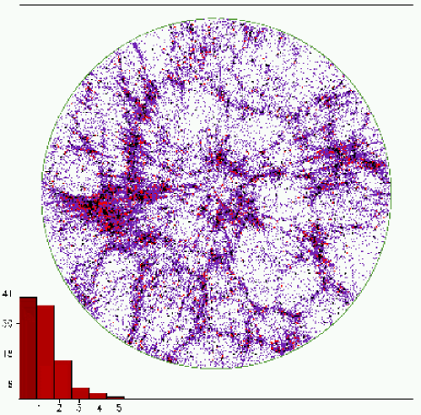
FIG. 3.: Reconstruction test in redshift space with the same data as for the real-space reconstruction tested in the upper left histogram of Fig. 2. The circular redshift map (violet points) corresponds to the same real-space slice as displayed in Fig. 1. The observer is taken to be at the center of the simulation box. Points used for reconstruction within the displayed slice are highlighted in red. Reconstruction is performed by the MAK algorithm with a different cost function, obtained (as in ref. ?) by assuming that the peculiar velocities ${\bf v}$ can be estimated by the Zel’dovich approximation: ${\bm{v}}=f({\bm{{\bf x}}-{\bf q}})$, where $f\approx\Omega_{m}^{0.6}\approx 0.49$. Note that we now have 43% of exactly reconstructed points, included among the 60% which are within not more than $6.25\,h^{-1}$ Mpc from their correct positions.

The fact that MAK guarantees a unique solution and that our present reconstruction hypothesis proved to be very faithful down to $6.5\,h^{-1}\,$Mpc makes our method very promising for the analysis of galaxy redshift surveys[10]. Reconstruction of the primordial positions and velocities of matter will allow us to test the Gaussian nature of the primordial perturbations and the self-consistency of cosmological hypotheses, such as the choice of the global cosmological parameters and the assumed biasing scheme. By obtaining a point-by-point reconstruction of the specific realisation that describes the observed patch of our Universe, we can distinguish between universal properties and the influence of the large-scale environment on the galaxy formation process. Moreover, reconstruction will open a new window not only onto the past but also into the present Universe: it would enable us to make a first-time determination of the peculiar velocities of a very large number of galaxies, using their positions in redshift catalogues.

Methods

Monge–Ampère equation

The Lagrangian map ${\bf q}\mapsto{\bf x}$ is taken to be the gradient of a convex potential $\Phi({\bf q})$; therefore its inverse ${\bf x}\mapsto{\bf q}$ also has a potential representation ${\bf q}=\nabla_{{\bf x}}\Theta({\bf x})$, where $\Theta({\bf x})$ is again a convex function; the two potentials are Legendre–Fenchel transforms of each other (see ref. ?, pp. 61–65):

$$\!\!\Theta({\bf x})=\max_{\bf q}\,\left[{\bf q}\cdot{\bf x}-\Phi({\bf q})\right];\!\!\!\!\quad\Phi({\bf q})=\max_{\bf x}\,\left[{\bf x}\cdot{\bf q}-\Theta({\bf x})\right].$$ (3)

The potential $\Theta$ satisfies the Monge–Ampère equation (1), written for the first time by Ampère[20] by exploiting the property of the Legendre transformation. Note that within the more restricted framework of the Zel’dovich approximation, $\Theta$ differs just by a quadratic additive term from the Eulerian velocity potential[19].

Quadratic cost function

To show that the quadratic cost minimisation leads to the Monge–Ampère equation, we define the displacement field ${\bm{\xi}}({\bf x})\equiv{\bf x}-{\bf q}({\bf x})$ and perform a variation $\delta{\bm{\xi}}({\bf x})$ to obtain, to lowest order, the variation of the cost function $\,\delta I\,=\,\int_{\bf x}2\,{\bm{\xi}}({\bf x})\cdot(\rho({\bf x})\,\delta{\bm{\xi}})\,d^{3}x$. The condition that the Eulerian density remains unchanged, which constrains the variation, is expressed as $\nabla_{\bf x}\cdot(\rho({\bf x})\delta{\bm{\xi}}({\bf x}))=0$. By a simple Lagrange multiplier argument, this implies that ${\bm{\xi}}$ must be a gradient of some function of ${\bf x}$; thus, ${\bf q}={\bf x}-{\bm{\xi}}=\nabla_{\bf x}\Theta({\bf x})$. Furthermore, should $\Theta$ be non-convex and thus lead to multi-streaming, this would prevent the Lagrangian map from being optimal. History of mass transportation Monge[24] posed the following problem: how to optimally move material from one place to another, knowing only its initial and final spatial distributions, the cost being a prescribed function of the distance travelled by ‘molecules’ of material (a linear function in Monge’s original work). Kantorovich[25] showed that Monge’s query was an instance of the linear programming problem and developed for it a theory which found numerous applications in economics and applied mathematics.

Acknowledgements

Special thanks are due to E. Branchini (observational and conceptual aspects), to Y. Brenier (mathematical aspects) and to M. Hénon (algorithmic aspects and the handling of spatial periodicity and of scatter plots). We also thank J. Bec, H. Frisch, B. Gladman, L. Moscardini, A. Noullez, C. Porciani, M. Rees, E. Spiegel, A. Starobinsky and P. Thomas for comments. This work was supported by the BQR program of Observatoire de la Côte d’Azur, by the TMR program of the European Union (UF, RM), by MIUR (SM), by the French Ministry of Education, the McDonnel Foundation, the Russian RFBR and INTAS (AS).