Image and Non-Image Parameters of Atmospheric Cherenkov Events: a comparative study of their $\gamma$-ray/hadron classification potential in UHE regime

Abstract

In this exploratory simulation study, we compare the event-progenitor classification potential of a variety of measurable parameters of atmospheric Cherenkov pulses which are produced by ultra-high energy (UHE) $\gamma$-ray and hadron progenitors and are likely to be recorded by the TACTIC array of atmospheric Cherenkov telescopes. The parameters derived from Cherenkov images include Hillas, fractal and wavelet moments, while those obtained from non-image Cherenkov data consist of pulse profile rise-time and base width and the relative ultraviolet to visible light content of the Cherenkov event. It is shown by a neural-net approach that these parameters, when used in suitable combinations, can bring about a proper segregation of the two event types, even with modest sized data samples of progenitor particles.

1 Introduction

Atmospheric Cherenkov telescopes, being extensively deployed for ground-based $\gamma$-ray astronomy work in the TeV photon energy range for the last 30 years, have invariably to deal with source signals which are extremely weak, both, in absolute terms as also in relation to the background cosmic-ray events (typically $\leq$ 1:100 at photon energies $\geq$ 1 TeV). This has made it mandatory to devise and continually upgrade techniques, in both hardware and software, for optimum acceptance of $\gamma$-ray events and maximal rejection of the background events. A path-breaking advance was made in this direction through the successful implementation of the Cherenkov imaging technique, first attempted by the Whipple collaboration [1]. Here a Cherenkov event is ’imaged’ in the focal-plane of a Cherenkov telescope by recording the two-dimensional distribution of the resulting light pattern with the help of a Cherenkov imaging camera, generally consisting of a square matrix of fast photomultiplier tubes (typical FoV $\sim 3^{\circ}-6^{\circ}$, pixel resolution $\sim 0.15^{\circ}-0.3^{\circ}$). The recorded image, after necessary pre-processing, is parameterised into ’Hillas’ parameters – mainly a set of second-moments which include image shape parameters, called Length (L) and Width (W) and image orientation parameters, like Azwidth (A) and Alpha ($\alpha$) [2]. Both simulation and experimental studies have shown that $\gamma$-ray images are more regular and compact (smaller L and W) as compared with their cosmic-ray counterparts and have a well-defined major axis (orientation) which, in the case of $\gamma$-rays coming from a point $\gamma$-ray source, are oriented closer towards the telescope axis (smaller A and $\alpha$ vis-a-vis randomly oriented cosmic-ray images). Following this approach, the presently operating Cherenkov imaging telescopes, operating in mono or stereo-observation modes, have been able to reject cosmic-ray background events at $\geq 99.5\%$ level, while retaining typically $\sim 50\%$ of the $\gamma$-ray events from a point $\gamma$-ray source and thus register a substantial increase in their sensitivity, compared with non-imaging, generation-I systems.
As a consequence, today, not only do we have for the first time firm detections of at least half a dozen compact $\gamma$-ray sources, but in several cases, their spectra in the TeV energy domain are reasonably well delineated to permit a realistic modeling [3]. Despite this spectacular success of the imaging technique, witnessed during the last one decade, there is still a sense of urgency for seeking a further significant improvement in the sensitivity level in the TeV $\gamma$-ray astronomy field. There are 3 main reasons for this need: One, the detection of fainter compact sources, understandably expected to constitute the major bulk of the TeV source ’catalogue’. Secondly, the detection of $\gamma$-rays from non-compact sources or of a diffuse origin. Only the image shape parameters like L and W, can be used in this case. They are known to be poorer event classifiers compared with the orientation parameter, $\alpha$, in the case of point $\gamma$-rays sources and are found to be grossly inadequate to deal with, for example, the diffuse $\gamma$-ray background of galactic or extragalactic origin. The third motivation for seeking better event-classifier schemes stems from the desirability to use Cherenkov imaging telescopes in a supplementary mode of observations for UHE $\gamma$-ray astronomy and cosmic-ray mass-composition studies in tens of TeV energy range and thereby secure independent information on these important problems through this indirect but effective ground-based [4] technique. Evidently, the required classification schemes in this case will need to have the capability of not only segregating $\gamma$-rays from the general mass of cosmic-ray events, but also to act, at least, as a coarse mass-spectrometer and separate various cosmic-ray elemental groups [5]. Hillas parameters are found to be very good classifiers for smaller images (close to telescope threshold energy) but tend to fail for very large images (higher primary energies of the $\sim$ 10’s TeV) since too many tail pixels are included in the image.
With the above-referred broad aims in mind, serious attempts are presently on to seek enhanced sensitivities and event-characterization capabilities for Cherenkov systems through the deployment of more efficient or versatile image analysis techniques and the inclusion of non-imaging parameters in these classification schemes, for example, rise-time and base-width of the recorded time profile of the atmospheric Cherenkov event or its relative spectral content, i.e. the ultraviolet (U) to visible (V) light flux ratio (U/V ratio). Following in the same spirit, we have recently shown in [5] that fractal parameters can be effectively used to describe Cherenkov images. Thus, it seems meaningful to supplement Hillas parameters with appropriate fractal moments for seeking a better characterization of these images w.r.t. progenitor particle type. In fact, in [5], it has been shown that, by exploiting correlations amongst Hillas parameters with fractal and wavelet moment parameters of Cherenkov images with the help of a properly trained artificial neural network, it is possible not only to efficiently segregate $\gamma$-rays events from the general family of cosmic-ray events but also to separate the latter into low (H-like), medium (Ne-like) and high (Fe-like) mass-number groups with a fairly high quality factor – a job which Hillas parameters alone cannot do as efficiently under similar conditions of net training. Recent work done on this subject by HEGRA [6] group tends to support the above conclusions. The main reasons why this multi-parameter diagnostic approach works is that these parameters look at different aspects of the Cherenkov image: while Hillas parameters are based on its geometrical details, the fractal and wavelet moments are sensitive to image intensity fine-structure and gradients. In this first exploratory exercise, we worked with a large data-base of 24,000 events (consisting of equal numbers of $\gamma$-rays, protons, neon and iron nuclei) and successfully sought their separation by using Hillas, fractal and wavelet-moment parameters. In the present feasibility study, we essentially invert the classification strategy by using an extremely small database (100 events each belonging to $\gamma$-ray, proton, neon and iron parents) and seek their segregation into two main parent species (photons and nuclei) by using a significantly larger parameter-space, consisting of both image (Hillas, fractal and wavelet) and non-image (time-profile and spectral) classifiers.
The present study has a particular relevance for UHE $\gamma$-ray emissions (10’s of TeV) from point sources which are expected to be extremely weak and will need more sensitive signal-retrieval strategies than the one provided by the Hillas image-parameterization scheme alone. The imaging element of the TACTIC array is especially geared for these investigations for it has an unusually large field of view (FoV) of $\sim 6^{\circ}\times 6^{\circ}$ with a uniform pixel resolution of $\sim$ 0.31. It can follow UHE events to larger impact parameter values (400-600 m) and large zenith angle (typically $>40^{\circ}$) and thus expect to detect these events at a significantly higher rate than would be possible for imaging systems with a smaller FoV ($<3^{\circ}$). The related problem of pixel saturation will also not arise generally because most of these UHE events will belong to larger impact parameters (typically $>$ 400 m), where the Cherenkov photon density will be appreciably lesser than what it is expected at smaller zenith angles and smaller extensive air shower (EAS) core distances ($\leq$ 150 m). It is also conceivable that, for at least some $\gamma$-ray sources, the photon spectrum is significantly flatter than what is known for the standard TeV $\gamma$-ray candle source, Crab Nebula (differential photon number exponent $\sim$ 2.7). In such an eventually, one would expect to record a significantly higher flux of UHE photons ($\geq$ 50 TeV) than what follows from a linear extrapolation of the known Crab spectrum in the TeV region. The profound astrophysical implications following an unequivocal detection of an UHE $\gamma$-ray sources $\geq$ 50 TeV) and the unique promise that the TACTIC imaging telescope offers for such an investigation owing to its large FoV and uniform pixel resolution are two factors which have motivated us to carry out the present evaluation exercise.
In this paper, we start with a description of the TACTIC array [7], particularly highlighting the salient features of relevance to the present work. This is followed by a discussion on the methodology adopted for data-base generation for this instrument, using the CORSIKA simulation code [8, 9] and the subsequent derivations of the above-referred image and non-image parameters, after folding in the TACTIC instrumentation details into the simulated data-bases. The results and implications thereof are presented in the next section.

2 TACTIC Array

Experimental details of this instrument, recently commissioned at Mt. Abu ($24.62^{\circ}$ N, $72.75^{\circ}E$, 1257 m asl) in the Western Indian state of Rajasthan have been discussed elsewhere [7, 10]; we present here mainly its salient features as relevant to the present work: TACTIC (for TeV Atmospheric Cherenkov Telescope with Imaging Camera) comprises a compact array of 4 Cherenkov telescope elements, with 1 element (Imaging Element, IE) disposed at the centroid and 3 elements (Vertex Elements, VE) placed at the vertices of an equilateral triangle of 20 m side (Fig. 1). Each telescope element deploys a tessellated light reflector of 9.5 m² mirror area and composed of 34 $\times$ 0.6 m diameter spherical glass mirrors (front-aluminized) of a radius of curvature $\sim$ 8 m. The mirror facets are arranged in a Davis-Cotton geometrical

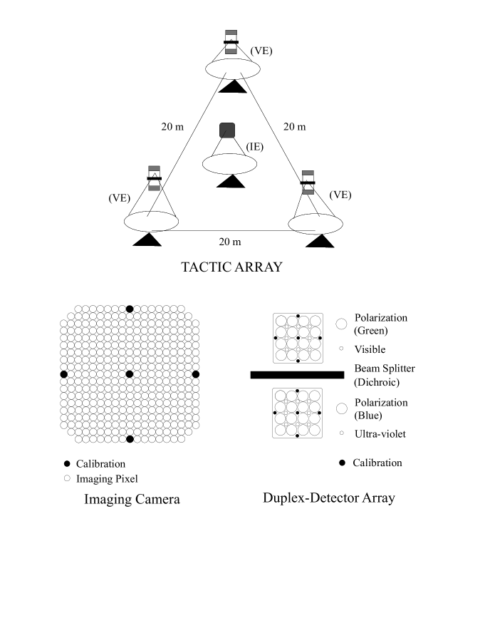
Figure 1: Sketch of the TACTIC array and the cameras for high-sensitivity spectral and temporal investigations on $\gamma$-ray sources in the photon energy range of $\sim 1-100\,$TeV (details see text).

configuration to yield an on-axis spot-size of 0.2 cm diameter. The light reflectors are placed on alt-azimuth mounts and can be synchronously steered with a PC-based drive system with a source-tracking accuracy of $\leq$ 2 arcmin.
The IE of the TACTIC array yields high-definition images of atmospheric Cherenkov events generated by $\gamma$-ray and cosmic ray progenitors with primary energies $\geq$ 1 TeV. For this purpose, this element is provided with a focal-plane imaging camera consisting of 349 fast-photomultiplier pixels (Electron Tubes Ltd., 9083UVB) and arranged in a closely-packed truncated square configuration to yield an FoV $\sim 6^{\circ}\times 6^{\circ}$ with a uniform pixel-resolution of $\sim 0.31^{\circ}$. The focal-plane instrumentation of each VE is designed primarily to record various non-image characteristics of the recorded Cherenkov event, including its linear polarization state, time-profile and ultraviolet-to-visible light spectral content (U/V ratio). For this purpose, as shown in Figure 1, this instrumentation consists of duplex PMT detector (ETL9954 B) arrays which are placed across a 1:1 optical beam splitter, mounted midway between the PMT detector arrays at right angles to the telescope principal axis. There are $16\times 0.91^{\circ}$ diameter PMT detectors in each array which are provided with suitably-oriented sheet-polarizers (near-UV transmitting, Polaroid-make HNB’ type) to measure the linear polarization state of the recorded Cherenkov events. In addition, they are provided with appropriate back-end electronics to record the time-profile of the detected event with $\sim$ 1 ns resolution. The response function of this instrumentation, from PMT onwards, can be approximately represented by a triangular pulse with a rise-time of $\sim$ 2 ns and decay time of $\sim$ 4.5 ns. As is evident from Figure 1, a total of 8 PMT pairs are also provided in the VE focal-plane instrumentation to ’sample’ the relative ultraviolet (U-pixels, $\lambda\sim$ 280-310 nm) to visible (V-pixels, $\lambda\sim$ 310-450 nm) light content of the recorded events. Each U-pixel consists of the PMT type ETL D921 and is placed on the reflection side of the beam-splitter, exactly opposite to its mating V-pixel (ETL 9097B), placed across the beam-splitter (transmission side).
The TACTIC event trigger is based on a memory-based proximity or ‘topological’ trigger-generation scheme which stipulates coincident ‘firing’ of Nearest-Neighbor Non-Collinear Triplet (3 NCT) pixels with a coincidence resolving gate of $\sim$ 20 ns from within the innermost 240 (16 $\times$ 15) pixels of the 349-pixel IE camera [10]. In response to each such trigger, the TACTIC data acquisition system records the photo-electron content of each IE and VE pixel (for image, polarization and U/V spectral information) and the composite time-profile of the Cherenkov event as ’seen’ by all the 32 $\times$ 0.9^∘ dia pixels of the VE camera. All the PMT of the IE and VE can be gain-calibrated in an absolute way, based on a scheme employing the single-photoelectron counting procedure along with radio-active (Am-241) and fluorescent light pulsers.
In the normal (low threshold) mode of operation, deployed on dark, clear nights, the TACTIC follows a putative $\gamma$-ray source across the sky over the zenith-angle range $\theta\leq 40^{\circ}$ and records background cosmic ray events with rates $\leq$ 10 Hz (trigger threshold for $\gamma$-rays, $\sim$ 0.7 TeV) [11]. On the other hand, in the supplementary mode of operation, for UHE $\gamma$-ray astronomy and cosmic ray composition studies in 10’s of TeV energy region and telescope array is planned to be employed, over $\theta$ range $\sim 40-60^{\circ}$. This mode of operation has the advantage of significantly increasing the effective detection area and, in turn, leads to an appreciable enhancement in the relative number of UHE events coming from larger core distances and also not suffering from the problem of image saturation effects.

3 Simulated data-bases

The scheme adopted here for generating TACTIC-compatible data-bases through the CORSIKA simulation code (Version 4.5) [8, 9] using the VENUS code for the hadronic high-energy interactions [12], has been discussed in detail in [5]. In essence, this data-base consists of arrival direction and arrival time of Cherenkov photons, received within a specified wavelength interval by each of the TACTIC mirrors in response to the incidence on the atmosphere of a $\gamma$-ray photon (energy $E_{\gamma}$ = 50 TeV, zenith angle $\theta$ = 40^∘) or a cosmic-ray primary (type: proton, neon or iron nucleus; $E_{h}$ = 100 TeV, $\theta$ = $40^{\circ}\pm 2^{\circ}$). Atmospheric extinction is duly accounted for as a function of the Cherenkov photon wavelength. The received Cherenkov photons are ray-traced into the TACTIC focal-plane instrumentation and converted into equivalent photoelectrons (pe) after folding in the mirror optical characteristics [13], the photocathode spectral response and the beam-splitter wavelength-dependent reflection and transmission coefficients (last one in case of VE only). The 2D-distribution of the number of pe, thus registered by various pixels of the IE camera, constitutes the high-resolution Cherenkov image. Similarly, the pe contents, separately registered by all the U- and V- pixels of a VE camera, yield the U/V spectral ratio of the Cherenkov event, while the ’arrival-time’ distribution of the pe’s, as noted in the image-plane of a VE camera $(32\times 0.9^{\circ}$ dia PMT only), gives the time-profile of this event. The sheet polarizers, normally used with these 32 PMT of the VE camera for polarization measurements, are assumed to be absent for the present simulation exercise. 100 showers each of $\gamma$-rays (50 TeV) and protons, neon and iron nuclei (100 TeV) have been simulated in this manner.
This scheme for data-base generation allows to simultaneously obtain the desired data for the TACTIC array, assumedly placed at various distances (R $\sim$ 10 m - 300 m) from the shower core. We use here the data corresponding to the representative R $\sim$ 195 m, consisting of only 100 Cherenkov images and associated time-profile and U/V data and belonging to each of the 4 primary types considered here. Similar data has been obtained for two other core distances R $\sim$ 245 m and R $\sim$ 295 m.

4 Hillas Parameters

Cherenkov images of $\gamma$-ray showers are mainly elliptical in shape, hence compact. The Cherenkov images of hadronic showers are mostly irregular in shape, implying that gamma rays can be distinguished from hadron events on the basis of shape and compactness of Cherenkov images. The process of $\gamma$/hadron separation needs parameterization and this parameterization was first introduced by Hillas [2]. The resulting Hillas parameters can be generally classified into either ‘shape’ parameters such as Length (L) and Width (W) which characterize the size of the image, or into orientation parameters such as alpha $\alpha$, which is the angle of the image length with the direction of the source location within the field of view of the camera. The azwidth parameter combines both the image shape and orientation features.
We have calculated the following second moments for the simulated Cherenkov images: shape parameters like Length (L), Width (W) and Distance (D) and orientation parameters like alpha ($\alpha$), Azwidth (A), and Miss (M). In so far as the image orientation parameters are concerned, they are found to be small for $\gamma$-rays, assumed here to be coming from a point-source placed along the telescope-axis. For the nuclear progenitors, $\alpha$ (or other orientation parameters) has no significant classification potential, since all these particles are assumed to be randomly oriented around the telescope axis (the same conclusion would hold for $\gamma$-rays of a truly diffuse origin). The average values of some representative Hillas parameters are listed in Table 1 for comparison, where the different hadronic primaries are combined.

Table 1: Average values of Hillas parameters for primary gammas and hadrons. The values of the different hadron species are combined. All values are in angular degrees.

Parameter	Length	Width	Distance	Azwidth	Miss	Alpha
Gamma rays	0.62	0.42	1.0	1.4	0.18	6.4
hadrons	0.71	0.43	1.2	0.56	0.53	32.8

5 Multifractal moments

Employing the prescription given in [5], we have calculated the multifractal moments [14, 15] of the simulated TACTIC images recorded within the innermost 256 pixels of its imaging camera. For this purpose, the image has been divided into $M=2^{\nu}$ equal parts, where $\nu$ =2,4,6 and 8 is the chosen scale-length. The multifractal moments are given as:

$$G_{q}(M)=\Sigma^{M}_{j=1}(\frac{k_{j}}{N})^{q}$$ (1)

where N is the total number of pe in the image, $k_{j}$ is the number of pe in the k^th cell and q is the order of the fractal moment. In case of a fractal, $G_{q}$ shows a power-law behavior with M, i.e.,

$$G_{q}\sim M^{\tau_{q}}$$ (2)

where

$$\tau_{q}=\frac{1}{ln2}\frac{d~{}ln~{}G_{q}}{d\nu}\,\,.$$ (3)

For a fractal structure, there exists a linear relationship between the natural logarithm of $G_{q}$ and $\nu$ and the slope of this line, $\tau_{q}$, is related to the generalized multifractal dimensions, $D_{q}$, by:

$$D_{q}=\frac{\tau_{q}}{q-1},q\neq 1$$ (4)

where -6 $<$ q $<$ 6 is the order the multifractal moment. In [5], we have used 2 multifractal dimensions, $D_{2}$ and $D_{6}$, as classifiers and have achieved a fairly high discrimination power through them for a large composite database of 2,4000 images. On the contrary, since the database size here is significantly smaller (only 100 images for each primary type), it is difficult in this case to clearly identify one (or few) fractal dimensions by the method of overlap of distributions.
By using the correlation ratio we were able to identify $D_{4}$ and $D_{6}$ as having a minimum correlation. A correlation ratio between two variables, say X and Y, is defined as

$$r=\frac{\sum_{i=1}^{n}(X_{i}-\overline{X})(Y_{i}-\overline{Y})}{\sqrt{(\sum_{i=1}^{n}(X_{i}-\overline{X})^{2})(\sum_{i=1}^{n}(Y_{i}-\overline{Y})^{2})}}$$ (5)

The correlation ratio r is a measure of linear association between two variables. A positive coefficient indicates that, as one value increases the other tends to increase whereas a negative coefficient indicates as one variable increases the other tends to decrease. $D_{4}$ and $D_{6}$ are thus relatively independent and should as such provide the best possible segregation of the primary masses.

6 Wavelet Moments

Wavelets can detect both the location and the scale of a structure in an image. These are parameterised by a scale (dilation parameter) ’a’ $>$ 0 and a translation parameter ’b’ (-$\infty<$ b $<\infty$) [17, 18], such that

$$\phi(x)=\frac{\psi(x-b)}{a}\,\,.$$ (6)

Since we are analyzing Cherenkov images which are fractal in nature, it is the dilation parameter ’a’ which is of interest to us here rather than the translation parameter ’b’. The wavelet moment [17] $W_{q}$ is given as :

$$W_{q}(M)=\Sigma^{M}_{j-1}(\frac{|k_{j-1}-k_{j}|}{N})^{q}$$ (7)

where $k_{j}$ is the number of pe in the j^th cell in a particular scale, and $k_{j+1}$, in the j^th cell in the consecutive scale. The wavelet moment has been obtained by dividing the Cherenkov image into M = 4, 16, 64 and 256 equally-sized parts with 64, 16, 4 and 1 PMT pixels respectively and counting the number of pe in each part. The difference of probability in each scale gives the wavelet moment. It turns out that for a Cherenkov image

$$W_{q}\sim M^{\beta_{q}}$$ (8)

implying that the wavelet moment $W_{q}$ bears a power-law relationship with M. As was shown in [5], the exponent $\beta_{q}$ (q = 1-6) is found to be sensitive to the structure of the Cherenkov image and has the lowest value for $\gamma$-rays, followed by protons, neon and iron nuclei, in increasing order of the nuclear charge. In [5] only the wavelet parameters $\beta_{2}$ and $\beta_{6}$ were used for image characterization on account of the fairly large database deployed there. In the present work, we prefer to use the wavelet parameters $\beta_{1}$ and $\beta_{5}$ as classifiers. They have been chosen by the method of minimum correlation.

7 Time parameters

There have been several reports in literature tentatively suggesting a dependence of various time-parameters of Cherenkov pulse-profiles, including their rise-times and base-width on the progenitor type. While most of these suggestions are based on simulation studies [19], there is one piece of experimental work wherein temporal profiles of Cherenkov pulses, recorded by an atmospheric Cherenkov telescope system, have been utilized to preferentially select $\gamma$-ray events from the cosmic-ray background events. Using a largely ad-hoc approach for this selection, this group claimed the detection of a TeV $\gamma$-ray signal from the Crab Nebula in 1.5 hours of observation at 4.35 significance level. The observations were carried out with a 11 m-diameter solar collector-based Cherenkov telescope [20]. More recent simulation investigations [21] have indicated that the differences in the Cherenkov pulse profiles of different primary types are related to the various details of development of EAS initiated by $\gamma$-ray and nuclear-primaries in the atmosphere, including the important role of muon secondaries in the latter case. Thus, the pulse from a $\gamma$-ray primary is expected to have a relatively smooth profile with a typical rise-time of $\sim$ 1 ns, and a decay-time of $\sim$ 2 ns, while the temporal profile of a hadron-origin has relatively longer rise and decay times and, in addition, a superimposed microstructure, possibly due to Cherenkov light produced by single muons, moving close to the detector system.
One of the output parameters in the CORSIKA is the Cherenkov photon arrival time. The measurement of time begins with the first interaction and time taken by each photon as it traverses the atmosphere and reaches observation level to the focal plane of TACTIC is measured. Figure 2 represents CORSIKA-generated typical waveforms expected for the TACTIC for the 4 progenitor types considered here: $\gamma$-ray (50 TeV), proton (100 TeV), neon (100 TeV) and iron (100 TeV). Both the cases have been displayed: time-profiles expected at the input of the TACTIC focal-plane instrumentation and also at the back-end of this instrumentation (amplifier output), after convoluting the input time-profiles with the expected response function of the TACTIC instrumentation – reasonably approximated by a triangular pulse with a rise-time of 2 ns and fall time of 4.5 ns. With other authors confining themselves largely to analyzing pulse-profiles at the detector input stage only, the results from the exercise, carried out here, should be of more practical importance, for they include effects that need be considered, like the loss of the time profile fine-structure, due to the relatively slow response-time of typical Cherenkov telescope systems, like the TACTIC.

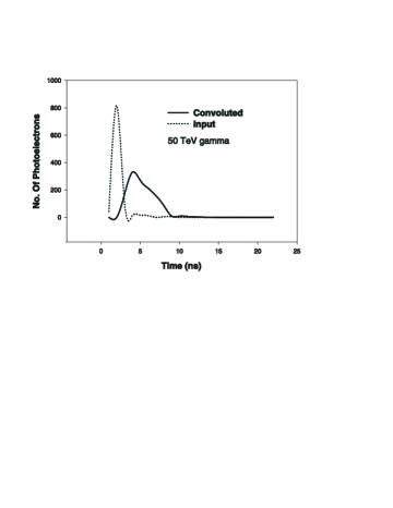
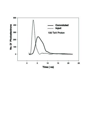
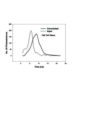
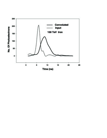
Figure 2: Pre-detector (input) and post-detector (convoluted) Cherenkov arrival time profiles for $\gamma$-ray, proton, neon and iron initiated showers.

It is important to study the shape of the Cherenkov photon arrival time distribution as represented by some pulse profile. So by fitting a suitable probability function, it is possible to parameterise the arrival time distribution. In most of the previous studies, generally, fittings have been done only at pre-detector state by using distributions like $\Gamma$-function and Lognormal functions. In the present study arrival-time distribution of the pe, obtained at the post-detector stage for each simulated event, has been fitted with exponentially modified Gaussian (emg) [22] and half-Gaussian modified Gaussian (gmg) [22] functions of the following forms, respectively: emg functions:

$$f(t)={\frac{ac\sqrt{2\pi}}{2d}}\exp[\frac{b-t}{d}+\frac{c^{2}}{2d^{2}}][\frac{d}{|d|}-{\rm erf}(z1)]$$ (9)

where

$$z1=\frac{b-t}{\sqrt{2}c}+\frac{c}{\sqrt{2}d}$$ (10)

gmg function :

$$f(t)={\frac{ac}{\sqrt{d^{2}+c^{2}}}}\exp[-\frac{1}{2}\frac{(t-b)^{2}}{d^{2}+c^{2}}][1+{\rm erf}(z)]$$ (11)

where

$$z=\frac{1}{2}\frac{\sqrt{2}d(t-b)}{c\sqrt{(d^{2}+c^{2})}}$$ (12)

The various properties of these two functions are Amplitude = $a$, Centre = $b$, area = $\sqrt{2\pi}ac$, FWHM = $2\sqrt{2ln2}c$, and time constant = $d$.
Both, emg and gmg functions have two small constraints, viz., c $>$ 0, and d $\neq$ 0. Rise time and base width ($t_{90}$ -$t_{10}$) which are obtained for each convoluted pulse profile has been determined.

Table 2: Average values of rise time and base width for gamma rays and hadrons in nanoseconds. The event distributions are shown in Fig. 3.

	gamma rays	protons	neon Nuclei	iron Nuclei
Rise Time	1.82	2.71	2.94	3.36
Base Width	7.29	8.50	9.37	10.06

While rise time as defined here is the time between 10$\%$ and 90$\%$ of the peak value, the base width is the time elapsed between 10$\%$ of peak value on both sides of the peak. We have used Table curve 2D (Jandel Scientific Software) [22] for fitting the above-referred two functions. Table 2 lists the mean values and the overall ranges of these

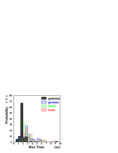
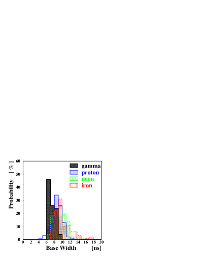
Figure 3: Rise time and base width parameters of Cherenkov arrival time pulse profiles (post-detector) for $\gamma$-ray, proton, neon and iron initiated showers.

parameters as derived for the simulated data. It is evident from both Figure 2 and Table 2 that $\gamma$-ray images have relatively smaller mean values, while iron nuclei have the largest values for these parameters, followed by neon nuclei and protons. Figure 3 depicts the distributions of rise time and base width for all species considered here.

8 U/V Spectral Ratio

Attention was first drawn by the Crimean Astrophysical Observatory group [23] towards the possible diagnostic role of the Ultraviolet (U; $\lambda\sim$ 250-310 nm) content of a Cherenkov event compared with the corresponding photon yield in the Visible (V; $\lambda\sim$ 310-500 nm) region – U/V spectral ratio – for differentiating between $\gamma$-rays and hadrons. The underlying rationale for this expectation is that, in case of $\gamma$-rays showers, the bulk of Cherenkov light is produced at relatively high altitudes ($\geq$ 8 km) by electron secondaries and the resulting light will be relatively deficient in the U-component because of rather strong atmospheric extinction effects for ultraviolet radiation coming from these altitudes. On the contrary, hadron showers are accompanied by relativistic muons which penetrate down to lower altitudes and generate relatively U-richer Cherenkov light closer to the observation plane. Different groups have expressed different and sometimes contradictory views about the efficacy of this parameter for event characterization purpose. The exact value for the U/V parameter for a given progenitor species is evidently a function of the

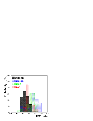
Figure 4: U/V ratio of $\gamma$-ray, proton, neon, and iron initiated showers at a typical distance of 195 m from the core.

actual detector configuration and spectral response as also the exact atmospheric conditions, apart from the effects of shower-to-shower fluctuations, etc. For practical reasons, the geometrical disposition of the U- and V- channel PMT and the detector size in the TACTIC instrument are not particularly favorable for measurements of the U/V parameters. Nevertheless, it is evident from Figure 4 that the expected distributions of this parameter for the TACTIC detector configuration are not completely overlapping and may as such help along with other parameters in separating $\gamma$-ray from hadrons.

9 ANN Studies

We have examined the implied classification potential of the above referred parameters more quantitatively by appealing to the pattern-recognition capabilities of an artificial neural network (ANN).
We have performed ANN studies by using the Jetnet 3.0 ANN package [24] with two Hillas parameters (W and D), two fractal dimensions ($D_{4}$, $D_{6}$), two wavelet moments ($\beta_{1}$, $\beta_{5}$), two time parameters (rise time, base width), and the U/V parameter as input observables. All the three hadron species have been taken together as a single cosmic-ray family. Thus the overall data-base used here consists of two types of events: 100 $\gamma$-rays and 300 hadrons, the latter consisting of proton, neon and iron nuclei taken in equal proportions. One half of the events have been used for training the ANN and the other half, for independently testing the trained net. For testing the stability of the net the training-testing procedures are repeated several times by varying the events belonging to the two samples. The output values demanded are 0.0 for $\gamma$-rays and 1.0 for hadrons. In all the ANN results discussed below, we have chosen

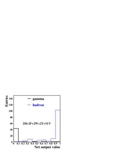
Figure 5: Event distribution of the neural net output of $\gamma$-rays and hadrons using all parameters corresponding to impact points of 195 m.

the net sigmoid function as $g(x)=1/(\exp{-2x}+1)$, with two hidden layers, one with 25 nodes and the other with 15 nodes. We have used the ANN in the back-propagation mode with a learning rate $\eta$=0.05 and the momentum parameter $\alpha$ = 0.5. For optimizing the cut value and checking the net quality there is a parameter called separability-index G [25], defined as
                  $G=\sqrt{\prod_{i=1}^{n}P_{i}}$
where n is the number of output classes (in our case, n=2) and $P_{i}$ denotes the probability of an event of class i to be classified in the right class. The maximum value of the G-index is 1.0 for an ideal segregation of the two classes. We calculate $G_{1}$ and $G_{2}$ which are the G-indices corresponding to the data of the training and testing samples, respectively.
For the examination of the separation quality of the net, we have trained the net with different parameters and their combinations of the mass sensitive observables (see Table 3). A multiparameter analysis method like neural net is able to find the best combination of different parameters. But if more parameters are used in the analysis the statistics of the Monte Carlo simulated events, necessary for training of the net, have to be increased in proportion (curse of dimensionality [26]). Hence the parameters with the least correlation have to be considered. The least correlated parameters from each set, i.e fractals, wavelets, Hillas-parameters etc., have been identified and results are given in Table  3. The similarity of the values of $G_{1}$ and $G_{2}$ indices indicates proper functioning of the net. The quality factor Q (ratio of $\gamma$-selection efficiency and the square root of the background selection efficiency) has been calculated for each case and corresponding values are given in the table which indicates that improved results are obtained for the case when imaging and non-imaging parameters are used together. The result of this last example is shown in Fig. 5. Similar ANN exercise has been repeated with all above mentioned parameters (except time due to non-availability of data) for data sets corresponding to core-distances of 245 m and 295 m. The results obtained are consistent with the corresponding results obtained at 195 m. From Table 3 it is clear that fractal parameters are better for $\gamma$/hadron separation than wavelet parameters for this small database. It is also evident that two time parameters (rise time and base width) show good segregation between $\gamma$-rays and hadrons and become more significant when combined with Hillas- , fractal- and wavelet parameters. On the other hand the U/V-ratio is a poor segregator but when used in combination with parameters of the other families it helps to improve the segregation quality. This behaviour is seen for all the three core distances.

Table 3: Details of the ANN studies. (–) means indeterminate values. The statistical uncertainties are in the order of $20\%$.

Set of parameters	Separability-index		Quality factor
	$G_{2}$	$G_{1}$	Q
2F	0.72	0.77	1.6
2W	0.66	0.66	–
2T	0.85	0.87	1.1
1UV	0.53	0.60	–
2H	0.65	0.70	–
2H+1UV	0.83	0.65	0.7
2H+2T	0.84	0.87	1.5
2H+2F	0.74	0.77	1.9
2H+2W	0.74	0.69	0.4
2H+2T+1UV	0.88	0.74	2.4
2H+2F+2T+2W	0.89	0.89	3.0
2H+2F+2T+2W+1UV	0.84	0.85	3.4

10 Discussion and Conclusions

The present exploratory study is remarkable for its deliberate choice of extremely small data-bases of $\gamma$-ray and hadron events and for seeking their efficient segregation through deployment of an unusually large number of parameters characterizing these events. An artificial neural network, having intrinsically superior and fault-tolerant cognitive capabilities and utilizing correlative features underlying these parameters for the net training and testing, is employed for achieving the desired classification. While as a sufficiently large data-base may help to properly train a neural net for $\gamma$-ray/hadron classification, based on only a limited number of event parameters, as demonstrated in the case of Hillas parameters by some previous authors, it is not expected to do so efficiently when the data-base size is restricted, as can happen in various practical situations. The latter view-point is clearly endorsed by the results presented in the first part of the previous section for various individual parameter families separately. The situation is found to improve favorably when several parameter families are used together and their underlying complementary properties exploited. The results presented here are remarkable in one respect, viz, $\gamma$-ray events are accepted at $>$ 90 $\%$ level, as compared to ($30-50\%$) $\gamma$-ray acceptance levels presently available through Hillas and supercuts image filter strategies. This significantly higher results of acceptance levels for $\gamma$-rays provided by the multiparameter approach, despite the extremely small data-base size, is of practical importance in ground-based $\gamma$-ray astronomy for the following two important reasons: The $\gamma$-ray source spectrum can be inferred with less ambiguity and/or lower-flux signals can be retrieved more efficiently. Another interesting observation made from the present study is that, since the ANN does not need large volumes of data ($\gamma$-rays or hadrons) for training when a sufficiently multi-dimensional parameter space is available, the necessary training can in principle, be imparted with actual (rather than simulated) $\gamma$-ray data, which any moderately sensitive experiment can record over a reasonable length of time from a known cosmic source, e.g., Crab Nebula, Mkn 501 or Mkn 421.
The following ’caveats’ need to be kept in mind in the context of the present exploratory work: Same primary energy (50 TeV for $\gamma$-rays and 100 TeV for the hadrons) has been considered. It would be in order to make a more realistic investigation involving ultra-high energy $\gamma$-rays and hadrons drawn from a typical spectrum and range of core distances going all the way to 500 m. Another related activity would be to seek the use of this enlarged parameter base for cosmic-ray mass composition studies as an extension of [5] and the present work and make it more definitive for handling real data going to be generated by the TACTIC array of Cherenkov telescopes. These studies are presently in progress and the results would be presented elsewhere.

References

- [1] T.C. Weekes et al., Astrophys. J. 342 (1989) 379
- [2] A.M. Hillas, Proc 19th ICRC (La Jolla) 3 (1985) 445
- [3] F.A. Aharonian et al., Astroparticle Physics 6 (1997) 369
- [4] D.J. Fegan, Proc. Int. Workshop ”Towards a Major Atmospheric Cherenkov Detector-I”, Paris (1992) p.3
- [5] A. Haungs et al., Astroparticle Physics 12 (1999) 145
- [6] B.M. Schäfer et al., Nucl. Instr. Meth. A 465 (2001) 394
- [7] C.L. Bhat et al., ”Towards a Major Atmospheric Cherenkov Detector-III”, Universal Academic Press 1994, ed. T.Kifune, p.207
- [8] J.N. Capdevielle et al., KfK-Report 4998, Kernforschungszentrum Karlsruhe (1990)
- [9] D. Heck et al., FZKA-Report 6019, Forschungszentrum Karlsruhe (1998)
- [10] C.L. Bhat et al., Nucl. Instr. Meth. A 340 (1994) 413
- [11] C.L. Bhat, Rapporteur Talk at the 25th ICRC (Durban), World Scientific 1997, eds. M.S. Potgieter, B.C. Raubenheimer, D.J. van der Walt, p.211
- [12] K. Werner, Phys. Rep. 232 (1993) 87
- [13] R.C. Rannot et al., Nucl. Phys. B (Proc. Suppl.) 52B (1997) 269
- [14] B.B. Mandelbrot, J. Fluid Mech. 62 (1974) 331
- [15] A. Aharony, Physica A 168 (1990) 479
- [16] A. Haungs et al., Nucl. Instr. Meth. A 372 (1996) 515
- [17] I. Daubechies, Commun. Pure Appl. Math. 41 (1988) 909
- [18] J.W. Kantelhardt, H.E. Roman, M. Greiner, Physica A 220 (1995) 219
- [19] M.D. Rodríguez-Frías, L. del Peral, J. Medina, Nucl. Instr. Meth. A 355 (1995) 632
- [20] O.T. Tumer et al., Nucl. Phys. B (Proc. Suppl) 14A (1990) 176
- [21] F.A. Aharonian et al., Astroparticle Physics 6 (1997) 343
- [22] Jandel Scientific software, Table Curve 2D, version 4 (1989), User’s Manual
- [23] A.A. Stepanian, V.P. Fomin, B.M. Vladimirsky, Izv. Krim. Ap. Obs. 66 (1983) 234
- [24] L. Lönnblad, C. Peterson, T. Rögnvaldsson, CERN Preprint, CERN-TH. 7135/94 (1994)
- [25] M. Roth, FZKA-Report 6262, Forschungszentrum Karlsruhe (1999)
- [26] C.M. Bishop, ”Neural Networks for Pattern Recognition”, Oxford University Press 1995