The morphological and dynamical evolution
of simulated galaxy clusters

We explore the morphological and dynamical evolution of galaxy clusters in simulations using scalar and vector-valued Minkowski valuations and the concept of fundamental plane relations. In this context, three questions are of fundamental interest: 1. How does the average cluster morphology depend on the cosmological background model? 2. Is it possible to discriminate between different cosmological models using cluster substructure in a statistically significant way? 3. How is the dynamical state of a cluster, especially its distance from a virial equilibrium, correlated to its visual substructure? To answer these questions, we quantify cluster substructure using a set of morphological order parameters constructed on the basis of the Minkowski valuations (MVs). The dynamical state of a cluster is described using global cluster parameters: in certain spaces of such parameters fundamental band-like structures are forming indicating the emergence of a virial equilibrium. We find that the average distances from these fundamental structures are correlated to the average amount of cluster substructure for our cluster samples during the time evolution. Furthermore, significant differences show up between the high- and the low-$\Omega_{\rm m}$ models. We pay special attention to the redshift evolution of morphological characteristics and find large differences between the cosmological models even for higher redshifts.

1 Introduction

Galaxy clusters may be thought to constitute a sort of pocket guide to our Universe: although they are small in comparison to cosmological scales, they contain important information about the Universe as a whole. One line of thought linking galaxy clusters and the background cosmology goes as follows: according to the hierarchical scenario, galaxy clusters were assembled through the merging of smaller objects, which collapsed first. Richstone et al. (1992) suggested that the cluster dynamical state is related to its age, which in turn depends on average on the present value of the cosmological density parameter $\Omega_{{\rm m}}$. If, finally, the cluster dynamical state is mirrored by its substructure, one can establish a link between cluster morphology and the background cosmology (“cosmology-morphology connection for galaxy clusters”, Evrard et al. 1993). Therefore, the cluster substructure may be a powerful tool to study the background cosmology. Summarising the results of the theoretical analyses (see also Bartelmann et al. 1993), one can state that in low-$\Omega_{{\rm m}}$ cosmologies the clusters should on average show a smaller amount of substructure than in high-$\Omega_{{\rm m}}$ models. Since this argument oversimplifies the complex dynamical situation in galaxy clusters, it has to be complemented using simulations, see e.g. (Evrard et al. 1993). Note, that we need a thorough definition and description of cluster substructure for this argument.
In this context, it is still a difficult task to describe both the inner cluster state and the cluster morphology quantitatively in a reliable way. – In this paper, therefore, we use new tools to quantify cluster substructure as well as the intrinsic cluster state. We analyse cluster simulations with these tools and characterise the substructure of different cluster components, its relation to inner cluster properties and the differences between cosmological background models as traced by the averaged cluster substructure. In particular, we test the theoretical assumptions behind the “cosmology-morphology connection”.
So far, various methods have been used to quantify the amount of substructure in galaxy clusters. In the optical band several techniques (Dressler & Shectman 1988; West & Bothun 1990; Bird 1994) use the galaxy positions and velocities. Other methods are based on the hierarchical clustering paradigm (Serna & Gerbal 1996; Gurzadyan & Mazure 1998), wavelet analysis (Girardi, M., Escalera, E., Fadda, D., et al. 1997), or moments of the X-ray photon distribution (Dutta 1995).
X-ray images of galaxy clusters were also used to study substructure; contrary to optical clusters, they are scarcely contaminated by fore- and background effects. Mohr et al. (1995) applied statistics based on the axial ratio and the centroid shift of isophotes  (Mohr et al. 1993) to a sample of Einstein IPC cluster images. Buote & Tsai (1995) introduced the power ratio method, a technique based on the multipole expansion of the two-dimensional potential generating the observed surface X-ray brightness, see also Buote & Tsai (1996); Buote & Xu (1997); Tsai & Buote (1996); Valdarnini et al. (1999). Kolokotronis et al. (2001) studied the correlation between substructures observed both in the optical and X-ray bands.
Cosmological N-body simulations have been used to test the dependence of cluster substructure on different cosmological models (Evrard et al. 1993; Mohr et al. 1995; Jing et al. 1995; Thomas, P. A., Colberg, J. M., Couchman, H. M. P., et al. 1998; West et al. 1988). Crone et al. (1996) applied different substructure statistics to galaxy clusters obtained in different cosmological models from numerical simulations. They conclude that the “centre-of-mass shift” is a better indicator to distinguish between different models than, e.g., the Dressler Shectman statistics (Dressler & Shectman 1988), which does not provide significant results (Knebe & Müller 2000). Pinkney et al. (1996) tested several descriptors using N-body simulations and recommended a battery of morphology parameters to balance the disadvantages of different methods.
So far, however, a unifying framework for the morphological description of galaxy clusters is missing. Several aspects of cluster substructure have to be distinguished in order to provide an exhaustive characterisation. Also the connection to a possible cluster equilibrium has not yet been scrutinised.
In this paper we apply Minkowski valuations (MVs) (Mecke et al. 1994; Beisbart et al. 2001a, b) to cluster substructure and use fundamental structures to quantify the dynamical state of galaxy clusters. The Minkowski framework provides mathematically solid and unifying morphometric concepts, which can be applied to cluster data without any statistical presumptions. These measures distinguish effectively between different aspects of substructure and discriminate between different cosmological background models. Our interest is both methodological and physical: on the one hand, we are looking for an appropriate method to quantify cluster substructure; on the other hand, we ask physical questions like: how are the Dark Matter (DM) and the gas distribution related to each other?
For our investigation, we employ combined N-body/hydrodynamic simulations. This simulation technique is particularly suitable for our purposes, since it traces both the dark matter and the gas component of a cluster. We construct relatively large data bases of cluster images from the simulations which can be compared to real cluster images.
The plan of the paper is as follows: after an explanation of the simulations and cosmological models in Sect. 2, we give an introduction into Minkowski valuations in Sect. 3. We employ these tools in Sect. 4 in order to compare the clusters within the different simulations. An analysis of fundamental plane relations is presented in Sect. 5. We draw our conclusions in Sect. 6.

2 The cosmological models and the simulations

In order to investigate cluster substructure in different cosmological models, a data base of galaxy clusters was generated on the base of TREESPH simulations. Three background cosmologies were chosen differing both in terms of the values of the cosmological parameters and the power spectra. We restricted ourselves to CDM models; the simulations are described in more detail in Valdarnini et al. (1999), where also a morphological analysis was done using the power ratios (PRs, see Buote & Tsai 1995). We extend this work in several directions, e.g. by probing the morphological evolution and by connecting cluster substructure and inner dynamical cluster state.
Since observations indicate that the curvature parameter $\Omega_{\rm K}$ vanishes (see for instance de Bernardis, P., Ade, P. A. R., Bock, J. J., et al. 2000) we considered three spatially flat cosmological models, namely two high-$\Omega_{\rm m}$ models (a standard Cold Dark Matter model – CDM – and a model where the Dark Matter consists of a mixture of massive neutrinos and Cold Dark Matter – CHDM) and one low-$\Omega_{\rm m}$ model (a model with a non-vanishing cosmological constant – $\Lambda$CDM). For the Hubble parameter we chose $h=0.5$ for the CDM and the CHDM model, and $h=0.7$ for the $\Lambda$CDM model; here, as usual, the Hubble constant is written in the form $H_{\rm 0}=100\,h\,{\rm\mbox{km}\,\mbox{s}}^{-1}\,{\rm\mbox{Mpc}}^{-1}$.
With respect to the power spectra comprising the influence of the initial matter composition on structure formation we adopted a primeval spectral index of $n=1$ and selected a baryon density parameter of $\Omega_{\rm b}h^{2}=0.015$. In the CHDM  model we had one massive neutrino with mass $m_{\nu}=4.65\,$eV, yielding a HDM density parameter $\Omega_{\rm h}=0.2$. In the $\Lambda$CDM  model the vacuum contribution to the energy density was $\Omega_{\Lambda}=0.7$ in accordance with recent observations of Supernovae (Perlmutter, S., Aldering, G., Goldhaber, G., et al. 1999). Therefore, the density parameter of matter $\Omega_{{\rm m}}$ was $1$ for CDM and CHDM, and $0.3$ for $\Lambda$CDM. Since we are dealing with galaxy clusters and need a fair number of them, all models were normalised in order to match the present-day cluster abundance $n_{\rm c}(M>M_{\rm c})=4\cdot 10^{-6}h^{3}$ for $M_{\rm c}=4.2h^{-1}10^{14}M_{\odot}$ (Eke et al. 1996; Girardi, M., Escalera, E., Fadda, D., et al. 1997). Using these normalisations only the $\Lambda$CDM model is consistent with the measured COBE quadrupole moment at the $1\sigma$ level. In order to reduce the influence of cosmic variance the same random numbers were used to set the initial conditions for all cosmological models. Therefore we roughly look at the same clusters in all cosmologies.
The cluster simulation technique consisted of two steps: first for each model a large collisionless N-body simulation was performed using a P³M code in a box of length $L=200\,a\,h^{-1}{\rm\mbox{Mpc}}$, where $a$ is the cosmological scale factor being one at present day. We considered $N_{\rm p}=10^{6}$ particles for the CDM and CHDM  models, each, while $N_{\rm p}=84^{3}$ particles were chosen for the $\Lambda$CDM model, the only low-density cosmology investigated here; thus the mass of one simulation particle is approximately equal in all cosmological models. The simulations were run starting from an initial redshift $z_{\rm in}$, depending on the model (for more details see Valdarnini et al. 1999), down to $z=0$. At the final redshift we identified galaxy clusters using a friend-of-friend algorithm in order to detect overdensities in excess of $\simeq 200\,\Omega_{{\rm m}}^{-0.6}$. For our further analyses, we took into account only the $40$ most massive clusters.
As a second step we applied a multi-mass technique (Katz & White 1993; Navarro et al. 1995): for each cluster we carried out a hydrodynamic TREESPH simulation in a smaller box starting from $z_{\rm in}$. For this we identified all cluster particles within $r_{\rm 200}$ (where the cluster density is about $200\,\Omega_{{\rm m}}^{-0.6}$ times the background density) at $z=0$. These particles were backtracked to $z_{\rm in}$ in the original cosmological simulation box. For each cluster a cube enclosing all of these particles was constructed; its size $L_{\rm c}$ was ranging from $15$ to $25h^{-1}{\rm\mbox{Mpc}}$. A higher-resolution lattice of $N_{\rm L}=22^{3}$ grid points then was set into these cubes. Different lattices were used for the different mass components; to avoid singularities these lattices were shifted with respect to each other by ${1/2}$ of the grid constant along each spatial direction. For the CHDM  simulations the hot particles bear a small initial peculiar velocity following a Fermi-Dirac distribution with Fermi velocity $v_{\rm 0}=5(1+z_{\rm in})(10{\rm eV}/m_{\nu})$ km s^-1. For the gas particles we started with an initial temperature $T_{\rm i}=10^{4}{\rm K}$. The TREESPH simulation was then run using all particles which lie inside a sphere of radius $L_{\rm c}$ around the centres of the cubes.
The gravitational softening parameters $\varepsilon$ were the same for all clusters within each simulation and cosmological model. For the gas particles they were chosen to be $\varepsilon_{\rm gas}=80,\,100\,,60\,\leavevmode\nobreak\ {\rm\mbox{kpc}}$ for the CDM, the CHDM , and most of the $\Lambda$CDM  clusters, respectively. However, for the five most massive $\Lambda$CDM  clusters $\varepsilon_{\rm gas}$ was set to 80   kpc. As softening parameters for the Dark Matter particles we took $\varepsilon_{\rm d}=200,231,125$ kpc for the CDM, CHDM, and $\Lambda$CDM  model, respectively. For the simulation particles we applied the scaling $\varepsilon_{\rm i}\propto m_{\rm i}^{1/3}$. Note, that the softening lengths were fixed within proper physical space; however, the redshift $z_{in}$ is chosen in such a way, that the mean particle separation is always smaller than the softening length. The spatial resolution of the simulations can be estimated by the ratio $\varepsilon_{\rm gas}/r_{\rm 200}$, which never exceeds a value of about $0.04$.
The numerical integrations were performed with a tolerance parameter $\theta=0.7$ and using a leap-frog scheme for the time integration; the minimum time step allowed was $3\times 10^{6}$ years for the gas particles and $6\times 10^{6}$ years for the DM part. Viscosity was treated as in Hernquist & Katz (1989) with $\alpha=1$ and $\beta=2$. The effects of heating and cooling were not considered in the simulations. Tests assessing the quality of the simulations are described in Valdarnini et al. (1999). We saved numerical outputs at different redshifts, such that the cluster morphological evolutions could be investigated within the different models.
Using the simulations we generated cluster images which mimic observations in a realistic manner as follows: the gas density was estimated on a cubic grid with a grid constant of $0.03\leavevmode\nobreak\ h^{-1}{\rm\mbox{Mpc}}$ for each model. We took the square of this density at each grid point and calculated the approximate integral of $\rho^{2}$ along the line of sight orthogonal to a random plane (it is the same random plane for all clusters, simulations, and redshifts), with $101\times 101$ pixels. We considered the cluster as approximately isothermal, such that the X-ray emissivity is just proportional to this integral (see, e.g., Tsai & Buote 1996).
We applied the same method also to the DM particles; evidently, this does not lead to a physically observable quantity. However, in this way we get the emissivity we

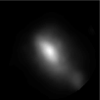
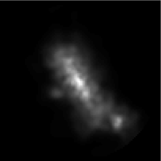
Figure 1: Two of the simulated cluster images to be analysed. They show the X-ray image of one cluster in the $\Lambda$CDM model at redshift zero (left panel) and the corresponding pseudo-DM-image, where the gas density has been replaced by the DM-density (right panel). Both images are sampled within a circle of radius $1.5h^{-1}{\rm\mbox{Mpc}}$ around the peak of the gas/DM-surface brightness, respectively. See the main text for a further description of the image construction.

would obtain if the gas distribution would trace the DM (a constant ratio between gas and DM distribution drops out in our analysis). We show both an X-ray and a DM-image in Fig. 1. The images are analysed using the Minkowski valuations, which are described in the next section.

3 Minkowski valuations

The Minkowski valuations (MVs) provide an elegant and in a certain sense unique description of spatial data. They were introduced into cosmology by Mecke et al. (1994) and have been applied to answer a number of questions regarding the morphology of the large-scale structure, see, e.g. Kerscher, M., Schmalzing, J., Retzlaff, J., et al. (1997); Kerscher et al. (1998); Schmalzing & Gorski (1998); Sahni et al. (1998); Schmalzing, J., Buchert, T., Melott, A. L., et al. (1999); Kerscher, M., Mecke, K. Schmalzing, J., et al. (2001). So far, they were employed mainly in situations where perturbations of a homogeneous background were to be expected and the amount of clustering had to be quantified. For galaxy clusters, however, the situation is different. Galaxy clusters are intrinsically inhomogeneous systems, thus the main issue is how far their structure is away from a symmetric and substructure-poor state which does not show the influence of recent mergers.
For this reason, additionally to the scalar Minkowski functionals, we use vector-valued Minkowski valuations (also known as “Quermaß vectors”), which feature directional information. In this section we give a short overview of both the scalar and the vector-valued MVs.
For a general approach, let us consider patterns $P,Q,...$, i.e. compact sets within Euclidean space. A morphometric (geometrical and topological) description of such spatial patterns is adequate, if it obeys a number of covariance properties specifying how the descriptors change if the pattern is transformed. The Minkowski valuations are defined by three types of covariances.

1. The first class of covariance refers to motions in space: a morphological descriptor should behave in a well-defined way, if the pattern is moved around in space. The scalar Minkowski functionals are motion-invariant, whereas the vector-valued MVs transform like vectors (motion equivariance).

2. Secondly, the descriptors should obey a simple rule specifying how they sum up for combined patterns whose set union is constructed. Both classes of Minkowski valuations $V$ obey the additivity:

   $$V(P\cup Q)=V(P)+V(Q)-V(P\cap Q)\;\;\;.$$ (1)

3. Moreover, continuity states that a descriptor should change continuously if the pattern is distorted slightly.

These simple properties already define the MVs, since – at least on the convex ring the Theorem of Hadwiger (Hadwiger 1957; Hadwiger & Schneider 1971) guarantees that in $d$ dimensions, only $(d+1)$ of such measures – either scalar- or vector-valued ones – are linearly independent.
Because of the structure of our cluster data, we concentrate on the case of $d=2$. Here, the Minkowski functionals have intuitive meanings: $V_{0}$ is the surface content of the pattern, $V_{1}$ its length of circumference, and $V_{2}$ its Euler characteristic $\chi$, which counts the components of the cluster and subtracts the number of holes. Note, that all of these functionals can be expressed as an integral: $V_{0}$ obviously is the two-dimensional volume integral of the pattern, $V_{1}$ is its (one-dimensional) surface integral, and $V_{2}$ weights each surface element ${\rm d}S$ with the local curvature $\kappa$. This integral representation is also valid for the vector-valued Minkowski valuations; in this case, additionally, the integrals are weighted with the position vector; therefore, the Quermaß vectors are spatial moments of the scalar Minkowski functionals. Summarising we consider the following measures:

$$V_{0} =\int_{P}{\rm d}V\;\;\;,\quad \@vec{V}_{0} =\int_{P}{\rm d}V\@vec{x}\;\;\;,$$ (2)

$$V_{1} =\int_{\partial P}{\rm d}S\;\;\;,\quad \@vec{V}_{1} =\int_{\partial P}{\rm d}S\@vec{x}\;\;\;,$$

$$V_{2} =\int_{\partial P}{\rm d}S\kappa\;\;\;,\quad \@vec{V}_{2} =\int_{\partial P}{\rm d}S\kappa\@vec{x}\;\;\;,$$

where $\kappa$ refers to the local curvature. – It is convenient to divide the vectors by the corresponding scalars to arrive at the (curvature) centroids:

$$\@vec{p}_{i}\equiv\frac{\@vec{V}_{i}}{V_{i}}\;\;\;.$$ (3)

The centroids localise individual morphological features. In particular, they coincide with the symmetry centre for spherically symmetric patterns. On the other hand, centroids constituting a finite triangle indicate the presence of asymmetry.
Note, that the MVs obey covariance properties with respect to a scaling of the pattern $P$, too: If we scale the pattern by $\alpha>0$ to get $\alpha P=\{\alpha\@vec{x}|\@vec{x}\in P\}$, the scalar Minkowski functionals transform like $V_{i}(\alpha P)=\alpha^{d-i}V_{i}(P)$; the vectors transform like $\@vec{V}_{i}(\alpha P)=\alpha^{d-i+1}\@vec{V}_{i}(P)$. This is important since we sometimes have to compare data of different size.
Obviously, cluster images are not patterns in the above sense, but rather consist of galaxy positions or pixelised maps reflecting the surface brightness within a certain energy band. Thus, we have to construct patterns from the cluster data. Here we use the excursion set approach where we smooth the original data using a Gaussian kernel in order to construct a realization of a field $u(\@vec{x})$. The excursion sets

$$M_{w}=\{\@vec{x}|u(\@vec{x})>w\}\;\;\;.$$ (4)

are analysed with the aid of the Minkowski valuations. Varying the density threshold $w$ allows us to probe different regions of the cluster. The smoothing both reduces possible noise and picks out a scale of interest or resolution beneath which substructure is no longer resolved.
The MVs, represented as functions of the density threshold, contain very detailed information. In this paper, however, we want to compare cluster images drawn from a larger base of simulated galaxy clusters. We are therefore interested in the average morphological cluster evolution in different cosmologies. In order to condense the detailed information present in the MVs, we construct robust structure functions which allow us to compare clusters of different size statistically.
This can be done by integrating over the density thresholds and weighting with functions of the Minkowski valuations. We define an average over different density thresholds via

$$\left\langle f\right\rangle_{\rm u}\equiv\frac{1}{u_{\rm max}-u_{\rm min}}\int_{u_{\rm min}}^{u_{\rm max}}{\rm d}uf\;\;\;.$$ (5)

Here, we consider three classes of robust structure functions, which feature different aspects of the substructure and span a morphological phase space. We distinguish the following three classes of substructure, which are quantified using one or more structure functions:

1. the clumpiness $C\equiv\sqrt{\left\langle(\chi-1)^{2}\right\rangle_{\rm u}}$ is a measure of the number of subsystems in a cluster;

2. the shape and asymmetry parameters ($A_{0}\equiv\left\langle{\rm Area}(\triangle(\@vec{p}_{j}))\right\rangle_{\rm u}$, $A_{1}=\left\langle{\rm perimeter}(\triangle(\@vec{p}_{j}))\right\rangle_{\rm u}$) refer to the degree of asymmetry and the global shape of the cluster (“is the cluster spherical or elongated?”); here we use the fact that curvature centroids which do not coincide within one point indicate the presence of asymmetry. In particular, the size of the triangle $\triangle(\@vec{p}_{j})$ which connects the curvature centroids (measured by its area and perimeter) serves as a measure of the asymmetry present within the cluster.

3. the shift parameters $S_{i=0,1,2}\equiv\sqrt{\left\langle|\@vec{p}_{i}-\left\langle\@vec{p}_{i}\right\rangle_{\rm u}|^{2}\right\rangle_{\rm u}}$ account for the variation or shift of morphological properties in a quantitative way by considering different density thresholds (these parameters are generalisations of the frequently used centre-of-mass shift and centroid variation, see Crone et al. (1996); Mohr et al. (1993, 1995)).

An effective method to calculate Minkowski valuations from pixelised maps can be developed in analogy to Schmalzing & Buchert (1997) and is given in  Beisbart, C., et al. (2001).

4 Cluster substructure and the background cosmology

To start our analysis of the simulated clusters, we probe the connection between the background cosmology and the cluster morphology. Since in this case not so much the substructure of individual clusters rather than the mean morphology is of interest, we define cluster samples consisting of all clusters at one redshift within one model (unless otherwise stated we analyse one random projection per cluster). In order to trace the mean substructure evolution, we average the structure functions over all clusters within one sample.
What is the amount of cluster substructure, and how does it evolve within the three cosmological models? – The simulated clusters are “observed” within a quadratic window of $3h^{-1}{\rm\mbox{Mpc}}$ width centred at the peak position of the surface brightness. The data are smoothed using a Gaussian kernel with different smoothing lengths in order to reduce the sensitivity to noise and to probe different scales of the substructure. We concentrate on intermediate values of the smoothing scale $\lambda$ ($\lambda\sim 0.05-0.15h^{-1}{\rm\mbox{Mpc}}$, Cen (1997) employs values of the same order of magnitude). To define the cluster on the image, we draw circles around the peak with radii $r_{\rm w}=0.8,1.0,1.2,1.4h^{-1}{\rm\mbox{Mpc}}$ (this definition is in the spirit of Abell’s cluster identification in the optical, see Abell 1958, we call this circle the cluster window) and neglect the rest. The integration limit $u_{\rm min}$ in Eq. (5) is chosen to be twelve times the background which is determined from the rest of the image similarly as in Böhringer, H., Voges, W., Huchra, J., et al. (2000), $u_{\rm max}$ in Eq. (5) is the maximum cluster surface brightness.
In Fig. 2 we show results for the X-ray cluster

Figure 2: The averaged morphological evolution of the galaxy clusters in our three cosmological models. The ensemble-averaged structure functions clumpiness, shape and asymmetry, and shift of morphological properties were determined from the X-ray luminosity for a smoothing length of $\lambda=0.05h^{-1}{\rm\mbox{Mpc}}$ and are shown vs. redshift (first row). CDM: solid line; CHDM: short dashed line; $\Lambda$CDM: long dashed line.  We consider a spherical window with radius $r_{\rm w}=1.4h^{-1}{\rm\mbox{Mpc}}$; C is dimensionless; A₁ and S₁ are given in units of $(h^{-1}{\rm\mbox{Mpc}})^{2}$ and $h^{-1}{\rm\mbox{Mpc}}$, respectively. In the second row we show the A${}_{1}^{\prime}$ and S${}_{1}^{\prime}$, where A₁ and S₁ were scaled to cluster size (an estimate of the half light radius) in order to get dimensionless parameters.

morphology within the three models having applied a smoothing length of $0.05\leavevmode\nobreak\ h^{-1}{\rm\mbox{Mpc}}$. A couple of things are obvious at first glance: there is a significant difference between the high-$\Omega_{\rm m}$ models (CDM and CHDM) and the low-$\Omega_{\rm m}$ model ($\Lambda$CDM). These differences are visible in most of the structure functions and are in accordance with the theoretical expectations: the low-$\Omega_{\rm m}$ model shows by far less substructure than the other two models – at least for most redshifts investigated here. The CDM and CHDM models, however, do not seem to be distinguished well. Therefore, the morphology-cosmology connection is mainly sensitive to the values of the cosmological parameters, but performs poorly in discriminating between different power spectra. The clumpiness is particularly sensitive. – Regarding the redshift evolution, a clear trend is visible towards more relaxed and substructure-poor clusters. In particular, there are also large morphological differences between the models at higher redshifts. Morphological evolution of galaxy clusters may therefore serve as a more sensitive test than the present-day cluster morphology. Note, that the averaged morphology evolution still looks relatively spiky. The reason is that for individual clusters the evolution of the structure functions proceeds in a discontinuous manner, when subclumps enter the cluster window. Therefore, one has to average over several clusters in order to get a typical morphological cluster evolution.
The structure functions A_i and S_i have a dimension and therefore quantify the absolute amount of substructure. To investigate the substructure relative to cluster size, we normalise A₁ and S₁ to the individual cluster size estimated via the two-dimensional half-light radius around the peak of the X-ray surface brightness. As visible from the bottom row of Fig. 2, the qualitative evolution and the differences between the models are similar as before.

Figure 3: The morphological evolution of the DM within the clusters. The ensemble-averaged structure functions clumpiness, shape and asymmetry, and shift of morphological properties for a smoothing length of $0.05h^{-1}{\rm\mbox{Mpc}}$ are shown vs. redshift. CDM: solid line; CHDM: short dashed line; $\Lambda$CDM: long dashed line.  Contrary to Fig. 2, here we probe the DM. We consider a spherical window of radius $r_{\rm w}=1.4h^{-1}{\rm\mbox{Mpc}}$; for the units see the caption of Fig. 2. This time, we also show the one-sigma fluctuations around the average structure functions for the $\Lambda$CDM model. Note, that large fluctuations are to be expected on physical grounds because of the wide range of clusters investigated, having different formation times and environments. We conclude that one has to consider the whole morphology distribution within the samples in order to get significant claims regarding the background cosmology (see below).

So far we concentrated on the morphological evolution as traced by the X-ray luminosity and thus the X-ray gas. But is also the DM morphology different for the cosmological models? The results in Fig. 3 show the mean substructure evolution for galaxy clusters ($\lambda=0.05h^{-1}{\rm\mbox{Mpc}}$) and indicate that the DM morphology in clusters is even more sensitive to the cosmological background than the gas.
In order to strengthen our claims and to compare the performance of the gas- and the DM-morphology in a systematic way, we take into account the whole distribution of the structure functions for our cluster samples. The Kolmogorov-Smirnow test is a suitable tool to answer the question whether two data samples are likely to be drawn from the same distribution. It measures the distance between two cumulative distributions $D_{1}(X)=p(x<X)$ and $D_{2}$ (estimated from the empirical data) via

$$d_{\rm KS}=\underset{x\in{\mathbb{R}}}{{\rm max}}\{|D_{1}(x)-D_{2}(x)|\}\;\;\;.$$ (6)

For any value of $d_{\rm KS}$ one can estimate the probability $p_{\rm KS}$ that the same random process generates two samples being “farther away” from each other than $d_{\rm KS}$. If $d_{\rm KS}$ is large and, accordingly, $p_{\rm KS}$ is small, the distributions under investigation are likely to stem from two different ensembles.

Table 1: The discriminative power of the structure functions regarding the cosmological background models. The X-ray morphology is considered for a smoothing length of $\lambda=0.05h^{-1}{\rm\mbox{Mpc}}$ and at redshift zero. For each pair of background models, we calculate the Kolmogorov-Smirnow distance $d_{\rm KS}$ between the distributions of the structure functions as well as the probability of the nullhypothesis. As one can see, the gas substructure clearly discriminates between the high- and the low-$\Omega_{\rm m}$ models.

Gas, $r_{\rm w}=1.40h^{-1}{\rm\mbox{Mpc}},\,z=0,\,\lambda=0.05h^{-1}{\rm\mbox{Mpc}}$
	CDM – $\Lambda$CDM		CHDM – $\Lambda$CDM		CDM – CHDM
	$d_{\rm KS}$	$p_{\rm KS}$	$d_{\rm KS}$	$p_{\rm KS}$	$d_{\rm KS}$	$p_{\rm KS}$
C	0.29	7.7 %	0.31	4.5 %	0.17	57.7 %
A1	0.35	1.6 %	0.40	0.4 %	0.12	91.4 %
S1	0.36	1.2 %	0.38	0.7 %	0.15	71.8 %

Table 1 presents results of a KS test for redshift $z=0$ and a smoothing length of $\lambda=0.05h^{-1}{\rm\mbox{Mpc}}$. The small values of $p_{\rm KS}$ show that the distinction of the cosmological models by means of the structure functions is effective regarding the values of the cosmological parameters. A systematic imprint of the power spectrum on cluster morphology, however, does not seem to be noticeable. The DM is even better than the gas in discriminating between the background cosmologies. For instance, in comparing the CDM and the $\Lambda$CDM model, the probability of the null hypothesis is smaller than $10^{-5}$ using the clumpiness ($\lambda=0.1h^{-1}{\rm\mbox{Mpc}}$).
So far, we investigated only one smoothing scale and one size of the cluster window; but one may ask which cluster regions are most interesting for a distinction between cosmological models and which smoothing lengths are optimal for our purposes. In order to answer these questions, we first focus on the gas and estimate our structure functions for all cluster samples at redshift $z=0$ for a number of smoothing lengths and scales of the cluster window. For each window and smoothing scale we calculate the KS-distances between our three models. The results show that for the clumpiness small smoothing lengths $\lambda$ are more favourable than larger ones. For lower resolutions, therefore, the subclumps are smeared out, and the clumpiness is dominated by random fluctuations.
On the other hand, the discriminative power of the clumpiness is enhanced for larger scales of the window. The reason is that subclumps which have not yet merged with the main cluster component are to be found at the outer cluster parts. The other structure functions mostly depend only relatively weakly on the window scale. We conclude that the outer cluster regions, which probably have not yet been virialised, are of more interest for the cosmologist. Moreover, the values of the structure functions rise for larger windows. This confirms results by Valdarnini et al. (1999), who found a similar behaviour (see, e.g., their Table 5). For the DM morphology one obtains comparable results.

5 Fundamental plane relations

Using cluster simulations one can test the basic assumption behind the morphology-cosmology connection presuming that the morphology of a cluster mirrors its inner dynamical state reliably. In this section we try to bring together morphology and inner state of our galaxy clusters. Mostly, we focus on the $\Lambda$CDM model as the nowadays favoured one.
Observationally there is evidence that clusters of galaxies undergo a dynamical evolution leading to a sort of equilibrium. This equilibrium seems to be manifest in fundamental plane relations holding within three-dimensional spaces of global cluster parameters where clusters tend to populate a plane. Since the cluster parameters are logarithms of observable quantities, the fundamental plane (FP) corresponds to a power law constraint among the real cluster parameters. Usually fundamental plane relations are explained in terms of the virial theorem of (Chandrasekhar & Lee 1968), which, however, is strictly valid only for isolated systems (for a discussion see Fritsch & Buchert 1999).
There are several interesting spaces of global cluster parameters, depending on whether optical or X-ray data are available. Usually, the scale of the cluster, an estimate of its mass and a quantity related to its kinetic energy like the velocity dispersion of the galaxies or the temperature of the X-ray emitting gas are considered, see, e.g., Schaeffer et al. (1993); Adami et al. (1998) for optical fundamental planes and Annis (1994); Fritsch & Buchert (1999); Fujita & Takahara (1999) for X-ray clusters. In each case, indirectly, the potential and the kinetic energy are referred to.
Fritsch & Buchert (1999) showed that the substructure of a cluster is correlated to its distance from the fundamental plane using the COSMOS/APM and the ROSAT data. In the spirit of their work, we try to establish a similar connection for simulated X-ray clusters.

5.1 Fundamental plane relations for the simulated clusters

Table 2: Summary of the cluster parameter spaces investigated: the $i$th parameter space is spanned by the parameters $P_{i}^{j=0,1,2}$ for $i=1,..,3$.

Par. Space $i$	Parameters $P_{i}^{j}$
No.	$j=0$	$j=1$	$j=2$
$i=1$	$\log\left(M_{200}/(10^{15}h^{-1}M_{\sun})\right)$	$\log\left(r_{\rm h}/(100h^{-1}{\rm\mbox{kpc}})\right)$	$\log\left(T/(10^{7}{\rm\mbox{K}})\right)$
$i=2$	$\log\left(M_{200}/(10^{15}h^{-1}M_{\sun})\right)$	$\log\left(r_{\rm h}/(100h^{-1}{\rm\mbox{kpc}})\right)$	$\log\left(L_{\rm X}/(10^{43}{\rm ergs}^{-1}h^{-2})\right)$
$i=3$	$\log\left(M_{200}/(10^{15}h^{-1}M_{\sun})\right)$	$\log\left(r_{\rm h}/(100h^{-1}{\rm\mbox{kpc}})\right)$	$\log\left(\sigma_{\rm v}/(10^{2}{\rm\mbox{km}\;s}^{-1})\right)$

Using our simulated clusters, we test three possible parameter spaces spanned by: 1. the mass, the half-light-radius, and the emission-weighted X-ray temperature; 2. the mass, the half-mass-radius, and the X-ray luminosity; 3. the mass, the half-mass-radius, and the velocity dispersion. In all of those global parameter spaces, one can observe a band-like fundamental structure. This thin band may be fitted either by a plane or a line. In Table 2 the global cluster parameters are summarised using a compact notation which we will use from now on.
The parameters defining the different cluster parameter spaces are estimated from the simulations as follows: the cluster mass is quantified via $M_{200}$ contained within an overdensity $\delta_{\rm c}$ times the critical density $\rho_{\rm c}$ : $M_{200}=\frac{4\pi}{3}\delta_{\rm c}\rho_{\rm c}r_{200}^{3}$, where $\delta_{\rm c}\simeq 178\cdot\Omega_{{\rm m}}^{-0.45}$ in a flat cosmology (Coles & Lucchin 1994) and where $r_{200}$ is the size of this overdensity. $r_{200}$ as well as $r_{\rm h}$ are determined from the three-dimensional mass distribution around the density maximum, $r_{\rm h}$ is the half-mass radius. $T_{\rm em}$ denotes the emission-weighted temperature of the gas, calculated from the gas thermal energy assuming an ideal gas. The bolometric X-ray luminosity is defined as $L_{\rm X}=\int{\rm d}V(\frac{\rho_{\rm gas}}{\mu m_{\rm p}})^{2}\Lambda_{\rm c}$, where $\rho_{\rm gas}$ is the gas density, $\mu=0.6$ the mean molecular weight, $m_{\rm P}$ the proton mass, and $\Lambda_{\rm c}$ the cooling function. In order to perform the volume integration, the standard SPH estimator has been applied (Navarro et al. 1995), the summation includes all particles within the virial radius $r_{200}$. The velocity dispersion is estimated from all types of simulation particles.
Before investigating the relationships between these parameters, we ask whether the distributions of these parameters are consistent with each other for the different cosmological models (in the sense of the KS test). We find consistency apart from the luminosity (which is higher on average for the $\Lambda$CDM model) and the half-light radius (clusters seem to be more compact within the CHDM model).
We fit a plane and a line to each cluster sample separately (one sample means one cosmological model at one redshift) using an orthogonal distance regression, see Boggs et al. (1987, 1989); this technique treats all variables the same way, i.e. no parameter is a priori thought of as dependent on the others. The planes are parametrised by

$$i{\rm th\;plane} i$$ (FP )

$$P_{i}^{0}+\beta_{i}^{1}P_{i}^{1}+\beta^{2}_{i}P_{i}^{2}=\beta^{3}_{i}\;\;\;,$$

the lines are defined via:

$$i{\rm th\;line} i$$ (FL )

$$\begin{split}P_{i}^{1}&=\gamma_{i}^{1}P_{i}^{0}+\gamma_{i}^{3}\\ P_{i}^{2}&=\gamma_{i}^{2}P_{i}^{0}+\gamma_{i}^{4}\;\;\;.\end{split}$$

We call the best-fitting planes and lines fundamental planes/fundamental lines, respectively.
We show one of the fundamental structures in Fig. 4 at redshift $z=0$ for the $\Lambda$CDM model. To get a clearer representation, we fit a second plane to our data under the constraint, that it be orthogonal to the fundamental plane, as Fujita & Takahara (1999) did. A second constraint equation among the cluster parameters should force the clusters to lie on a line in the global parameter space, this line should lie (more or less) on the intersection of both planes. We define a rotated coordinate system $\{x_{1},x_{2},x_{3}\}$ in such a way that the first (i.e. fundamental) plane coincides with the $x_{1}-x_{2}$ plane, and the best-fitting orthogonal plane lies within the $x_{2}-x_{3}$ plane. In this coordinate system, the scatters around both planes are easily discernible as the $x_{3}$- and $x_{1}$-values for the clusters. The morphology of the structure obviously is more band- than plane-like confirming results by Fujita & Takahara (1999), who call the structure they find in a different parameter space “the fundamental band”. This is also true for the other parameter spaces. A visual inspection of the fundamental structures shows furthermore that most outliers, which tend to prolongate the line, wander towards the bulk for lower redshifts. Note, that in our analysis statistical outliers are not removed.

Figure 4: The fundamental structure in the second parameter space as defined in Table 2. We consider the $\Lambda$CDM model at redshift zero. The first row shows the dependencies among the logarithmised physical parameters for all clusters. In the second row, we give a visual impression of the fundamental structure. The coordinate axes $x_{1}$, $x_{2}$ and $x_{3}$ are determined in such a way, that the FP coincides with the $x_{1}-x_{2}$ plane.

FP $i$	model	$M_{200}\propto\left(P_{i}^{1}\right)^{\beta^{1}_{i}}\left(P_{i}^{2}\right)^{\beta_{i}^{2}}$
1	CDM	$M_{200}\propto r_{h}^{1.68\pm 0.39}T_{\rm em}^{0.71\pm 0.18}$
1	$\Lambda$CDM	$M_{200}\propto r_{h}^{1.62\pm 0.24}T_{\rm em}^{0.56\pm 0.15}$
1	CHDM	$M_{200}\propto r_{h}^{1.66\pm 0.27}T_{\rm em}^{0.69\pm 0.13}$
2	CDM	$M_{200}\propto r_{h}^{1.62\pm 0.32}L_{\rm X}^{0.31\pm 0.07}$
2	$\Lambda$CDM	$M_{200}\propto r_{h}^{1.60\pm 0.17}L_{\rm X}^{0.29\pm 0.05}$
2	CHDM	$M_{200}\propto r_{h}^{1.78\pm 0.26}L_{\rm X}^{0.31\pm 0.06}$
3	CDM	$M_{200}\propto r_{h}^{0.61\pm 0.29}\sigma^{1.96\pm 0.26}$
3	$\Lambda$CDM	$M_{200}\propto r_{h}^{1.14\pm 0.38}\sigma^{1.90\pm 0.60}$
3	CHDM	$M_{200}\propto r_{h}^{0.45\pm 0.43}\sigma^{1.83\pm 0.37}$

Table 3: The best-fitting fundamental planes together with the $95$%-confidence regions for all models and all parameter spaces considered at redshift zero.

The values of the best-fit parameters are listed in Table 3 together with their $95\%$-confidence intervals. Since we have no measurement errors for the global parameters, we can give error bars only assuming the goodness of the fit. In order to probe whether our fundamental planes may explain observed fundamental plane relations, we compare the parameters with simple theoretical scaling laws and observed parameters. The problem about such comparisons, however, is that the definitions of the cluster parameters significantly depend on the techniques used to determine them from observations. Therefore, we have to use additional assumptions; we constrain ourselves to X-ray fundamental planes at redshift zero. – From a theoretical point of view the third fundamental plane is the simplest one. A virial equilibrium requires that $M_{vir}\propto R\sigma^{2}$ for the whole mass $M$, the scale $R$ and the velocity dispersion $\sigma^{2}$ of a cluster being in virial equilibrium. If we simply identify these parameters with the quantities spanning the third cluster parameter space, we see that our values for $\beta_{3}^{2}$ are consistent with the virial equilibrium for all models; moreover, $\beta_{3}^{1}$ is compatible with the virial prediction for the $\Lambda$CDM model, and marginally consistent within the CDM model, but inconsistent for the CHDM model. A physical reason may be that, because of the high value of $\Omega_{\rm m}$, a virial equilibrium is not yet reached for most clusters within the CHDM model. Perhaps also the plane-fit is determined by a few clusters not yet in equilibrium; but certainly larger cluster samples are required in order to clarify this point definitely.
The first fundamental plane can be compared to the results by Fujita & Takahara (1999). Using data from Mohr et al. (1999) they find that the central gas density $\rho_{g,0}\propto R_{1}^{-1.39}T_{\rm em}^{1.29}$, where $R_{1}$ is the core radius. In order to relate our parameters to theirs we estimate $\rho_{g,0}$ by $\rho_{g,0}\propto M_{gas}/r_{h}^{3}\propto fM/r_{h}^{3}$, where $M$ is the whole mass of the cluster and $f$ denotes the baryon fraction. Assuming furthermore that $R_{1}\propto r_{h}$ and $M_{200}\propto M$, we derive from our first fundamental plane-fit (for the $\Lambda$CDM model at redshift zero; we assume that the additional scaling relations used do not introduce additional uncertainties)

$$fM_{200}\propto r_{h}^{1.61\pm 0.24}T^{1.29\pm 0.15}\;\;\;.$$ (7)

This result is consistent with theirs provided that the baryon fraction depends relatively strongly on the temperature: $f\propto T^{0.73}$. For comparison, using the same observational data as Fujita & Takahara (1999), Mohr et al. (1999) find $f_{ICM}\propto T^{0.34\pm 0.22}$ within $r_{500}$, see Mohr et al. (1999) for the exact definitions of the quantities they use. For the other cosmological models, the agreement is better. – From a theoretical point of view, one would expect that for a hydrostatic and a virial equilibrium $M\propto RT$. For our data the $T$-dependence is slightly weaker, whereas $R$ has a stronger influence on the mass.
For the second parameter space, we can use results by Fritsch (1996) which constitute the base of Fritsch & Buchert (1999). Assuming that the mass-to-light ratio is constant for galaxy clusters without scatter, our second fundamental plane translates into

$$L_{\rm o}\propto r_{h}^{1.60\pm 0.17}L_{\rm X}^{0.29\pm 0.05}\;\;\;,$$ (8)

where $L_{\rm o}$ is the optical luminosity. On the other hand, putting together the virial mass estimate and the fundamental plane from Fritsch (1996), relating $L_{\rm o}$, $L_{\rm X}$, and the optical half-light-radius $r_{\rm o}$, we get

$$M_{\rm vir}=\propto L_{\rm X}^{0.35}r_{\rm o}^{1}\;\;\;.$$ (9)

Especially the dependence on the scale is considerably stronger in our fundamental plane, but again the discrepancies may be explained by the fact that our estimates of the cluster mass and scale differ from Fritsch’ ones.
Altogether, our results are in rough agreement with most of the theoretical expectations and the observed scaling laws. In detail, however, there are some inconsistencies to be found; but these incompabilities may be explained either with statistical fluctuations or by questioning some of the assumptions used in order to relate parameters estimated in different ways.
To analyse the morphologies of the fundamental structures and their redshift evolutions quantitatively, we investigate the mean scatters around the fundamental planes, $\sigma_{\rm FP}\equiv\sqrt{\frac{1}{N}\sum_{i=1}^{\rm N}d_{i}^{2}}$, and the orthogonal planes, $\sigma_{\rm OP}\equiv\sqrt{\frac{1}{N}\sum_{i=1}^{\rm N}\tilde{d}_{i}^{2}}$, where we sum up the quadratic distances of the $N$ clusters from the fundamental planes, $d_{i}$, and the orthogonal

Figure 5: For these plots planes were fitted to the fundamental structures in each parameter space. We show the mean scatters around these fundamental planes (lower curves) and around the best-fitting orthogonal planes (upper curves) for each parameter space as a function of redshift. Again, we have: CDM: solid line; CHDM: short dashed line; $\Lambda$CDM: long dashed line.  For technical reasons, we consider the CHDM model starting from $z\sim 0.33$, only. One sees that the scatter around the fundamental planes is clearly smaller than for the orthogonal planes.

Figure 6: The exponents determining the second fundamental plane with their errors at low redshifts, see Eq. (FP $i$). Since we do not have measurement-like errors, the 95% confidence regions visible in the plot are estimated assuming the goodness of all fits. CDM: solid line; CHDM: short dashed line; $\Lambda$CDM: long dashed line.

planes, $\tilde{d}_{i}$. As one can see from Fig. 5, $\sigma_{\rm FP}$ is decreasing on the whole for each of the first two global parameter spaces. This, however, is not valid for the third parameter space if one fits the fundamental structure using a plane. These details may indicate, that the band in the third parameter space is better fitted using a line. This conclusion is confirmed if one takes into account the scatter around the orthogonal plane, $\sigma_{\rm OP}$: Fig. 5 shows that for the third parameter space, the scatter around the fundamental plane is only about two times larger than that one around the orthogonal plane.
The evolution of one set of FP parameters is shown in Fig. 6 for low redshifts. The cosmological models’ confidence intervals, which were estimated again assuming the goodness of the fit, overlap for small redshifts ($z\lesssim 0.05$) indicating the consistency of the models regarding the location of the second fundamental plane. Apart from the CDM model the FP-exponents do not show any significant evolution for redshifts $z\lesssim 0.15$. Similar results hold for the first parameter space.
The scatters around the best-fitting lines are decreasing as a function of redshift in most cases (Fig. 7). Especially, the first and the third parameter space show a strong redshift evolution, whereas for the second parameter space results are less definitive. This complements our earlier observations, that within the second parameter space the fundamental structure is more plane-like, whereas the third fundamental structure resembles a narrow band. To summarise the properties of the fundamental structures: in the first global parameter space we see a band-like structure, the structure in the second space can be understood as a plane, whereas in the third space the data are better fitted to a line. Using the corresponding fittings, the scatters go down, which we interpret in terms of an equilibrium attracting the clusters.

Figure 7: Now the fundamental structures are modelled using a line. The mean scatters around the best-fitting lines are shown for each model as function of redshift. Linestyles as in Fig. 5.

5.2 Fundamental structures and cluster morphology

So far our results indicate that the galaxy clusters are attracted by a quasi-equilibrium state mirrored by fundamental structures which seem to be more or less universal for all cosmological models. The evolutions of the mean scatters show that the clusters are approaching this quasi-equilibrium state in time in a sort of relaxation process. In order to quantify how far individual clusters are away from this equilibrium state, one can estimate their distances from the fundamental plane within each of the parameter spaces. The concept of a distance within the parameter space thus allows us to measure the inner dynamical state of a cluster.
The physical nature of this quasi-equilibrium state can be confirmed if one can show that different global cluster characteristics are accompanying this evolution. An excellent candidate is cluster substructure; indeed, the cosmology-morphology connection is based on the assumption that the age of a cluster and therefore its dynamical state is reflected by cluster substructure. We have already seen that on average, both the cluster substructure and the distances from the fundamental planes are decreasing in time.

Table 4: Correlations (Kendall’s $\tau$) between the averaged substructure (as measured by the structure functions C, A₁, and S₁ for $r_{\rm w}=1.4$ and a smoothing length of $\lambda=0.05h^{-1}{\rm\mbox{Mpc}}$) and the mean quadratic scatter around the fundamental lines. We consider all models and all parameter spaces. Similar results can be obtained using the plane-fitting, whenever the scatter around the plane is decreasing with time. The fact, that almost no significant correlations occur for the CHDM model, may be explained in part by noticing that we use fewer pairs of data points for the correlation analysis in this case.

model	FL	C		A1		S1
$\lambda=0.05$		$\tau$	$p$	$\tau$	$p$	$\tau$	$p$
CDM	1	0.72	0.007	0.61	0.022	0.78	0.004
CDM	2	0.78	0.004	0.67	0.012	0.83	0.002
CDM	3	0.78	0.004	0.67	0.012	0.83	0.002
CHDM	1	0.62	0.051	0.62	0.051	0.71	0.024
CHDM	2	0.24	0.453	0.24	0.453	0.33	0.293
CHDM	3	0.24	0.453	0.24	0.453	0.33	0.293
$\Lambda$CDM	1	0.72	0.007	0.83	0.002	0.83	0.002
$\Lambda$CDM	2	0.50	0.061	0.61	0.022	0.61	0.022
$\Lambda$CDM	3	0.61	0.022	0.72	0.007	0.72	0.007

Therefore, we ask in a first step whether the sample-averaged substructure and the sample-averaged scatter around the fundamental structures are correlated during their time-evolution. A basic test relies on Kendall’s $\tau$, a non-parametrical correlation coefficient (Kendall 1938; Fritsch & Buchert 1999). In general, the amount of $\tau$ reflects the strength of the correlations between two quantities within a given data set, while the sign of $\tau$ specifies whether positive or negative correlations hold among the data points. Only values of $\tau$ where $p(\tau)$ (the probability of the nullhypothesis that no correlations among the data points exist) is smaller than $0.05$ evince a statistically significant correlation. The results shown in Table 4 indicate that, for the case of the line-fitting, strong correlations exist for the CDM and for the $\Lambda$CDM model. For the CHDM model we have fewer redshifts, a fact, that in part may explain the less meaningful results.

Figure 8: We apply a Kendall’s test to relate the substructure and the dynamics of individual clusters. The substructure is measured using the clumpiness (estimated after having employed a smoothing length of $0.05h^{-1}{\rm\mbox{Mpc}}$), the dynamical state of the cluster is quantified with the distance from the first fundamental line. We show the results, the Kendall correlation coefficient, as a function of redshift for all models. Note, that for significant results, we need a $\tau$ larger than about $0.2$ (slightly depending on the number of clusters which is different for the different models.)

To become more specific, we ask in a second step whether the distance from the fundamental plane and the cluster morphology, quantified by the structure functions, are connected for individual clusters. Tentatively we carried out Kendall tests for each cluster sample relating the substructure parameters and the distances from the fundamental structures. Since we considered several structure functions at different values of the smoothing scale, there is quite a lot of freedom. However, the results, as shown, for example, in Fig. 8, do not establish a significant correlation between the substructure and the distance from the fundamental plane for individual clusters; there is no connection persisting in time and throughout all of the cosmological models. More specifically, there are not many significant correlations to be found at all; and some of them even turn out to be anticorrelations meaning that substructure-poor clusters are farer away from the fundamental plane than the substructure-rich ones. But there are also a number of positive correlations between substructure and distance from an equilibrium to be discovered for other models at certain redshifts.
The lack of a statistical significant relation between substructure and dynamics for individual clusters may have several reasons; in particular, a physical connection may be obscured on statistical grounds. For example, if the fit of the fundamental plane is determined by a few clusters far from equilibrium, then the fitted fundamental structure is distorted with respect to the real one and the distances from the fundamental plane become distorted as well. This can be clarified in future analyses with larger cluster samples.
It is, however, worth noticing that anticorrelations frequently occur in cases where the mean scatter around our fits of the fundamental structure fails to decrease during the dynamical evolution. In other words, careful and appropriate fittings which result in a decreasing scatter with time reduce in part the indefinitive results in favour of a positive connection between substructure and the distance from the fundamental plane.
The results on the fundamental structures can be summarised as follows:

1. There is clear evidence for the existence of a fundamental band-like structure in all sorts of parameter spaces investigated here, even for moderate redshifts ($\lesssim 0.4$). This band can be fitted either using a plane or a line.

2. Fitting the fundamental structures appropriately, one can observe that in most cases the scatter around these structures decreases with time on the whole.

3. Examining the evolution of the scatter around the fundamental structures and their morphologies one can specify, that in the first and third parameter space a line can be seen, whereas the data within the second space are better fitted by a plane.

4. There are no large differences at redshift zero among the fundamental planes observed in different cosmological models.

5. The scatters around the fundamental structures are comparable for all cosmological background models investigated here.

6. There are some positive correlations between the structure functions and the distances from the fundamental structures (if appropriately fitted) for the averaged cluster evolution; for individual clusters, however, the results are not conclusive.

6 Conclusions

The shape of a body frequently is its first property to be recognised. However, when the body is investigated more closely, more than a qualitative description of its morphology is required. One wants to know, to what extent its appearance reflects inner properties, and one wants to compare the shape of the body to predictions of analytical models. For both purposes one needs robust descriptors of the body’s morphology. This is also true for galaxy clusters. In this paper we investigated both the morphology and the inner dynamical state of galaxy clusters using large samples of simulated galaxy clusters. In order to measure the cluster substructure we employed structure functions based on the Minkowski valuations; the inner cluster state was quantified by the distance from a fundamental band-like structure observed in a parameter space of global cluster descriptors. The intention of our paper was twofold: we first tested a new method to measure the substructure of galaxy clusters. On the other hand, we investigated how far the cluster inner dynamical state is mirrored by the morphology and how different cosmological background models are distinguished by means of the cluster substructure.
Regarding the morphometry of galaxy clusters, i.e. the quantitative description of their size, shape, connectivity, and symmetry, the Minkowski functionals together with the Quermaß vectors allow for a discriminative and complete characterisation. They are based on a number of covariance properties and thus rest on a solid mathematical basis. The structure functions constructed from the MVs feature different aspects of substructure successfully.
Employing these methods we showed that the substructure of X-ray clusters distinguishes between cosmological models in an effective way. As expected theoretically, the substructure on the whole is minimal for the $\Lambda$CDM model and higher for the high-$\Omega_{\rm m}$ models considered here. The power spectrum does not seem to have a systematic influence. We mainly focused on simulated X-ray images; but also the DM substructure can distinguish between the cosmological models.
Another important issue is the connection between substructure and fundamental plane relations. This connection has not been investigated so far using numerical N-body simulations. In general, the evolution of fundamental plane relations within N-body simulations has not yet been scrutinised extensively. We could show that there are stable fundamental band-like structures within most cosmological models. Moreover, we found a positive correlation between the averaged distance from this structure (if it is fitted appropriately) and the sample-averaged structure functions during time for two of our cosmological models. For individual clusters, however, we failed to produce definitive results. Further investigations using larger simulations are in order to tackle this point. However, altogether there are weak indications that both our structure functions feature those aspects of substructure that reflect the inner cluster state and that the fundamental structures are the imprint of a physical equilibrium.
These results raise a couple of new questions: how can we explain the fundamental structures? What is the physical origin of the degenerated fundamental line? Are the fundamental bands dependent on the environment as suggested by Miller et al. (1999)? What is the precise time evolution of fundamental structures?
A number of tasks still remain to be done: in this paper, the FP-parameters were defined using the three-dimensional clusters. How significant are all the results found here, when one moves to more observation-like defined quantities? In our results one thing is paradoxical: on the one hand, the mean substructure discriminates well between the models, whereas on the other hand the mean scatters around the fundamental bands are comparable for all sort of models. We conclude that the morphology is really necessary to establish a connection between clusters and the global cosmological parameters.