A New Measurement of the Average FUV Extinction Curve

Abstract

We have measured the extinction curve in the far-ultraviolet wavelength region of (900 – 1200 Å) using spectra obtained with the Berkeley EUV/FUV spectrometer during the ORFEUS-I and the ORFEUS-II missions in 1993 and 1996. From the complete sample of early-type stars observed during these missions, we have selected pairs of stars with the same spectral type but different reddenings to measure the differential FUV extinction. We model the effects of molecular hydrogen absorption and exclude affected regions of the spectrum to determine the extinction from dust alone. We minimize errors from inaccuracies in the cataloged spectral types of the stars by making our own determinations of spectral types based on their IUE spectra. We find substantial scatter in the curves of individual star pairs and present a detailed examination of the uncertainties and their effects on each extinction curve. We find that, given the potentially large uncertainties inherent in using the pair method at FUV wavelengths, a careful analysis of measurement uncertainties is critical to assessing the true dust extinction. We present a new measurement of the average far-ultraviolet extinction curve to the Lyman limit; our new measurement is consistent with an extrapolation of the standard extinction curve of Savage & Mathis (1979).

1 INTRODUCTION

Dust in the interstellar medium is the dominant continuum absorber over wavelengths from the far ultraviolet (FUV) to the infrared. An understanding of dust extinction is important not only for the correct interpretation of astronomical flux measurements, but also because it can be used to investigate the composition, scattering and absorption properties, and history of the dust itself. One of the least-studied regions of the dust extinction spectrum is the FUV, precisely where the extinction is greatest. In this study, we have used data from the Berkeley spectrometer on the ORFEUS telescope taken during its flights in 1993 and 1996 (Hurwitz et al. 1998) to study dust extinction in the FUV. Our data cover the region 900 – 1200 Å, or 8.33 to 11.11 $\mu$m^-1. A preliminary study, based only on data from the first flight, was presented by Sasseen et al. (1996).

Measurements of the Galactic absorption curve from 1 micron to 1110 Å are summarized by Savage & Mathis (1979). Aside from atomic and molecular lines, such as the H₂ bands beginning shortward of 1120 Å, the dust absorption curve has been shown to vary smoothly from the FUV to near-infrared wavelengths by Cardelli, Clayton & Mathis (1989), based on the measurements of Fitzpatrick & Massa (1986, 1988). Although their work does not include the wavelengths measured here, this finding implies a continuous distribution of dust properties over the optical and ultraviolet wavelength range. Cardelli et al. parameterize the extinction curve in terms of $R_{v}$, the ratio of $A_{V}$ to $E(B-V)$, and express the extinction curve based on analytical fits to the data. The 2175 Å  bump, attributable to graphite dust, is studied by Fitzpatrick & Massa (1986), and the extension of the extinction curve to shorter wavelengths by Fitzpatrick & Massa (1988).

Measurements of extinction curves in the FUV (here $912-1216$ Å) have been made by Longo et al. (1989) and Snow, Allen & Polidan (1990) using Voyager 1 and 2, IUE, and TD-1 data, and by Green et al. (1992) with a rocket-borne experiment. Green et al. measure the extinction towards $\rho$ Oph, a region which is known to show anomalous dust extinction, attributable to an excess of large dust grains and a deficit of small grains. Green et al. find that the FUV extinction curve for $\rho$ Oph is consistent with a simple extrapolation from the UV curve measured at larger wavelengths by Fitzpatrick & Massa (1990), but cannot be fit by the standard grain composition model (Draine & Lee 1984, 1987). FUV extinction curves in the local spiral arm were also measured by Buss et al. (1994) using HUT and IUE spectra. These authors explore extinction in a number of different Galactic environments and discuss the effects of environment on grain size. However, they are hampered by inexact spectral matches and data obtained with different instruments that have lower resolution than ORFEUS. The lower resolution makes it more difficult to differentiate the real continuum from absorption by H₂ and other interstellar species.

Recent work on the nature of FUV extinction curves in the Large Magellanic cloud is presented in Misselt, Clayton & Gordon (1999), and for the Small Magellanic Cloud by Gordon, & Clayton (1998). A review of other extragalactic measurements is given by Fitzpatrick (1989). Misselt et al. find the general properties of LMC extinction similar to regions of the Galaxy, but find that the correlation between environment and extinction to be different than for the Milky Way. These authors also find distinct differences between the general LMC extinction and the extinction within 30 Dor and the LMC 2 supergiant shell. These studies are interesting because one reason to study extinction is to understand the detailed interrelationship between dust, gas densities, H₂ formation rates, the effects of ambient radiation, metallicity and history on the composition of the ISM. External galaxies provide a broader parameter space for investigating these effects.

Given observations of the dust extinction curve, researchers frequently match the observed extinction with the predictions from a model based on the dust size and composition. The widely-used Draine & Lee (1984) model (with additional corrections by Draine & Lee 1987), uses grains of various sizes and composition, along with measured and calculated values for their scattering and absorption properties, to predict an extinction curve. Weingartner & Draine (2001) are able to reproduce many properties of Magellanic Cloud and Milky Way UV – IR extinction curves by modeling the size distribution of carbonaceous and silicate grains. The inclusion of new populations of absorbers, such as polycyclic aromatic hydrocarbons (Puget & Léger 1989) and amorphous carbon (Colangeli et al. 1995) have been shown to be necessary to explain certain absorption features from the UV to the IR.

Peculiar extinction curves, that is, curves that deviate substantially in shape or magnitude from the average extinction curve, have been noted in the UV and studied by several authors (Mathis & Cardelli, 1992, Savage & Mathis 1979; Massa, Savage & Fitzpatrick 1983). Despite differences in the extinction curves seen in various Galactic look directions, astronomers frequently employ a ”mean extinction curve” to predict or correct for the effects of Galactic extinction. In part because of this practice and its evident utility, it is worthwhile to measure and establish an average extinction curve.

In this paper, we measure and present the average extinction curve from 900 – 1200 Å, appropriate for the diffuse intersteller medium ($R_{v}=3.1$), derived from stellar observations obtained with the Berkeley spectrometer during the ORFEUS I and ORFEUS II missions. The ORFEUS data set is well suited to an investigation of FUV extinction owing to its high resolution and the large number of stars observed during the two missions. We present here the first detailed study of the FUV extinction curve based on this new data set. We describe the data selection and winnowing and how our extinction curve is derived. We attempt to minimize errors in the extinction curve owing to mis-matched spectral types and the presence of H₂ absorption through much of the band. In the first case, we have made our own determination of the spectral types of stars based on IUE spectra. In the second, we have used the models of Dixon, Hurwitz & Bowyer (1998) to identify regions of significant H₂ absorption and exclude these wavelengths from our analysis of the dust absorption. Of course, when correcting measured stellar fluxes to find their intrinsic brightness, the effect of H₂ absorption should also be included. We then analyze the uncertainty in individual extinction curves and select those with the lowest uncertainty to use in our determination of the average curve. Finally, we discuss how the new curve compares with previous measurements.

In a subsequent paper, Sasseen et. al (in preparation, hereafter paper II), we will use the individual extinction curves to infer the effects of local environment and dust processing in these environments.

2 THE DATA AND METHOD

The pair method of measuring extinction curves relies on observing carefully-selected pairs of stars with very similar spectral type but different amounts of reddening. After correcting for intrinsic differences in magnitude and absorption by H₂, further differences in the flux level of the two spectra are attributed to dust. Following Savage & Mathis (1979) and Green et al. (1992), we derive the extinction curve from flux ratio via

$$E(\lambda-V)=-2.5\>\log\left(\frac{F_{red}(\lambda)}{c(\lambda)F_{st}(\lambda)}\right)+(V_{st}-E(B-V)_{st}R_{v}-V_{red}).$$ (1)

Here, $V$ is the visual magnitude, $E(B-V)_{st}$ is the color excess of the standard star, $R_{v}$ is the ratio of total extinction $A_{v}$ to $E(B-V)$, $F_{red}$ and $F_{st}$ are the flux from the reddened and standard stars, and $c(\lambda)$ is the dereddening correction applied to the standard star. We use $R_{v}=3.1$ throughout this paper, appropriate for the diffuse ISM. We show below that minor deviations of $R_{v}$ from this value have essentially no impact on the final measurement of the extinction curve.

2.1 Establishing Spectral Type and Basic Astronomical Data

During the ORFEUS I and II missions, a total of 41 stars were observed that have stellar types earlier than B4, a rough cutoff such that stars with sufficient extinction for a measurement have well- determined continuum fluxes down to the the Lyman limit. We obtained basic astronomical data for this initial set of stars and applied a number of selection criteria to achieve a final sample that is best suited for determining the extinction curve.

We obtained position and variability data from references within the SIMBAD database, but found it necessary to verify the spectral types of the stars ourselves to achieve sufficient accuracy in $E(B-V).$ We made our spectral determinations by comparing archival IUE data of ORFEUS stars for those stars where available with the standard UV stellar spectra of Rountree & Sonneborn (1993). As a number of authors have discussed, (e.g. Cardelli et al. 1992), it is most important when studying extinction that stellar pairs exhibit nearly identical photospheric characteristics in the wavelength range of comparison, rather than necessarily conforming exactly to a particular MKS spectral class. Absolute spectral classes determined from UV data may differ slightly from those derived solely from optical data, but these differences are generally minor (Rountree & Sonneborn 1991). For the purposes of this paper, in which we are specifically trying to match UV fluxes, we are justified in performing spectral matching from UV data alone. We used the procedure of Rountree & Sonneborn (1991), making a large-format, normalized hardcopy plot of each spectrum and visually comparing it with the standard spectra. Photospheric and wind-line equivalent widths are the main diagnostic parameters, with the former taking precedence.

We show in Table 1 the spectral types we derive. We estimate our overall uncertainty to be 0.3 in spectral type and about half a luminosity class. There are significant differences between the spectral types we determined and previously published values in several cases. We use the spectral types from our study when available to group stars by spectral type. A few stars did not have archival IUE observations suitable for us to make spectral determinations, so we adopted the spectral type from the listed references for these stars.

We use ”mean UBV” V magnitudes and B Vcolors from the General Catalog of Photometric Data (Mermilliod et al. 1997, hereafter GCPD). The mean values listed in this catalog are derived typically from an appropriate weighted average of several photometric measurements the authors deem reliable. To determine $E(B-V)$ for each star, we used B Vfrom the Catalog and $(B-V)_{0}$ for each spectral type and luminosity class from Fitzpatrick & Massa (1990), Fitzgerald (1970), and Mihalas & Binney (1981). The basic parameters we adopt for each of the stars are presented in Table 1.

From this list, we further eliminated a number stars from further study because their spectra showed peculiarities; there was not a suitable low- and high-extinction star with the same spectral type; the basic astronomical data were lacking or suspect; or the star was bright enough to cause gain sag in the ORFEUS detector (flux at 1050 Å greater than 1.1 $\times 10^{-10}$ ergs s^-1 cm^-2 Å^-1, Hurwitz et al. 1998), leading to uncertain spectral flux. We also eliminated known variable stars since we do not have simultaneous V measurements of the stars measured by ORFEUS. The final sample consists of 18 stellar pairings, presented in Table  2; most pairs have identical spectral type, if not luminosity class. Cardelli, Sembach & Mathis (1992) show that giants and supergiants, some of which we include in our sample, can be suitable for measuring UV extinction curves, but caution that spectral type and luminosity class should be matched in a pair. We evaluate the effect of including these stars in our sample below.

One obvious aspect of the spectra is the large number of absorption lines, primarily due to H and H₂, that make it difficult to identify a continuum level and hence determine the continuum extinction due to dust alone. With spectral resolution of 0.3 Å, ORFEUS has sufficient resolution to separate H₂ absorption lines from the continuum. We use the models of Dixon et al. (1998) to indicate where H and H₂ absorption is present. The models use inputs of column density, the Dopper $b$ parameter and the relative velocity of a given species to compute a transmission spectrum. Regions in the spectrum of a highly-extincted star that are absorbed by more than 4% by H₂ absorption lines are not used in calculating the continuum level in any of the spectra. In addition, the model results show that for the five most heavily extincted stars, even this correction is not sufficient to completely remove the effects of absorption by H₂. An additional correction for stars whose continuum measurement would be affected by more than 3% (HD 103779, HD 109399, HD 113012, HD 37903, HD 99857) was applied by a smooth fit to the least absorbed parts of the spectrum over the wavelength range 900 - 1150 Å. The average correction applied for these stars over this range is 5%. The detailed results of fitting the stellar continua are reported in Dixon et al. (2001).

To evaluate whether there is any residual ISM line absorption not removed by our modeling procedure, we used the measurements of Morton (1978) to identify where significant absorption is present in our band. Morton uses high resolution Copernicus spectral measurements of Zeta Puppis to measure the equivalent widths of detected ISM lines. Of the 25 absorption lines Morton measures with equivalent widths greater than 100 mÅ (an arbitrary cutoff) between 920 and 1190 Å, 9 are specifically in the H₂ model, 13 are in regions excluded because they are close to H₂ absorption, and only three are within our selected continuum regions. The small equivalent widths of these three remaining lines in even the most heavily absorbed stars in our study affects our overall continuum level placement by less than 1%, a negligible amount compared with our other uncertainties.

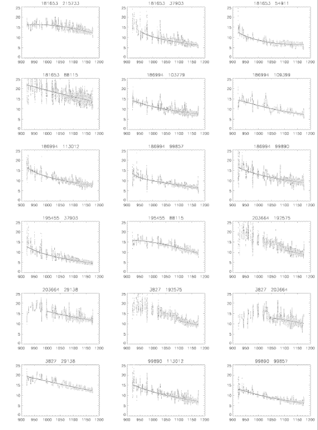
Figure 3: The extinction curves ($E(\lambda-V)/E(B-V)$ vs. wavelength in Å ) derived from 18 individual star pairs. The solid line is the smooth extinction curve derived from these data over the valid range.

For each of the star pairs listed in Table 2, we first correct the lightly-reddened star using the extinction curve of Cardelli, Clayton & Mathis (1989) extrapolated to 920 Å by fitting second order polynomial to their curve between 1250 and 1700 Å. (The Cardelli, Clayton & Mathis curve is formulated to agree with the Savage & Mathis (1979) curve for R${}_{v}=3.1.$) We then divide the two stellar spectra, discarding obviously outlying points and perform a least-squares fit to the ratio with a polynomial of order 2 – 4. The exact order selected by eye to provide a good characterization of the flux ratio. We then use this curve to arrive at an extinction curve for the pair via Eqn 1. In doing so, we apply a normalization factor of 0.9 to the spectra taken during ORFEUS I, on the recommendation of Hurwitz et al. (1998) for flux agreement with ORFEUS II. The data, flux ratio and fit for the pair of stars HD 186994 and HD 113012 are shown in Figs. 1 and 2. The gaps in the data in Fig. 2 are regions of the spectrum excluded because of H₂ absorption, but the continuum is still well characterized down to 920 Å. We performed each fit individually and present the range of validity in Table 2. The individual extinction curves and the curve fit in the valid range are shown in Fig. 3.

3 DISCUSSION

We show in Fig. 4 the extinction curves derived from all 18 star pairs, together with an extrapolation of the extinction curve (dashed line) of Savage & Mathis (1979). The extrapolation of the Savage & Mathis curve is done by a second order polymomial fit to their standard curve between 2000 and 1000 Å. The measured curves show significant scatter and we investigate here whether these differences arise from real variations in the extinction or from measurement uncertainties.

3.1 Uncertainties in the Measurement

A number of potential sources for uncertainty are discussed by Massa, Savage & Fitzpatrick (1983) and Cardelli, Sembach & Mathis (1992), who find that the three main sources of systematic error are stellar mismatch, the effects of an undiscovered stellar companion, and an improper deredding of the standard star. The formal uncertainties for each of the curves shown in Fig. 4 depend on the uncertainties in the quantities in Eqn. 1, which depend in part on these sources of systematic error. By evaluating the size of the uncertainties for the quantities in Eqn. 1, we can then estimate the uncertainty for a particular extinction curve. We use this information to determine the reliability of a particular curve and then decide whether or not to include it in our average. This procedure does not specifically evaluate wavelength-dependent effects in the uncertainties or analysis, as discussed by Massa, Savage & Fitzpatrick (1983). However, with the exception of the standard star reddening correction discussed below, the effect to the average curve from uncertainties with random sign is that these uncertainties become random and their effect on the average curve is estimated accordingly.

We have reasonable confidence in our stellar spectral classifications; the uncertainties of 0.3 in spectral type and half a luminosity class primarly enter into the uncertainty in $E(B-V)$. We estimate the likelihood of significant flux contamination from an unknown stellar companion to be small at these wavelengths; the companion would have to be of the rare early-B type or earlier to affect significantly the total flux from our sample stars.

An expression for the total uncertainty in an extinction curve is derived in the appendix. We use this formula to estimate the uncertainty for each extinction curve. We find that even this first-order estimate of the uncertainty provides a useful measure of the quality of the extinction curve derived from a given star pair. The uncertainties in $V$ and $B-V$, taken from the GCPD, average 0.014 and 0.009, respectively, for our program stars. The uncertainty in $E(B-V)$ is calculated to be 0.022, based on these uncertainties and the uncertainty in our spectral identifications. We show in Table 3 our estimates of the uncertainties in each quantity and their average contribution to the overall uncertainty in $E(\lambda-V)/E(B-V)$. The latter value is the difference between calculating the uncertainty (the average of all stars) normally and that found when setting the uncertainty in the given parameter to zero. The most significant of the individual uncertainties are the elements of $E(B-V)$, namely $V$, $(B-V)$ (both taken from GCPD) and $(B-V)_{0}$, based on our spectral type and luminosity class determinations. The overall uncertainty for a given curves varies with the uncertainty in $E(B-V)$. Minor variations in $R_{v}$ are insignificant, as shown in Table 3.

The largest contribution to the uncertainty derives from the uncertainty in $E(B-V)$ for the standard star and next from the reddened star. The dependence on the standard star reddening arises from the large reddening correction that must be applied at these wavelengths, while that from the reddened star directly affects the normalization of the extinction curve. We find that the uncertainty in the extinction curved derived for a pair of stars is anti-correlated with the reddening of the reddened star as shown in Fig. 5. This can be understood because the uncertainties in the stellar magnitudes are essentially independent of the reddening and are similar for each star. Thus the fractional uncertainty in the reddening of a star is greatest at low reddening, leading to a larger uncertainty in the final extinction curve. The effect of the $E(B-V)$ uncertainty is most significant in the highly-extincted FUV wavelengths measured here and represents a fundamental limitation on the use of the pair method at FUV wavelengths. An accurate measurement requires a well-reddened star, which in turn implies faint fluxes in the FUV region, a challenge for current instrumentation. At the longer wavelengths studied by Massa, Savage & Fitzpatrick (1983) using IUE data, it was possible to measure reddened stars having $E(B-V)$ as high as 1.21, leading to lower overall uncertainties.

The uncertainties we calculate for the individual extinction curves derived from each pair (for reference wavelength 1050 Å) are shown in Table 2. We show in Figure 6 those curves with uncertainty in $E(\lambda-V)/E(B-V)$ less than 1.7 and note that the variance is much reduced and the average appears close to the Savage & Mathis (1979) curve. It appears critical, then, that an evaluation of the uncertainty in an extinction curve be made before an assessment of whether the extinction curve appears anomalously high or low. Extinction curves in our sample derived from pairs of stars with reddening similar to those of Green et al. (1992) have uncertainties of about 1 calculated using our $E(B-V)$ uncertainty of 0.022 mag, but the uncertainty grows to greater than 20 mag in our error formulation if we match the $E(B-V)$ uncertainty of 0.5 magnitudes suggested in that paper. The anomalously low extinction of $\rho$ Oph is, however, confirmed by Fitzpatrick and Massa (1990). This caution is also relevant to an interpretation of the results of Buss et al. (1994), who in addition to the uncertainties discussed above must incur additional uncertainties by correcting for spectral type mismatch and comparing standard and reddened stars observed with different instruments. An excellent summary and discussion of peculiar extinction at longer UV wavelengths, including substantial attention to uncertainties, is given in Massa, Savage & Fitzpatrick (1983).

3.2 The New Measured Average Extinction Curve

We have averaged the 11 curves shown in Fig. 6 with a weighting inverse to their uncertainty to produce a mean extinction curve. To achieve uniform weighting of the seven reddened stars on which these curves were based, we also halved the weighting of each pair of curves that were derived from the same reddened star. We found the average curve was insensitive to whether we weighted each curve or each star equally, with the results agreeing to within 2%. The curve in Fig. 7 represents the mean extinction for the diffuse interstellar medium over the wavelength range 900 – 1200 Å, with the error bars indicating the uncertainty in the average based on the uncertainty in the individual measurements. The error bars range between 0.43 at the blue end to 0.35 at the red end. As many authors have discussed, intrinsic luminosity differences lead primarily to vertical displacements in the curve, rather than significant changes in its shape. Therefore, averaging several curves should yield a good approximation to the mean extinction. Curves that lie significantly outside of the uncertainty range of this mean curve may be said to be anomalous. Coefficients for a polynomial expression describing the mean curve in Figure 7 valid over the range 910 – 1200 Å are given in Table 4. If wavelength is in Angstroms, use the coefficients in the first column; if wavelength is in $\mu$m^-1 use the coefficients in the second column to calculate

$$\frac{E(\lambda-V)}{E(B-V)}=d_{0}+d_{1}x+d_{2}x^{2}$$ (2)

The upturn seen at shorter wavelengths in Figs. 6 and 7 appears to indicate a real steepening of the mean extinction curve below 1000 Å since it occurs coherently over many spectral bins for several stars. We show in Fig. 7 the Draine & Lee (1984, 1987) predictions using a grain-size distribution taken from Mathis, Rumpl & Nordieck (1977). This model agrees well with the curve above 1000 Å, but falls significantly below the average curve at shorter wavelengths, a finding also reported by Green et al (1992) and discussed therein. We note that though the standard star correction applied between 900 and 1000 Å is a pure extrapolation from longer wavelengths, the extrapolated extinction curve actually agrees very well with the final result, validating its use in our analysis. If instead the true extinction curve were as flat as the model suggests, this would have the effect of flattening the curves we derive. However, because the upturn appears in star pairs that have an extinction correction of less than a magnitude at 910 Å, this effect unable to explain the four-unit discrepancy between the mean curve and the model. We therefore infer that the upturn is real and it is the model that needs modification. More detailed modeling of the grain sizes and composition leading to the mean and individual extinction curves will appear in Paper II. The smooth behavior of the extinction curve between 1100 and 1200 Å does not seem to indicate an extinction bump like the 2175 Å feature, as suggested in Fitzpatrick & Massa (1988).

We note that our data processing makes our final result highly insensitive to small-scale ($<40$ Å) features in the extinction curve, if any are present. We also note that the distance to stars in this study ranges from approximately 0.8 to 6.6 kpc. Thus the dust producing the extinction comes from a range of environmental conditions and the net effect is an average of all the dust along the line of sight. We examined the 100$\mu$m dust emission maps of Schlegel et al. (1998) for any indications of unusual concentrations or peculiar dust absorption along the sightlines of the stars used in this study. Stars HD 97991 and HD 195455 were the only ones that were located in regions of significant dust emission. These two stars both have very low reddening and are used as standard stars in this study. This test raised no concerns about peculiar dust properties along the sightlines to our reddened stars. We also note the excellent agreement with the Cardelli, Clayton & Mathis (1989) curve for $R_{v}=3.1$ in the region of wavelength overlap. Hence our average curve may be regarded as typical for the diffuse ISM where an average value for $R_{v}=3.1$ is appropriate.

To examine how differences in luminosity class between the standard and reddened star affect the resulting extinction curve, we derived an average extinction curve after eliminating those three star pairs with luminosity differences of two or more luminosity classes. This resulting curve was slightly higher, by less than 2% everywhere, the change being smaller than the uncertainty shown for the average curve in Fig. 7. Two of the curves lie below the average curve while one lies above it, with the change to the average curve primarily arising because the lowest curve in Fig. 6 was eliminated. We are hesitant to draw significant conclusions about the effects of luminosity differences on the extinction curve in this wavelength range based on a sample of three pairs, but do note that the effect of their inclusion in the average curve is not large. Cardelli, Sembach & Mathis (1992) estimate uncertainties resulting from extreme luminosity-class differences in the wavelength range 1200 - 3200 Å. They find that noticeable differences in an extinction curve can arise when luminosity mismatch is extreme. However, they also find that this effect, though detectable, does not exceed the overall uncertainty in the derived extinction curve in that wavelength region.

4 CONCLUSIONS

We have made a new measurement of the FUV dust extinction curve in the Galactic diffuse interstellar medium from 910 to 1200 Å, using high resolution data from the ORFEUS telescope of a carefully selected sub-sample of B stars and a new model for H₂ absorption. This work is the first detailed study of extinction in this wavelength range using ORFEUS data and the comparatively large sample of stars we have available provides a substantially more reliable measurement than was previously available. We find good agreement between the average of our new measurements and an extrapolation from longer wavelengths of the standard curve of Savage & Mathis (1979), but find considerable individual variations among individual stellar pairs. We have shown that measurements of an individual FUV extinction curve are subject to large uncertainties arising primarily from the $E(B-V)$ values adopted for both the standard and reddened star. It is clear that credible claims of anomalous extinction curves at FUV wavelengths must be accompanied by a careful examination of the uncertainties in the quantities used to derive them.

Appendix A FORMULATION OF THE UNCERTAINTY

The standard-star correction function, $c(\lambda)$, in Eqn. 1,

$$E(\lambda-V)=-2.5\log\left(\frac{F_{red}(\lambda)}{c(\lambda)F_{st}(\lambda)}\right)+(V_{st}-E(B-V)_{st}R_{v}-V_{red}),$$ (A1)

can be rewritten in terms of $A_{\lambda}$ for the standard star. We calculate $A_{\lambda,st}$ from

$$A_{\lambda,st}=E(B-V)_{st}\left(\frac{E(\lambda-V)}{E(B-V)}+R_{v}\right).$$ (A2)

The uncertainty in the extinction curve may then be calculated from

$$\frac{E(\lambda-V)}{E(B-V)}=\frac{1}{E(B-V)_{red}}\left[-2.5\log\left(\frac{F_{red}}{F_{st}}\right)+A_{\lambda,st}-E(B-V)_{st}R_{v}+V_{st}-V_{red}\right].$$ (A3)

If we define X to be the term in brackets, the uncertainty in the extinction curve on the left side of Eqn. 5 can be written

$$\delta\left\{\frac{E(\lambda-V)}{E(B-V)}\right\}=\frac{1}{E(B-V)_{red}}\left[\left(\frac{X}{E(B-V)_{red}}\right)^{2}\sigma_{E(B-V)_{red}}^{2}+\sigma_{X}^{2}\right]^{1/2}.$$ (A4)

We can write $\sigma_{X}$ as

$$\sigma_{X}=\{\sigma_{\alpha}^{2}+\sigma_{\beta}^{2}+\sigma_{\delta}^{2}+\sigma_{V_{st}}^{2}+\sigma_{V_{red}}^{2}\}^{1/2},$$ (A5)

where

$$\sigma_{\alpha}=2.5\left[\left(\frac{\log_{10}e}{F_{st}}\right)^{2}\sigma_{F_{st}}^{2}+\left(\frac{\log_{10}e}{F_{red}}\right)^{2}\sigma_{F_{red}}^{2}\right]^{1/2},$$ (A6)

$$\sigma_{\beta}=\left\{\left(\frac{E(\lambda-V)}{E(B-V)}+R_{v}\right)^{2}\sigma_{E(B-V)_{st}}^{2}+\left(\sigma_{R_{v}}^{2}+\sigma_{\frac{E(\lambda-V)}{E(B-V)}}^{2}\right)E(B-V)_{st}^{2}\right\}^{1/2},$$ (A7)

and

$$\sigma_{\delta}=\left[E(B-V)_{st}^{2}\sigma_{R_{v}}^{2}+R_{v}^{2}\sigma^{2}_{E(B-V)_{st}}\right]^{1/2}.$$ (A8)

We use equation A4 to calculate the uncertainty of an individual extinction curve at a given wavelength.

Figure 1: The FUV spectra of HD 186994 (upper) and HD 113012 (lower) taken with the Berkeley spectrometer on the ORFEUS telescope. Significant H₂ absorption is evident in the both spectra; we model H₂ in the spectra and exclude regions of the spectrum that show significant absorption by H₂.

Figure 2: The ratio of the two spectra shown in Fig. 1 and the polynomial fit that characterizes the curve. Significant flux is detected in the two stars to 920 Å.

Figure 4: The extinction curves derived from the star pairs shown in Table 2. The dashed curve is from Savage & Mathis (1979). The scatter in these curves is due both to measurement uncertainties and intrinsic variations in the extinction.

Figure 5: The uncertainty in the extinction curves decreases when more heavily reddened stars are used, with a much weaker dependence on minor variations in the reddening of the standard star.

Figure 6: The extinction curves derived from the star pairs with the lowest uncertainties. The dashed curve is from Savage & Mathis (1979). Removing the curves with the highest uncertainty substantially reduces the variation in the sample.

Figure 7: The average extinction curve derived from the measurements with the lowest uncertainties. The dashed curve is from Savage & Mathis (1979); the dot-dashed curve is the Draine & Lee (1984, 1987) model discussed in the text. The error bars are derived from the uncertainties of the constituent curves at each wavelength shown.

Table 1: BASIC DATA ON PROGRAM STARS AND SPECTRAL TYPE RESULTS

Name	ORF	$l$	$b$	V	B-V	Spectral Type		$E(B-V)$	$(B-V)_{0}$	Ref.
HD	1/2	(deg)	(deg)	(mag)	(mag)	Published	This Work
3827	1	120.79	-23.23	8.01	-0.235	B0.7Vn	B0.5V	0.05	-0.28	DS94
29138	1	297.99	-30.54	7.19	-0.064	B1.0Iab	B0.2III/	0.20	-0.27	DS94
							B0.5Ib-II
37903	2	206.85	-16.54	7.83	0.103	B1.5V	B1.5V	0.35	-0.25	DS94
54911	1	229	-3.06	7.34	-0.082	B2.0II	B1III	0.18	-0.26	DS94
88115	1	285.32	-5.53	8.32	-0.053	B1.5IIn	B1Ib	0.14	-0.19	DS94
97991	2	262.34	51.73	7.40	-0.217	B2.0V	B1V	0.04	-0.26	DS94
99857	1	294.78	-4.94	7.47	0.125	B0.5Ib	B0II	0.41	-0.29	DS94
99890	1	291.75	4.43	8.30	-0.059	B0.0IIIn	B0III	0.24	-0.30	DS94
103779	2	296.85	-1.02	7.21	-0.002	B0.5Iab	B0III	0.30	-0.30	DS94
104705	1	297.45	-0.34	7.79	-0.011	B0Ib	B0II	0.28	-0.29	DS94
109399	1	301.71	-9.88	7.62	0.001	B0.7II	B0II-III	0.30	-0.30	DS94
113012	2	304.21	2.77	8.14	0.110	B0.2Ib	B0III-IV	0.41	-0.30	DS94
121800	2	113.01	49.76	9.11	-0.17	B1.5V	B2Ib	0.00	-0.16	DS94
181653	2	98.22	22.49	8.4	-0.20	B1II-III	…	0.05	-0.25	W71
186994	2	78.62	10.06	7.50	-0.129	B0III	B0III-IV	0.17	-0.30	HL77
192575	2	101.44	18.15	6.83	0.166	B0.5V	…	0.45	-0.28	C86
195455	1	20.27	-32.14	9.20	-0.18	B0.5III	B1II	0.06	-0.24	DS94
203664	2	61.93	-27.46	8.57	-0.20	B0.5V	…	0.08	-0.28	F94
215733	2	85.16	-36.35	7.33	-0.135	B1II	B1II	0.11	-0.24	F94
217505	1	325.53	-52.6	9.14	-0.208	B2III	B2.5IV	0.00	-0.22	KBL86
219188	2	83.03	-50.17	7.0	-0.20	B0.5III	B0.5II	0.08	-0.28	F94
233622	1	168.17	44.23	10.01	-0.21	B2V	B2.5II	0.00	-0.19	R97

Note. — Mean $V$ and B Vcolors are taken from the General Catalog of Photometric Data by Mermilliod et al. 1997. Published spectral types key:

DS94 – Diplas & Savage (1994), W71 – Walborn (1971), HL77 – Hill & Lynas-Gray (1977), C86 – Carnochan (1986), F94 – Fruscione et al. (1994), KBL86 – Keenan et al. (1986), R97 – Ryans et al. (1997)

Table 2: STAR PAIRS, FIT PARAMETERS, AND UNCERTAINTY

Reddened Star	Standard Star	Spectral Type		$\Delta E(B-V)$	Range Fit	Order of fit	Uncertainty
HD	HD	Reddened	Standard		(Å)		$\frac{E(\lambda-V)}{E(B-V)}$
29138	3827	B0.2III/B0.5Ib-II	B0.5V	0.15	920-1180	3	2.02
29138	203664	B0.2III/B0.5Ib-II	B0.5V	0.12	980-1180	3	2.07
37903	195455	B1.5V	B1II	0.29	920-1180	3	0.98
37903	181653	B1.5V	B1II-III	0.30	1040-1180	2	1.04
54911	181653	B1III	B1II-III	0.13	920-1180	3	2.56
88115	195455	B1Ib	B1II	0.08	920-1180	3	2.59
88115	181653	B1Ib	B1II-III	0.09	920-1180	3	3.00
99857	186994	B0II	B0III-IV	0.24	920-1180	4	0.85
99857	99890	B0II	B0III	0.17	920-1180	3	0.92
99890	186994	B0III	B0III-IV	0.07	920-1180	3	1.69
103779	186994	B0III	B0III-IV	0.13	920-1180	4	1.45
109399	186994	B0II-III	B0III-IV	0.13	920-1180	4	1.41
113012	99890	B0III-IV	B0III	0.17	920-1180	3	1.17
113012	186994	B0III-IV	B0III-IV	0.24	920-1180	3	1.09
192575	3827	B0.5V	B0.5V	0.40	1060-1180	4	0.97
192575	203664	B0.5V	B0.5V	0.37	1060-1180	3	0.99
203664	3827	B0.5V	B0.5V	0.03	1050-1180	2	4.18
215733	181653	B1II	B1II-III	0.06	920-1180	3	4.50

Note. — $\Delta E(B-V)$ is the difference in reddening between the standard and reddened star.

Table 3:

UNCERTAINTIES
Quantity	Typical Uncertainty	Relative Contribution to Uncertainty
	Used	in $E(\lambda-V)/E(B-V)$
$E(B-V)_{st}$: (total, mag)	0.02	1.0
$(B-V)_{o}$	0.02	…
B-V	0.009	…
$E(B-V)_{red}$: (total, mag)	0.022	0.75
$E(\lambda-V)/E(B-V)$:	1.0	0.1
$F_{st}$	5%	0.02
$F_{red}$	5%	0.02
$V_{st}$ mag	0.014	0.002
$V_{red}$ mag	0.014	0.002
$R_{v}$	0.2	0.008

Table 4: FIT COEFFICIENTS FOR FUV EXTINCTION CURVE

$d_{i}~{}~{}~{}$	$x=\lambda$(Å)	$x=\lambda^{-1}$ ($\mu m^{-1}$)
$d_{0}~{}~{}~{}$	116.176	34.7847
$d_{1}~{}~{}~{}$	-0.177494	-7.92908
$d_{2}~{}~{}~{}$	7.23734e-05	0.555443

References

- (1) Buss, R. H., Allen, M., McCandliss, S., Kruk, J., Liu, J. -C. & Brown, T., 1994, Ap.J., 430, 630
- (2) Cardelli, J. A., Clayton, G. C., & Mathis, J. S., 1989, Ap. J., 345, 245
- (3) Cardelli, J. A., Sembach, K., & Mathis, J. S., 1992, A. J., 104, 1916
- (4) Carnochan, D. J. 1986, MNRAS, 219, 903
- (5) Colangeli, L., Mennella, V., Palumbo, P., Rotundi, A., & Bussoletti, E., 1995, A&AS, 113, 561
- (6) Diplas, A. & Savage, B. D. 1994, ApJS, 93, 211
- (7) Dixon, W. V., Lee, D.H., & Hurwitz, M., 2001, Ap. J., submitted
- (8) Dixon, W. V., Hurwitz, M., & Bowyer, S., 1998, Ap. J., 492, 569
- (9) Draine, B.T. & Lee, H. M., 1984, ApJ, 285, 89
- (10) Draine, B.T. & Lee, H. M., 1987, ApJ, 318, 485
- (11) Fitzgerald, T., 1970, A& A, 4, 234
- (12) Fitzpatrick, E. L. & Massa, D., 1986, Ap. J., 307, 286
- (13) Fitzpatrick, E. L. & Massa, D., 1988, Ap. J., 328, 734
- (14) Fitzpatrick, E. L., 1989, in IAU 135: Interstellar Dust, Kluwer Academic Publishers, Boston, p. 37
- (15) Fitzpatrick, E. L. & Massa, D., 1990, ApJS., 72, 163
- (16) Fruscione, A., Hawkins, I., Jelinsky, P., & Wiercigroch, A. 1994, ApJS, 94, 127
- (17) Green, J., Snow, T. P., Cook, T. A., Cash, W. C., & Poplawski, O., 1992, Ap. J., 395, 289
- (18) Gordon, K. D. & Clayton, G. C., 1998, Ap. J., 500, 816
- (19) Hill, P.W & Lynas-Gray, A.E., 1977, MNRAS, 180, 691
- (20) Hurwitz, M. et al., 1998, Ap. J. Letters, 500, L1
- (21) Keenan, F. P., Brown, P. J. F., & Lennon, D. J. 1986, A&A, 155, 333
- (22) Longo, R., Stalio, R., Polidan, R. S. & Rossi, L., 1989, Ap. J., 339, 474.
- (23) Massa D, Savage, B. D. & Fitzpatrick, E. L., 1983, Ap. J., 266, 662
- (24) Mathis, J. S. & Cardelli, J. A., 1992, Ap. J., 398, 610
- (25) Mathis, J. S., Rumpl, W. & Nordsieck, K. H., 1977, Ap. J., 217, 425
- (26) Mermilliod, J.-C., Mermilliod, M. & Hauck, B., 1997, A & A Supp., 124, 349 (GCPD)
- (27) Mihalas, D., & Binney, J., 1981, Galactic Astronomy (W.H. Freeman & Co., San Francisco)
- (28) Misselt, K. A., Clayton, G. C., Gordon, K. D., 1999, Ap. J., 515, 128
- (29) Morton, D. C., 1978, Ap. J., 222, 863.
- (30) Puget, J. L. & Léger, A., 1989, ARA&A, 27, 161
- (31) Rountree, J. & Sonneborn, G., 1993, NASA Ref. Pub. 1312
- (32) Rountree, J. & Sonneborn, G., 1991, Ap. J., 369, 515
- (33) Ryans, R. S. I., Keenan, F. P., Sembach, K. R., & Davies, R. D. 1997, MNRAS, 289, 986
- (34) Sasseen, T. P., Hurwitz, M., Dixon, W. V., & Bowyer, S., 1996, AAS, 188, 702
- (35) Savage, B.D. & Mathis, J., 1979, ARA&A, 17, 73
- (36) Schlegel, D., Finkbeiner, D., & Davis, M., 1998, Ap. J., 500, 525
- (37) Snow, T. P., Allen, M. M. & Polidan, R. S., 1990, Ap. J., 359, 23
- (38) Walborn, N., 1971, Ap. J. Supp., 23, 257
- (39) Weingartner, J. C. & Draine, B. T., 2001, Ap. J., 548, 296