Measuring the Redshift Evolution of Clustering: the Hubble Deep Field South

Abstract

We present an analysis of the evolution of galaxy clustering in the redshift interval $0\leq z\leq 4.5$ in the HDF-South. The HST optical data are combined with infrared ISAAC/VLT observations, and photometric redshifts are used for all the galaxies brighter than $I_{AB}\leq 27.5$. The clustering signal is obtained in different redshift bins using two different approaches: a standard one, which uses the best redshift estimate of each object, and a second one, which takes into account the redshift probability function of each object. This second method makes it possible to improve the information in the redshift intervals where contamination from objects with insecure redshifts is important. With both methods, we find that the clustering strength up to $z\simeq 3.5$ in the HDF-South is consistent with the previous results in the HDF-North. While at redshift lower than $z\sim 1$ the HDF galaxy population is un/anti-biased ($b\leq 1$) with respect to the underlying dark matter, at high redshift the bias increases up to $b(z\sim 3)\simeq 2-3$, depending on the cosmological model. These results support previous claims that, at high redshift, galaxies are preferentially located in massive haloes, as predicted by the biased galaxy formation scenario. In order to quantify the impact of cosmic errors on our analyses, we have used analytical expressions from Bernstein (1994). Once the behaviour of higher-order moments is assumed, our results show that errors in the clustering measurements in the HDF surveys are indeed dominated by pure shot-noise in most regimes, as assumed in our analysis. We also show that future observations with instruments like the Advanced Camera on HST will improve the signal-to-noise ratio by at least a factor of two; as a consequence, more detailed analyses of the errors will be required. In fact, pure shot-noise will give a smaller contribution with respect to other sources of errors, such as finite volume effects or non-Poissonian discreteness effects.

1 Introduction

It is well known that the evolution of the dark matter clustering can be reliably used to put strong constraints on cosmological models. In fact the growth of density fluctuations depends on the main cosmological parameters, namely the contribution of matter and cosmological constant to the present total energy density ($\Omega_{\rm 0m}$ and $\Omega_{\rm 0\Lambda}$, respectively). This result, confirmed by high-resolution N-body simulations (e.g. Jenkins et al. 1998), has been used to build a semi-empirical model which suitably relates the linear perturbation scale to the final non-linear scale of the same perturbation after collapse (Hamilton et al. 1991). This technique can be used to compute analytically the evolved correlation function starting from a given primordial density power-spectrum (e.g. Peacock & Dodds 1994, 1996; Jain, Mo & White 1995).

However, the application of this idea to real data is greatly complicated by the fact that the observed objects (galaxies, quasars, clusters, etc.) are not direct tracers of the dark matter distribution. Usually, the ignorance about the relation between the object density, $\delta_{\rm o}$, and the dark matter one, $\delta_{\rm m}$, is parametrized introducing the so-called bias parameter $b$, for which a simple linear relation is a common assumption: $b=\delta_{\rm o}/\delta_{\rm m}$ (Kaiser 1984). Note that this relation includes the details of structure formation and, as a consequence, is quite uncertain.

A possible shortcut to the solution of this problem is to relate the value of $b$ to some intrinsic property. For example, analytical models (e.g. Mo & White 1996; Catelan et al. 1998; Jing 1999; Sheth & Tormen 1999; Sheth, Mo & Tormen 2001), confirmed by the results of N-body simulations, suggest that the bias factor of dark matter haloes is a function only of their mass and formation redshift (apart from the cosmological parameters). If there is a way to relate a typical observational quantity of the considered objects (such as flux or luminosity) directly to the mass of their hosting dark matter haloes, the study of the clustering evolution fully recovers its ability to discriminate between different cosmological models. For instance, in the case of galaxy clusters detected in the X-ray band, the flux at a given redshift corresponds to a given halo mass, under the assumptions of virial isothermal gas distribution and spherical collapse. Hydrodynamical simulations confirm the resulting relations between mass and luminosity or temperature, even if with a large scatter. Then the comparison of the observed cluster two-point correlation function to theoretical predictions can be used to put some constraints to the cosmological parameters. For example, Moscardini et al. (2000a,b) find that the clustering properties of the clusters observed in different samples (RASS1 Bright Sample, XBACs, BCS and REFLEX) favour cosmological models with a low value of $\Omega_{\rm 0m}$.

In the case of galaxies, applying a similar technique is much more difficult, mainly because the relation between mass and luminosity is not one-to-one. Moreover, it is not clear how many galaxies can occupy a single halo of a given mass. However, once a cosmological framework is fixed, the study of the clustering evolution of galaxies can be used to obtain more information about the nature of these objects. For example, it is possible to estimate a typical value for the mass of the dark matter haloes hosting the galaxies. Moreover the clustering data can be used to discuss if the merging process is important at various redshifts or if the galaxy number tends to be conserved during the evolution. In fact, these two opposite models predict a completely different redshift evolution of the bias factor (see e.g. Matarrese et al. 1997 and Moscardini et al. 1998).

From the point of view of the observational data required for this kind of study, enormous progress has been made in recent years. Large spectroscopic surveys gave an accurate description of the spatial distribution of the galaxies in the local Universe. Statistical analyses have shown that the correlation length depends on morphological type and/or absolute magnitude: more luminous and/or early-type galaxies appear to have higher clustering than faint and/or late-type galaxies (Santiago & da Costa 1990; Loveday et al. 1995; Benoist et al. 1996; Norberg et al., 2001). However, these local observations can be reasonably well reproduced by a large variety of sensible cosmological models, while possible differences are expected at higher redshifts, as previously discussed. This has been one of the main reasons which motivated the extension of spectroscopic surveys to high redshifts. Nowadays, different samples are available to estimate the clustering properties of galaxies up to $z\approx 1$ [Canada-France Redshift survey (Le Fèvre et al. 1996); Hawaii K survey (Carlberg et al. 1997); Norris Redshift Survey (Small et al. 1999); Caltech Faint Redshift survey (Hogg, Cohen & Blandford 2000); Canadian Network for Observational Cosmology field galaxy redshift survey (Carlberg et al. 2000)]. Even if the sampled regions are relatively small, the results are in good agreement in showing a decline of the correlation length with redshift.

Up to a few years ago, clustering studies at higher redshifts were limited to peculiar objects like radiogalaxies or quasars. The discovery of reliable colour techniques (U-dropouts) made it possible to identify a large sample of ‘normal’ galaxies at $z\approx 3$, the so-called Lyman-Break galaxies (LBGs). By measuring the correlation function or computing the count-in cell statistics, different works (Adelberger et al. 1998; Giavalisco et al. 1998; Giavalisco & Dickinson 2000) showed that LBGs have a correlation length at least comparable with that of present-day spiral galaxies. This result corresponds to quite a high value for the bias factor at $z\sim 3$, suggesting that their formation occurs in massive dark-matter haloes.

An alternative way to probe larger volumes and/or fainter galaxy populations makes use of the photometric redshift technique (e.g. Lanzetta, Yahil & Fernández-Soto 1996; Sawicki, Lin & Yee 1997; Arnouts et al. 1999, hereafter A99; Bolzonella, Miralles & Pellò 2000). This method, based on the comparison of theoretical and/or real spectra with the observed galaxy colours in different bands, makes it possible to estimate their redshifts at higher magnitudes than those reached spectroscopically by the largest available telescopes. This is done in a probabilistic way; as a consequence, the estimates are affected by errors, which typically have been found to increase with redshift. Note that to date, these inherent uncertainties in the redshift estimates were completely ignored or estimated via simulations and used as an a posteriori global correction to the correlation measurements (A99). A more correct approach would require the estimate of the redshift uncertainty for each object and the inclusion of this information in the computation of the correlation function, as discussed in this paper.

Thanks to the application of the technique of photometric redshifts to its very deep observations, the Hubble Deep Field (HDF) North (Williams et al. 1996) has become a test case for the evolution of the galaxy distribution. The data of more than one thousand objects down to $I_{AB}\approx 28.5$ have been used to study the redshift evolution of the clustering up to $z\sim 4.5$ (A99; Magliocchetti & Maddox 1999; Roukema et al. 1999; see also the analysis made by Connolly, Szalay & Brunner 1998 up to $z\sim 1.2$). The results show that the comoving correlation length, after a small decrease in the interval $0\raise-2.0pt\hbox{\hbox to0.0pt{\hbox{$\sim$}\hss}\raise 5.0pt\hbox{$<$}\ }z\raise-2.0pt\hbox{\hbox to0.0pt{\hbox{$\sim$}\hss}\raise 5.0pt\hbox{$<$}\ }1$, increases up to $z\sim 4$. It is worthwhile to stress that the term “evolution” has not to be taken literally. Given a survey defined by its characteristic limiting magnitude and surface brightness, the galaxies observed at high $z$ typically have higher luminosities. Therefore, the intrinsic differences of the galaxy properties at different $z$ can mimic an evolution, i.e. the evolution measured in a flux-limited survey is not only due to the evolution of a unique population but can be due to a change of the considered population. In fact the theoretical modelling of the HDF galaxies shows that to reproduce their clustering properties at different redshifts, the mean mass of dark matter haloes hosting the galaxies is required to increase with $z$ (A99).

The reliability of the previous results, however, can be affected by the smallness of the observed field. In particular, it is not clear to what extent a region of a few square arcminutes can be considered representative of the properties of the whole Universe. The data more recently obtained in the HDF-South (Casertano 2000) offer a unique opportunity to test the robustness of HDF-North results, due to their mutual independence. For example, the field-to-field variations can be used to estimate the size of the cosmic variance on these scales. The main goal of this paper is to study in detail the clustering properties of HDF-South and to compare them with those obtained for the northern field to confirm or disprove the general picture described above.

The paper is organized as follows: In Section 2 we present the photometric database used in this analysis and briefly describe the photometric redshift technique. In Section 3 we introduce the two methods used to estimate the angular correlation function: the standard approach and an alternative method taking into account the photometric redshift uncertainties. Still in Section 3 we present the results of this analysis and estimate the bias factor. Section 4 is devoted to a theoretical discussion of the cosmic errors in the clustering estimates in Hubble Deep Fields. Conclusions are presented in Section 6.

2 The catalogue and photometric redshifts

2.1 The data

Deep high-resolution optical dataset ($F_{300}$, $F_{450}$, $F_{606}$ and $F_{814}$) from HST and deep infrared observations have been combined. The IR observations have been carried out in $J_{s},H,K_{s}$ passbands with the ISAAC instrument on the VLT (UT2) during the period July-September 1999. The total integration times are 7h, 6h and 8h in $J$, $H$ and $K_{s}$, respectively. The final coadded images have a seeing of 0.6 arcsec in $J_{s}$,$H$,$K_{s}$. The Vega magnitude limits in $2FWHMs$ at 5$\sigma$ level are 24,23,22.5 in $J_{s}$,$H$,$K_{s}$, respectively (Saracco et al. 2001).

The photometric catalogue containing the optical and infrared colours is described in detail in Vanzella et al. (2001). We recall here that the detections are based on the summed $V+I$ images and the deblending process has been tuned and optimized in order to obtain a photometric catalogue particularly reliable for photometric redshifts. Indeed a modified version of the SExtractor software (Bertin & Arnouts 1996) has been applied to optimize the SExtractor parameters (namely deblend-mincont, detect-minarea) in different regions of the frame. This procedure allows to improve the deblending of close pairs as well as to keep in single units large spiral galaxies and affects only the very small angular scales ($\theta\leq 3arcsec$). A catalogue of 1474 sources has been extracted up to $I_{AB}\simeq 28.5$.

2.2 The photometric redshift measurement

The technique of photometric redshifts adopted in this paper has been described in more detail in A99. The technique is based on $\chi^{2}$ minimisation which compares the observed magnitudes to the GISSEL96 synthetic library (Bruzual & Charlot 1993). In order to quantify the redshift uncertainties, in Figure1 we compare, for galaxies accessible to spectroscopy, the spectroscopic redshifts and those obtained using the photometric technique. The HDF-North sample is based on the list of Cohen et al. (2000) which is composed of 146 spectra. The HDF-South sample is based on 22 spectra from the list of Cristiani et al. (1999) observed with the VLT telescope and from Dennefeld et al. (2001) observed with NTT telescope. We also add 2 spectra observed with the Anglo Australian Telescope (Glazebrook et al., 1998). In the area of WFPC2 the HDF-South sample consists of 24 spectra, two of which are at $z_{\rm spec}>1.5$. The redshift accuracy is defined as in Fernández-Soto, Lanzetta & Yahil (1999): $(z_{\rm spec}-z_{\rm phot})/(1+z_{\rm spec})$, from which we extract the mean ($\Delta z$) and the dispersion ($\sigma_{z}$) by using a $\sigma$-clipping algorithm at $3\sigma$ rejection level. We obtain $\sigma_{z}=0.05$ and $\Delta z=0.03$ for $z_{\rm spec}\leq 1.5$ and $\sigma_{z}=0.05$ and $\Delta z=0.02$ for $z_{\rm spec}\geq 1.5$. Two catastrophic redshifts were initially rejected from the statistics (shown by large open squares in Figure 1) and six objects at $z\leq 1.5$ and two objects at $z\geq 1.5$ were rejected during the $\sigma$-clipping process (open circles in Figure 1). The total number of rejected objects is 10/170, corresponding to 6 per cent.

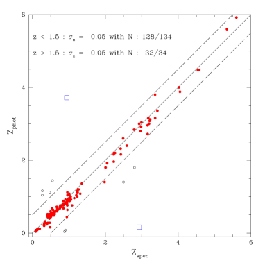
Figure 1: Dispersion between the spectroscopic redshifts and photometric estimates in the HDF-North (146 spectra) and HDF-South (24 spectra) (see text). The redshift dispersion ($\sigma_{z}$) is obtained by using a $3\sigma$-clipping rejection for two samples: z$\leq 1.5$ and $z\geq 1.5$. Catastrophic redshifts (represented by square symbols) have not been used in the measurement. Rejected objects during the $\sigma$-clipping are shown with open circle symbols. The solid line corresponds to $\Delta z=0$ and the long-dashed lines to $\Delta z=0.5$.

In Figure 2 we compare the redshift distributions obtained for the HDF-North and HDF-South for two intervals of magnitude, $I_{AB}\leq 26$ and $26\leq I_{AB}\leq 27.5$ (upper and lower panels, respectively). The two redshift distributions are similar. The Kolmogorov-Smirnov (KS) two-tail statistics does not reject the null hypothesis that the redshift distributions in the HDF-North and South are drawn from the same parent population. The KS-probability of the null hypothesis turns out to be 0.12 and 0.20 for the samples with $I_{AB}\leq 26$ and $26\leq I_{AB}\leq 27.5$ respectively. The median redshift in the HDF-North seems to be slightly higher for the bright sample, which is not surprising due to the presence of large-scale structures at $z\sim 1$ in the HDF-North (Cohen et al., 2000), also evidenced by systematic color differences (Vanzella et al., 2001).

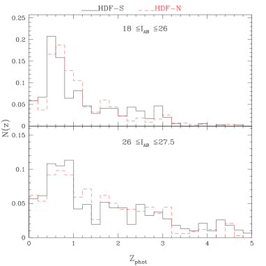
Figure 2: Comparison of the redshift distributions of the HDF-North (dashed line) and HDF-South (solid line) for galaxies brighter than $I_{AB}\leq 26$ (upper panel) and galaxies with magnitudes in the range $26\leq I_{AB}\leq 27.5$ (lower panel).

3 The angular correlation function

3.1 Selection of the sample

To compute the angular correlation function (ACF), we have limited our analysis to the region of the HDF-South with the highest signal-to-noise, excluding the area of the PC and the outer part of the three WFPC. The details of how the HDF-North and HDF-South photometric catalogues (Fernández-Soto et al. 1999; Vanzella et al. 2001) have been constructed are slightly different and the scale of the total $I$ magnitudes may present systematic differences. This is especially true at faint magnitudes. For this reason, rather than applying formally equal magnitude limits to the two samples, we prefer to adopt for HDF-South a limit that defines a roughly equal number of sources as in HDF-North and a comparable number of objects in each redshift interval (at least 100 except for the range $3.5\leq z\leq 4.5$). This can be accomplished by selecting in the HDF-South catalogue all galaxies brighter than $I_{AB}\simeq 27.5$. The total number of objects is 844 in an effective area of 4.45 $arcmin^{2}$. The nominal magnitude limit used in the HDF-North by A99 is $I_{AB}\simeq 28.5$ which provides 926 objects. Beyond $I_{AB}\sim 26$ the source counts in the HDF-S photometric catalog adopted in the present work are systematically higher than the corresponding counts in the HDF-North catalog used in A99 by a factor $\sim 1.5$. The discrepancy is to be ascribed to differences in the approach used to carry out the photometry in the two cases (Vanzella et al., 2001). The redshift bins used are the same as those adopted in the analysis of A99.

3.2 Classical ACF computation

The angular correlation function $\omega(\theta)$ is related to the excess of galaxy pairs in two solid angles separated by the angle $\theta$ with respect to a random distribution. The angular separation used for the computation of $\omega(\theta)$ covers the range from 3 arcsec up to 80 arcsec. We use logarithmic bins with steps of $\Delta\log(\theta)=0.3$. The lower limit of 3 arcsec is a conservative estimate of the scale over which we are confident about the deblending approach for resolved bright spirals or faint galaxy “groups”. The upper cut-off corresponds to almost half the size of the HDF regions and to the maximum separation where the ACF provides a reliable signal.

To derive the ACF in each redshift interval, we used the estimator defined by Landy & Szalay (1993, hereafter LS93):

$$\omega_{\rm est}(\theta)\ =\ A_{1}\ \frac{DD(\theta)}{RR(\theta)}-2A_{2}\ \frac{DR(\theta)}{RR(\theta)}+1\ ,$$ (1)

where DD is the number of different galaxy pairs, DR is the number of galaxy-random pairs and RR refers to random-random pairs with separation between $\theta$ and $\theta+\Delta\theta$. The normalisation factors $A_{1}$ and $A_{2}$ are given by

$$A_{1}=\frac{N_{r}(N_{r}-1)}{N_{g}(N_{g}-1)}\hbox{\ \ \ ;\ \ \ }A_{2}=\frac{N_{r}-1}{2\ N_{g}}\ ,$$ (2)

where $N_{g}$ and $N_{r}$ are the total number of objects in the data and random catalogues, respectively. In the present work the random catalogues contain $N_{r}=20000$ sources covering the same area as our HDF sample.

In the weak clustering limit, the above estimator has a nearly Poissonian variance (see LS93), so the uncertainty is estimated as:

$$d\omega_{\rm est}(\theta)=\sqrt{\frac{1+\omega_{\rm est}(\theta)}{<RR(\theta)>}}\hbox{\ \ \ ;\ \ \ }<RR(\theta)>=RR(\theta)/A_{1}$$ (3)

The results of our analysis will be discussed in Section 3.4, where they will be compared with those obtained by the alternative approach, described in the next subsection.

3.3 Alternative ACF method

3.3.1 Redshift probability distribution function

In our previous analysis of HDF-North (A99), we used Monte Carlo simulations to discuss the effects of uncertainties in the $z_{\rm phot}$ estimates on the clustering results. In particular we used the simulations to obtain the statistical errors in each redshift interval according to the limiting magnitude and to define an upper limit to the amplitude of the ACF assuming that the contamination effects are due to an uncorrelated population. In the present work, we define an alternative method which includes directly in the ACF measurement the redshift probability distribution of each object. For each object we measure a redshift probability distribution function (hereafter $PDFz$) estimated as follows:

$$PDFz\propto\exp\left(-\frac{\chi_{\rm min}^{2}(z)}{2}\right)\ \ \hbox{with}\ \ \chi^{2}_{\rm min}(z)=\sum_{i}\left[{F_{{\rm obs},i}-s\cdot F_{{\rm tem},i}(z)\over\sigma_{i}}\right]^{2}\ ,$$ (4)

where $\chi_{\rm min}^{2}(z)$ is the best fit value obtained at redshift $z$; $F_{{\rm obs},i}$ is the observed flux; $F_{{\rm tem},i}(z)$ is the template flux at redshift $z$ in $i$-th band, $\sigma_{i}$ is the photometric error in $i$-th band and $s$ is the scaling factor applied to the template fluxes as described in A99 (Equation 2). The $PDFz$ is then normalised to unity over the full range used to derive the redshift (here $0\leq z\leq 6$).

This $PDFz$ makes it possible to follow the redshift probability for each object (see also Bolzonella, Miralles & Pellò 2000) and has some similarity with the Bayesian photometric redshift estimation (Benítez 2000). To illustrate the behaviour of the $PDFz$, in Figure 3, (left panel) we show two examples for one object at $z_{\rm phot}=3.52$ with a secondary peak at $z_{\rm phot}=0.32$ (upper panel) and one at $z_{\rm phot}=2.56$ with no secondary peak (lower panel). In Figure 3 (right panel) we also compare the redshift distribution for objects brighter than $I_{AB}=27.5$ obtained by using the best redshift for the sources (solid line) and by summing the normalized $PDFz$ of all objects (dashed line). The spread in the individual $PDFz$ results in a sort of smoothing of the distribution obtained with the best redshift estimates.

Figure 3: Left panel: Two examples of redshift probability function for one object with a secondary redshift peak (upper panel) and for one object without secondary peak (lower panel). The area below the curves is normalised to unity. Right panel: Redshift distributions for galaxies with $I_{AB}\leq 27.5$ using the best redshift value for each object (solid line histogram) and by summing up the normalized $PDFz$ (dashed line histogram).

3.3.2 Weighted ACF measurement

In the previous section, we have computed the ACF assuming the best redshift value for each object regardless of its confidence level. In this section we take the redshift uncertainty into account directly in the ACF measurement by using the $PDFz$ of each object. For all the galaxies within a given redshift interval, we use the $PDFz$ to weight the number of pairs according to the probability of the objects being in the redshift bin. In Figure 4 we compare in the different redshift intervals the distribution obtained with the best redshift approach and that resulting from the summed $PDFz$ approach. The results are summarized in Table 1. We find that:

$1)$ The summed $PDFz$ are in general similar to the original distributions and have tails in the neighbouring intervals. The enlargement of the distribution corresponds to a change between 5 and 30 per cent. This effect is mainly due to the redshift uncertainties of objects at the boundaries of the bins under consideration.

$2)$ At redshifts between 0.5 and to 3.5, a very small fraction of objects shows catastrophic secondary redshifts ($\leq 5$ per cent). For the extreme bins the behaviour is different. The $3.5\leq z\leq 4.5$ bin shows a pronounced secondary peak at low $z$ corresponding to $13.5$ per cent of the total. The $0\leq z\leq 0.5$ redshift bin shows a long tail between $1\leq z\leq 4$ corresponding to a fraction of 31.5 per cent.

We find that the fraction of lost objects for different redshift ranges is in good agreement with the Monte Carlo simulations carried out in A99, where a gaussian random noise has been added to the original photometric errors (see Figure 4 of A99). This shows that the two approachs provide similar results to quantify the photometric redshift confidence levels.

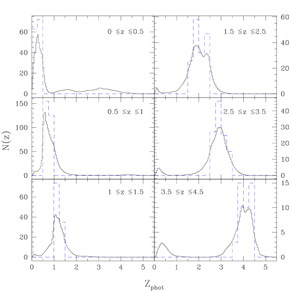
Figure 4: Histograms of photometric redshifts in different redshift bins (specified in each panel) defined by the best redshift (dashed lines) as compared with the histograms obtained for the same objects taking into account the redshift probability function (solid lines).

Table 1: Distribution of the $PDFz$ for different redshift intervals. Column 1: redshift bin. Column 2: fraction of objects within the redshift range. Column 3: fraction distributed in the adjacent bins. Column 4: fraction in non-adjacent bins.

$z$ range	Fraction in	Fraction in	Fraction in
	the bin (%)	adj. bins (%)	non adj. bins (%)
0.0 - 0.5	63	5.5	31.5
0.5 - 1.0	73.5	21.5	5
1.0 - 1.5	66	30	4
1.5 - 2.5	79	17	4
2.5 - 3.5	78.5	16.5	5
3.5 - 4.5	74.5	12	13.5

Since the ACF measurements in the HDFs is based on a small sample, we want to optimize the reliability of the signal in each redshift bin. The strategy adopted in the following analysis is to include in each redshift bin only the objects for which the best redshift belongs to the bin. We call $N_{\rm data}$ their number. This allows also a direct comparison between the classical ACF and this method.

To measure the weighted ACF, the number of pairs in the redshift range $z_{\rm min}\leq z\leq z_{\rm max}$, entering in equation 1, is replaced as follows:

$$DD\ =\ \sum_{i,j}^{N_{\rm data}}Pb^{i}\cdot Pb^{j}\hbox{\ ; \ }DR\ =\ \sum_{i=1,j=1}^{N_{\rm data},N_{r}}Pb^{i}\ ,$$ (5)

where $Pb^{i}$ represents the integral of $PDFz$ between $z_{\rm min}$ and $z_{\rm max}$ for the $i$-th object.

The normalisation factors $A_{1}$ and $A_{2}$ are the same except that the total number of objects $n_{D}$ is replaced by $n_{D}=\sum_{i=1}^{N_{\rm data}}Pb^{i}$.

The results are presented in the next subsection.

3.4 Results

In this section we discuss the clustering properties of the HDF-South. Figure 5 presents the measurements of the ACF in different redshift bins obtained using both methods discussed in the previous subsections. In particular, filled circles refer to the classical ACF estimates and open circles to the weighted ACF ones. Note that the errorbars are slightly larger for this last method. In fact, in this case the effective number of contributing points $n_{D}$ is smaller, as the galaxies have a non-vanishing probability outside their bin.

In order to give a more quantitative estimate of the correlation strength, we fit the data by adopting a power-law form for the ACF as $\omega(\theta)=A_{\omega}\theta^{-\delta}$. If the spatial correlation function $\xi$ is also assumed to follow a power-law relation, i.e. $\xi(r)=(r/r_{0})^{-\gamma}$, the slope $\gamma$ is simply related to $\delta$: $\gamma=\delta+1$. Since the galaxy samples are small, we prefer to derive the amplitude $A_{\omega}$ by fixing the value of $\delta$. As in A99, we adopt $\delta=0.8$ but we will discuss this assumption later.

Due to the small size of the considered field, we have to take into account the integral constraint $IC$ (Peebles 1974) in our fitting procedure as:

$$\omega_{\rm est}\simeq\omega_{\rm true}-IC\ .$$ (6)

The quantity $IC$ is defined as the integral of the ACF over the survey, i.e.

$$IC=\overline{\omega}_{\theta_{\rm max}}=\frac{1}{\Omega^{2}}\int\int\omega(\theta)d\Omega_{1}d\Omega_{2}=A_{\omega}\times B\ ,$$ (7)

where $\theta_{\rm max}$ is the maximum scale of the survey. The integral $B$ has been computed by a Monte-Carlo method using the same geometry as the HDF-South and masking the excluded regions. Adopting the value $\delta=0.8$, we derive $B=0.033$ (for $\theta$ measured in arcsec).

The fitting power-law relations are all shown in Figure 5, both for the classical ACF (solid lines) and weighted ACF (dashed lines), while the values of the amplitude of $\omega(\theta)$ at 10 arcsec are reported in Table 2. In general we find a good agreement between the results of the two different techniques. We find some differences only in the two extreme redshift bins ($\langle z\rangle=0.25$ and $\langle z\rangle=4$), where the objects typically display significant tails in the $PDFz$. Here the weighted ACF seems to allow a better extraction of the signal, giving larger values for the correlation function. However, due to the large errorbars, the two methods are still consistent at the $1\sigma$ level. Finally we note that in the redshift bin between $3.5\leq z\leq 4.5$ the results are consistent with the assumption of vanishing clustering.

Figure 5: The angular correlation functions $\omega(\theta)$ for galaxies with $I_{AB}\leq 27.5$ measured for different redshift intervals (as specified in each panel). The uncertainties are nearly Poisson errors. The results and the power-law best-fit obtained using the classical ACF estimator are shown by filled circles and solid lines, while open circles and dashed lines refer to the results obtained with the weighted ACF estimator.

In order to discuss the effects of the assumed slope on the clustering normalisation, in Table 2 we also show the amplitudes obtained using $\delta=0.6$ and $\delta=0.9$. The integral constraints $IC$ have been recomputed according to the slope: we find $B=0.074$ and $B=0.022$ for $\delta=0.6$ and $\delta=0.9$, respectively. The results show that the impact of the changes in the assumed slope affects the values of $A_{\omega}$ at 10 arcsec by less than $1\sigma$.

Table 2: The amplitude of $\omega(\theta)$ at 10 arcsec ($A_{\omega}$) for different redshift bins. Column 1: redshift interval. Column 2: number of galaxies with $I_{AB}\leq 27.5$ and best photometric redshift belonging to the redshift bin. Columns 3 and 5: amplitude $A_{\omega}$ computed assuming a slope $\delta=0.8$ for the classical and weighted ACF estimator, respectively. Column 4: amplitude $A_{\omega}$ computed using the classical ACF but assuming a different slope ($\delta=0.6$ and $\delta=0.9$).

		Classical ACF		Weighted ACF
$z$ range	Number	$A_{\omega}$(10arcsec)		$A_{\omega}$(10arcsec)
	$I_{AB}\leq 27.5$	$\delta=0.8$	$\delta=0.6,0.9$	$\delta=0.8$
0.0 - 0.5	135	0.07$\pm$0.05	0.07,0.07	0.13$\pm$0.08
0.5 - 1.0	281	0.06$\pm$0.02	0.07,0.06	0.05$\pm$0.04
1.0 - 1.5	109	0.10$\pm$0.06	0.12,0.09	0.12$\pm$0.09
1.5 - 2.5	163	0.08$\pm$0.04	0.09,0.08	0.06$\pm$0.05
2.5 - 3.5	113	0.16$\pm$0.05	0.19,0.15	0.21$\pm$0.08
3.5 - 4.5	43	0.01$\pm$0.15	0.03,0.00	0.09$\pm$0.23

It is important now to compare the clustering properties of HDF-South to the corresponding results for HDF-North that we obtained in our previous analysis (A99). The comparison is presented in Figure 6. The left panel shows the behaviour of $A_{\omega}$ computed at 10 arcsec (and multiplied by the bin size $\Delta z$, for consistency with A99). In spite of the smallness of the regions, the amplitudes of the correlation function measured in the two Hubble deep fields are in good agreement, showing a small field-to-field variation. The results confirm the behaviour of the clustering with the redshift we found in A99. Namely, the clustering amplitude declines from $z=0$ to $z\sim 1$ and increases at higher redshifts to become, at $z\geq 2$, comparable to or higher than that observed at $z\simeq 0.25$. At $z\simeq 4$ the clustering signal measured in HDF-South is very noisy and we cannot confirm the high value of $A_{\omega}$ found in the northern field. An alternative measure of the correlation strength is the comoving correlation length $r_{0}$. Its redshift evolution, computed, as in Magliocchetti & Maddox (1999), assuming a flat universe with present matter density parameter $\Omega_{\rm 0m}=0.3$, is shown in the right panel of Figure 6. Again, we find a slightly declining or almost constant behaviour up to $z\simeq 1$ and an increasing trend from $z\simeq 2$ to $z\simeq 3$.

Figure 6: Comparison of the clustering properties of galaxies in HDF-North and South. Left panel: the redshift evolution of the ACF amplitude $A_{\omega}$ at 10 arcsec (multiplied by the bin size $\Delta z$). Open triangles refer to the values of the HDF-North obtained by A99, while filled and open circles refer to the results obtained in this work adopting the classical and the weighted estimators, respectively. The different measurements have been shifted by $z=\langle z\rangle+/-0.05$ for clarity. Right panel: the redshift evolution of the comoving correlation length $r_{0}(z)$ (in $h^{-1}Mpc$) as computed by assuming a flat universe with $\Omega_{\rm 0m}=0.3$. The meaning of different symbols is the same as in the left panel.

Since the clustering amplitude of the dark matter decreases continuously with redshift (the actual behaviour depending on the cosmological scenario), the observed increase of the galaxy clustering at high redshift implies that galaxies at $z\approx 3-4$ are biased tracers of the underlying dark matter. This effect is illustrated in Figure 7, where we show the bias parameter $b$ as a function of redshift both for the HDF-South and HDF-North. The values of $b$ are computed by dividing the rms galaxy density fluctuation inside a sphere of $8h^{-1}Mpc$ at a given $z$ ($\sigma_{8}^{\rm gal}$) by the rms mass density fluctuation ($\sigma_{8}^{\rm m}$) predicted by linear theory. We consider two cosmological models with a cold dark matter ($CDM$) power spectrum normalised to reproduce the local cluster abundance (Eke, Cole & Frenk 1996): an Einstein-de Sitter $SCDM$ model ($\sigma_{8}^{m}(z=0)=0.52$ and $\Gamma=0.45$; left panel) and a flat $\Lambda CDM$ model with $\Omega_{\rm 0m}=0.3$ and $\Omega_{0\Lambda}=0.7$ ($\sigma_{8}^{m}(z=0)=0.93$ and $\Gamma=0.21$; right panel). The observed bias parameters for the HDF-South are in good agreement with our previous results for the northern field. In particular we observe some anti-bias ($b(z<1)\sim 0.5$) at low redshift, while we confirm that the high-redshift galaxies are strongly biased with respect to the dark matter: $b(z\sim 3)\sim 3,2$ for the $SCDM$ and $\Lambda CDM$ models, respectively. This supports a model of biased galaxy formation where $b$ is evolving with redshift. For comparison, in the same plot we also show the theoretical expectations for the effective bias (see Matarrese et al. 1997 and Moscardini et al. 1998 for a definition) computed for the same cosmological models using different minimum mass for the dark matter haloes ($M_{\rm min}=10^{10},10^{11},10^{12}h^{-1}M_{\odot}$). For the Einstein-de Sitter model, we can reproduce the observations with a minimum mass $M_{\rm min}\simeq 10^{10}h^{-1}M_{\odot}$ at $z\leq 1$ and $M_{\rm min}\simeq 10^{11}h^{-1}M_{\odot}$ between $1\leq z\leq 3$. For the $\Lambda CDM$ model $M_{\rm min}<10^{10}h^{-1}M_{\odot}$ is required at $z\leq 1$ , $10^{10}\leq M_{\rm min}\leq 10^{11}h^{-1}M_{\odot}$ for $1\leq z\leq 2$ and $M_{\rm min}\geq 10^{11}h^{-1}M_{\odot}$ at $<z>=3$ are required.

At redshift $z\simeq 3$, alternative estimates of the galaxy clustering come from the analysis of the Lyman Break Galaxy (LBG) samples. We find that the bias measured for the HDF-population is smaller than the one observed for the bright LBGs (Steidel et al. 1996). Assuming for example an Einstein-de Sitter model, Adelberger et al. (1998) found for the spectroscopic sample of LBGs a bias parameter $b(z=3)\approx 6$ while Giavalisco et al. (1998) found $b(z=3)\approx 4.5$ from the photometric sample (see also Giavalisco & Dickinson 2001). Averaging our results for HDF-South and HDF-North, we find $b(z=3)\approx 2.8$. These differences can be explained by the different surface galaxy densities (larger in the HDF fields, which have approximately 30 objects per square arcmin). In fact in the hierarchical galaxy formation scenario, more massive and rare objects form in rarer and higher peaks of the underlying matter density field; as a consequence they are expected to have a higher value of the bias parameter.

Figure 7: The measured bias $b$ as a function of redshift for an Einstein-de Sitter $SCDM$ model and $\Lambda CDM$ model (left and right panels). The open triangles refer to the values obtained for the HDF-North in A99; filled and open circles refer to the values obtained in this work for the HDF-South using the classical ACF and the weighted ACF estimators, respectively. The different lines represent the theoretical effective bias computed for the same cosmological models assuming different values of minimum mass $M_{\rm min}$. We show results for $M_{\rm min}=10^{10}$ (solid lines), $10^{11}$ (short-dashed lines) and $10^{12}$ (long-dashed lines) $h^{-1}M_{\odot}$.

4 The error budget

Up to now, we have assumed in our measurements that the errors are nearly Poissonian. We have neglected other possible contributions to the errors, due to the finite area of the survey or to the clustered nature of the galaxy distribution. In this section we deal with these effects basing our analysis on analytical expressions of the cosmic errors calculated by Bernstein (1994). We estimate the relative magnitude of various contributions to the errors and show that in fact our nearly Poissonian errorbars are consistent. We also examine the possible improvements brought by a survey made with the Advanced Camera on HST.

4.1 Analytic expression for cosmic uncertainties

Originally, LS93 have derived the variance of their estimator by assuming the weak correlation limit but neglecting the contribution of the higher-order correlation functions. The computation has been generalized by Bernstein (1994, hereafter B94; see also Hamilton 1993; Szapudi 2000) for any clustering regime taking into account higher-order correlation functions but neglecting edge effects. The Bernstein’s equation is obtained in the case of a (degenerate) hierarchical model and has been rewritten as follows:

$$\left(\frac{\Delta\omega(\theta)}{\omega(\theta)}\right)^{2} \simeq 4\ (1-2q_{3}+q_{4})\ \frac{\overline{\omega}_{\theta_{\rm max}}}{\omega(\theta)^{2}}\ (\omega(\theta)-\overline{\omega}_{\theta_{\rm max}})^{2}\ +\ \left(\frac{\overline{\omega}_{\theta_{\rm max}}}{\omega(\theta)}\right)^{2}\hskip 85.35826pt(E_{1})$$

$$+ \frac{4}{N_{g}}\ \left[\frac{\omega_{r}(\theta)(1+2q_{3}\omega(\theta))}{\omega(\theta)^{2}}+q_{3}-1\ +\ \frac{\overline{\omega}_{\theta_{\rm max}}}{\omega(\theta)^{2}}\left[2(1-2q_{3})\omega(\theta)\ -\ 2q_{3}\omega_{r}(\theta)+\overline{\omega}_{\theta_{\rm max}}(3q_{3}-1)-1\right]\right]\hskip 5.69046pt(E_{2})$$

$$+ \frac{2}{N_{g}^{2}}\ \left[(G_{p}(\theta)^{-1}-1)\frac{1+\omega(\theta)}{\omega(\theta)^{2}}-1-\frac{1-2\overline{\omega}_{\theta_{\rm max}}}{\omega(\theta)}\ +\ \frac{\overline{\omega}_{\theta_{\rm max}}}{\omega(\theta)^{2}}\left(\frac{2}{G_{p}(\theta)}-1-\overline{\omega}_{\theta_{\rm max}}\right)\right].\hskip 5.69046pt(E_{3})$$

In this equation, valid in the regime $\theta/\theta_{\rm max}$ , $\overline{\omega}_{\theta_{\rm max}}$, $1/N_{g}\ll 1$, $N_{g}$ is the number of galaxies in our sample. The function $\omega_{r}(\theta)$ is the average of the two-point correlation over a shell corresponding to angles in the bin $[\theta,\theta+\delta\theta]$. In a first approximation, $\omega_{r}(\theta)\simeq\omega(\theta)$ (see B94). The term $G_{p}(\theta)$ is the probability of finding two randomly placed galaxies with separation in the range $[\theta,\theta+\delta\theta]$:

$$G_{p}(\theta)=<RR(\theta)>/[N_{g}(N_{g}-1)/2].$$ (9)

The parameters $q_{3}$, $q_{4}$ are related to the hierarchical amplitudes of the cumulants of the dark matter distribution $S_{3}$, $S_{4}$ ($S_{N}\equiv{\bar{\omega}}_{N}>/[{\bar{\omega}}]^{N-1}$, where $\omega_{N}$ are the $N$-point angular correlation functions, and ${\bar{\omega}}_{N}$ corresponds to their integral average over a disk of radius $\theta$) by $q_{3}\simeq S_{3}/3$ and $q_{4}\simeq S_{4}/16$.

Equation (LABEL:ece) is composed of three terms, which we call $E_{1}$, $E_{2}$ and $E_{3}$.

The first contribution to the errors, $E_{1}$, hereafter referred as the finite volume error (e.g. Szapudi & Colombi 1996), does not depend on the number of galaxies in the catalogue. It comes from the finiteness of the area covered by the survey. In a first approximation, this is proportional to the average of the two-point correlation function over the survey area, $\overline{\omega}_{\theta_{\rm max}}$ [see equation (7)].

The second ($E_{2}$) and third ($E_{3}$) terms reflect the discrete nature of the catalogue. They account for random fluctuations of the galaxy distribution as a local Poisson realization of a continuous underlying field (e.g. Szapudi & Colombi 1996). The term $E_{2}$, proportional to $1/N_{g}$, appears only in correlated sets of points (see B94): it cancels in the Poisson limit, $\omega\longrightarrow 0$. The pure Poisson error is in fact contained in the next order term, $E_{3}$, proportional to $1/N_{g}^{2}$. Hereafter, $E_{2}$ and $E_{3}$ will be referred to as the discreteness errors. Note that discreteness and finite volume effects can be disentangled only approximately: there are terms proportional to $\overline{\omega}_{\theta_{\rm max}}$ in $E_{2}$ and $E_{3}$. They correspond to hybrid, “finite-discreteness” effects. However these latter give only very little contribution to $E_{2}$ and $E_{3}$ and can in fact be neglected in most realistic situations. Finally, the error estimate of B94 neglects edge effects which become significant at the largest angular scales. The advantage of the LS estimator is to reduce these latter as much as possible, and therefore equation (LABEL:ece) is expected to give a good estimate of the cosmic errors even in this regime, although it might slightly underestimate them.

4.2 Assumptions used to compute the cosmic errors

From equation (LABEL:ece), one can see that the calculation of the cosmic error for $\omega(\theta)$ requires prior knowledge of statistics up to order four, in particular $\omega(\theta)$ itself, $\overline{\omega}_{\theta_{\rm max}}$, $q_{3}$ and $q_{4}$. To estimate them, we proceed as follows.

• The value of $\omega(\theta)$ taken in equation (LABEL:ece) is estimated from the best fits, $\omega_{\rm fit}$, obtained in Figure 5;

• The calculation of $\overline{\omega}_{\theta_{\rm max}}$ is done as explained at the end of § 3.2. Note that computing the integral constraint in such a way, by assuming a power-law behavior for the two-point correlation function in all the regimes, might in turn lead to overestimating $\overline{\omega}_{\theta_{\rm max}}$. Indeed $\omega(\theta)$ is expected to present a cut-off at large scales, at least if low-$z$ results (such as measurements of $\omega(\theta)$ in the APM; e.g. Maddox et al. 1990) can be extrapolated to higher redshifts.

• The choice of $q_{3}$ and $q_{4}$ is more delicate: these parameters cannot be inferred from self-consistent measurements in the catalogues analysed in this paper and in A99. Indeed, higher-order statistics are more sensitive to cosmic errors than the two-point correlation function, with an error which increases with the order considered. Therefore it would be impossible to extract reliable values of $q_{3}$ and $q_{4}$ from these catalogues mainly contaminated by shot-noise, even with strong prior assumptions such as assuming a power-law behaviour for higher-order correlation functions similarly as we did for $\omega(\theta)$. Instead, we use measurements of $S_{3}=3\,q_{3}$ and $S_{4}=16\,q_{4}$ obtained in the local universe ($z=0$) by Gaztañaga (1994) with the APM catalogue (Maddox et al. 1990) at $\theta\sim 0.1^{\circ}$: $S_{3}(z=0)\simeq 4$ and $S_{4}(z=0)\simeq 50$. At the level of approximation used in this paper, we can neglect a possible dependence of $S_{3}$ and $S_{4}$ on the angular scale. However, evolution with redshift of these quantities might be important, particularly if the bias between the galaxy and the dark matter distributions increases significantly with redshift, as suggested by the measurements in this paper. Both theoretical calculations based on perturbation theory (e.g. Juszkiewicz, Bouchet & Colombi 1993; Bernardeau 1994) and measurements in N-body simulations (e.g. Colombi, Bouchet & Hernquist 1996; Szapudi et al. 1999) show that the parameters $S_{3}$ and $S_{4}$ measured in the dark matter distribution do not evolve significantly with time, at least at the level of approximation of this paper. However, the bias can strongly affect higher-order statistics: in general, increasing the bias factor $b$ reduces the values of $S_{3}$ and $S_{4}$ compared to what is obtained in the dark matter distribution. Here, following Colombi et al. (2000), we adopt two simple, extreme models. The first one consists in assuming that the effect of biasing is negligible: $S_{N}(z)=S_{N}(z=0)$, that we refer to as the no bias model. The second one is motivated by observational results (Szapudi et al. 2001) and to some extent by theoretical calculations (Bernardeau & Schaeffer 1992; 1999): $S_{N}(z)=S_{N}(z=0)/[b(z)]^{2(N-2)}$. For the values of $b(z)$, we take the ACF measurements in the HDF-South obtained with the classical approach (unless otherwise specified) as shown for each cosmology in Figure 7 (filled circles) – i.e. we assume that the APM galaxies are unbiased with respect to the dark matter distribution and that the HDF galaxies are biased with respect to the APM ones with bias equal to $b(z)$. These models are referred to as the $SCDM$ and $\Lambda CDM$ bias models.

4.3 The cosmic errors in the HDF fields

In Figure 8, we compare the magnitudes of the finite volume error, $E_{1}^{1/2}$, the discreteness errors, $E_{2}^{1/2}$ and $E_{3}^{1/2}$ [e.g. equation (LABEL:ece)], and the total error $\delta\omega/\omega_{\rm fit}\equiv E^{1/2}=(E_{1}+E_{2}+E_{3})^{1/2}$, at different angular separations with the errors used for the classical ACF measurement derived from equation (3). The different panels show the relative errors for the different redshift ranges as in Figure 5. We show here the errors obtained from the analytical expressions using the $SCDM$ bias model (e.g. $b(z)$ obtained from the left panel of Figure 7).

As expected, the estimates of the errors used for the classical ACF [equation (3)] match quite well with the $E_{3}$ term of equation LABEL:ece (long-dashed lines). Because the sample is quite sparse, we have $E_{3}\ga E_{2}$, but $E_{2}$ (short-dashed lines) is not negligible, except at the largest angular separation. The finite volume error ($E_{1}$ term, dotted lines) plays an important role as well, especially at low $z$, where the effective size of the survey is small, and at large angular scales. Note that the results obtained at the largest scales have to be interpreted with caution since equation (LABEL:ece), which assumes $\theta$ small compared to the survey size, might be slightly outside its domain of validity. The total theoretical cosmic error (solid line) depends weakly on the scale and assumes its largest values at low and high redshifts: in the first case because of the finite volume effects, in the second case because of the Poisson noise.

Figure 9 is similar to Figure 8, but shows the dependence on redshift of the errors at a fixed angular scale, $\theta=10^{\prime\prime}$ (this choice being arbitrary). Here, we consider various bias models: no bias (left panel), the $SCDM$ bias model (middle panel) and the $\Lambda CDM$ bias model (right panel). Since the theoretical expression (equation LABEL:ece) is now compared to the equation 3 for both analyses of the HDF-South (filled circles) and the HDF-North (open squares, from A99), for any survey-dependent quantity in equation (LABEL:ece) (namely $N_{g}$, $\omega_{\rm fit}(\theta)$ or function $b(z)$), we take the result obtained from the average between the two fields.

Again, the overall agreement between the $E_{3}$ term and the errors estimated from equation 3 is pretty good, as expected. In most cases, the term $E_{3}$ dominates the total error at this angular scale, except at low $z$ for the bias models, where the finite volume error dominates. Indeed, as a result of our rather extreme modeling of the effect of the bias on higher-order statistics, $S_{3}\propto b^{-2}$ and $S_{4}\propto b^{-4}$ (§ 4.2), the effects of changing $b(z)$ can be important on the finite volume errors, especially if $b(z)<1$. This is the case at low redshifts in the HDF population both for $SCDM$, where $b(z=0)\sim 0.7$, and $\Lambda CDM$, where $b(z=0)\sim 0.4$ (e.g. Figure 7).

The results presented in Figures 8 and 9 show that the total theoretical cosmic error given by equation (LABEL:ece) can be significantly larger than the estimate given by equation (3). This might sound surprising, because the measured values of $\omega$ are rather small, $\omega(\theta)\la 0.4$ (e.g Figure 5): thus one might argue that the weak clustering regime approximation (3) should be valid to estimate the errors. In practice, we see that this assumption is incorrect, particularly at low $z$, at least in the examples examined here. However, the amplitude of $E^{1/2}(\theta)$ is at most $\sim$ twice larger than the error given by equation (3) and shows the same global shape. Furthermore, as mentioned in § 4.2, ${\bar{\omega}}_{\theta_{\rm max}}$ is likely to be overestimated with the method we use, which might artificially increase the observed difference between equation (3) and equation (LABEL:ece). Finally, one has to be aware of the fact there is a subtle difference between the calculations of LS93, which lead to equation (3) and those of Bernstein, which lead to equation (LABEL:ece). In the first case, the authors considered a conditional statistical average, using the supplementary information that the number of objects in the catalogue $N_{g}$ is known. In the second case, the author did not use such information, which naturally leads to slightly larger errors, since $N_{g}$ is not conditionally fixed and can fluctuate.

Given the level of approximation used in this paper, it is thus fair to conclude that the weak clustering approximation is good enough, which confirms a posteriori the validity of the approach used in A99 and up to § 4 in this work, to compute errors.

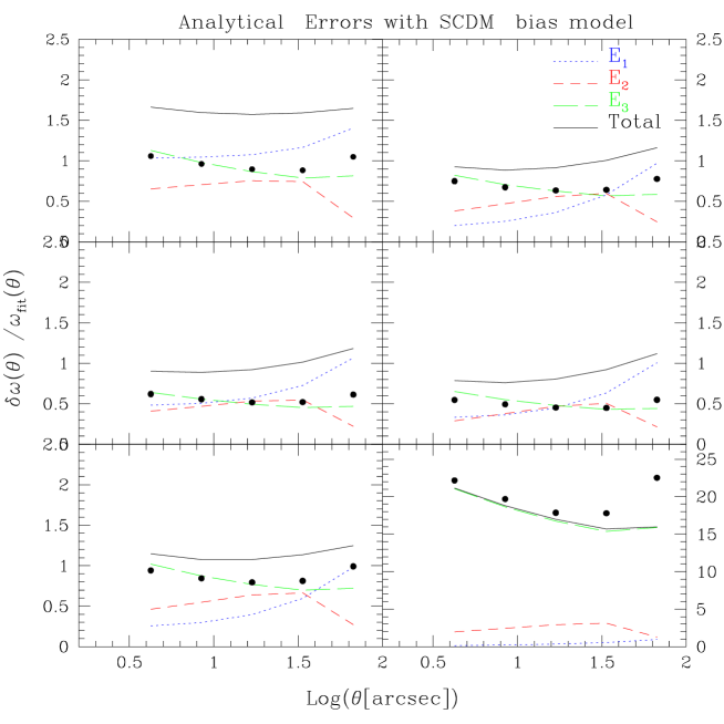
Figure 8: Comparison between the nearly Poissonian errorbars [equation (3), filled circles] used in the computation of $\omega(\theta)$ (Classical ACF) at different angular separations with the analytical errors of equation (LABEL:ece): finite volume error $E_{1}^{1/2}$ (dotted line); discreteness errors $E_{2}^{1/2}$ (short-dashed line), $E_{3}^{1/2}$ (long-dashed line) and total cosmic error $E^{1/2}\equiv(E_{1}+E_{2}+E_{3})^{1/2}$ (solid line). The analytical errors are computed using the $SCDM$ bias model (see § 4.2 for details). The different panels correspond to the different redshift ranges as in Figure 5.

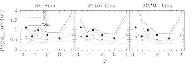
Figure 9: Comparison of the nearly Poissonian errorbars (equation (3) at 10 arcsec, estimated for the HDF-South (filled circles) and the HDF-North (open squares) with the cosmic errors from equation (LABEL:ece) (total: solid lines; $E_{1}$: dotted lines; $E_{2}$: short-dashed lines; $E_{3}$: long-dashed lines). The left, middle and right panels refer to the no bias, the $SCDM$ bias and the $\Lambda CDM$ bias models, respectively (see text). There is one filled circle missing on each panel at $z=4$, which corresponds to a very large Poisson errorbar $\delta\omega/\omega_{\rm fit}\sim 23$ (see the right bottom panel of Figure 8).

In order to quantify how the Advanced Camera on the HST (Pirzkal et al. 2001) can improve the clustering measurements of HDF-like populations, we have estimated the analytical behaviour of the cosmic errors with redshift. The results are shown for $\theta=10^{\prime\prime}$ in Figure 10, which can be directly compared with Figure 9. To estimate the cosmic errors in Figure 10, we have rescaled the mean observed number of galaxies in the HDF-South and North to the respective area of the Advanced Camera (i.e. by a factor $5.33$) and recomputed the term $\overline{\omega}_{\theta_{\rm max}}$ according to the new area, assuming a square geometry. Other quantities, in particular $b(z)$ and the amplitude $\omega(10^{\prime\prime})$ are the same as in Figure 9. Note again that the method we use to calculate $\overline{\omega}_{\theta_{\rm max}}$ is likely to overestimate its real value and therefore finite volume effects.

Finite volume errors become smaller due to the larger area covered, while discreteness effects are reduced due to the larger number of objects in the survey. Except at small $z$, where the effect of the bias can make $E_{1}$ dominant again, the sizes of $E_{1}$ and $E_{2}$ are of same order, and $E_{3}$, which contains the pure Poisson noise, is now negligible. Thus, a survey made with the Advanced Camera will no longer be dominated by shot-noise. In terms of sampling strategy, we find that this kind of survey will be a good compromise between finite volume effects and discreteness effects (e.g. Colombi, Szapudi & Szalay 1998), with a gain of more than a factor two for the total cosmic errors compared to the present data, at least at the scale considered here.

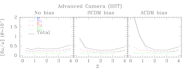
Figure 10: As Figure 9, but in the case of a survey with the Advanced Camera (see text). Only the theoretical cosmic errors from equation (LABEL:ece) are displayed.

5 Conclusions

In this paper, we have described the measurement of the galaxy clustering as a function of $z$ in the HDF-South based on a combination of optical HST data and VLT/ISAAC infrared data. The main results can be summarized as follows:

• The redshift distribution obtained for the HDF-South up to $I_{AB}\sim 27.5$ is consistent with that observed for the HDF-North. The peak of $N(z)$ is close to $z\sim 0.8$ with a decrease at $z\simeq 1$, a plateau from $1\leq z\leq 3$, followed by a decline of the number of objects up to $z\simeq 4.5$.

• We have described an alternative approach to include photometric redshift uncertainties in the ACF measurements. The method is based on a weighted measurement of the ACF taking into account the redshift probability distribution of each object. This method makes it possible to extract the clustering signal with higher significance. It will be interesting to implement and to test the method also for ground-based data which typically have larger photometric errors than HST data, and for less reliable photometric redshift, i.e. with a larger spread of the redshift probability distribution. This approach can be extended to any kind of evolutionary studies based on photometric redshifts, like, for example, the luminosity function.

• We have compared the results of the clustering evolution obtained in the HDF-North and HDF-South. Both are fully consistent within the Poissonian uncertainties. The new observations confirm our previous findings for the HDF-North (A99). The clustering amplitude shows a decrease between $0\leq z\leq 1$ and an increase at $z\geq 1.5$. The redshift range $1\leq z\leq 2$ seems to be a critical epoch where the HDF-galaxy clustering reaches a constant regime still difficult to characterize, due to the smallness of the present sample and to the critical redshift range for photometric redshift determination. Larger samples with the HST Advanced Camera will improve significantly the present picture. The comparison with the behaviour of the underlying dark matter shows that the HDF-galaxy population is a nearly unbiased or anti-biased tracer of the dark matter distribution at $z\leq 1$ and $z\leq 1.5$ in $SCDM$ and $\Lambda CDM$ models, respectively. At higher redshift the clustering amplitude increases and the bias of this population too. At $\langle z\rangle\simeq 3$, the bias is $b\simeq 3$ and $b\simeq 2$ for $SCDM$ and $\Lambda CDM$ models, respectively. This is in good agreement with the results we obtained for HDF-North (see also Magliocchetti & Maddox 1999). The typical minimum masses of the hosting dark matter haloes required to reproduce the observations in $SCDM$ model are $M_{\rm min}=10^{10}h^{-1}M_{\odot}$ at $z\leq 1.5$ and $M_{\rm min}\simeq 10^{11}h^{-1}M_{\odot}$ for $1.5\leq z\leq 3.5$ ($M_{\rm min}\leq 10^{10}h^{-1}M_{\odot}$ at $z\leq 1.5$ and $M_{\rm min}\simeq 10^{11-11.5}h^{-1}M_{\odot}$ for $1.5\leq z\leq 3.5$ in $\Lambda CDM$ model). At $\langle z\rangle\simeq 4$, the clustering signal detected in the HDF-South is considerably smaller than the corresponding amplitude observed in the northern field, but, due to the very small sample (and, as a consequence, a large Poisson noise), the two results are still consistent within $1\sigma$. Again, larger samples are required at such a redshift.

• In all our analysis we used errorbars assuming nearly Poisson statistics ($w(\theta)\ll 1$), as given by Landy & Szalay (1993). To check a posteriori that such a procedure is valid, we used the analytical approach of Bernstein (1994), which fully describes the global budget of cosmic errors. In particular, the formulae obtained by Bernstein (1994) do not assume $\omega(\theta)\ll 1$ and take into account effects of higher-order statistics. We checked that we recover the nearly-Poissonian contribution in Bernstein’s calculations, and we found that it is indeed dominant in most regimes, except at small redshifts and at large angular scales, where the finite volume error (often called cosmic variance) can become significant. Note that Bernstein’s calculations neglect the edge effects, which can contribute to the errors (e.g. Szapudi & Colombi 1996). However, by construction, the Landy & Szalay estimator, that we used in our analysis, should minimize them to a large extent.

  As a general conclusion of this paper, the HDF samples allowed us to obtain a global picture of the redshift evolution of the galaxy clustering, but with errorbars dominated by Poisson noise. Future instruments, like the Advanced Camera, will improve the accuracy of the measurement of $\omega(\theta)$ by at least a factor two, mainly by reducing discreteness errors. In particular, pure Poisson noise will become subdominant and it will no longer be possible to neglect finite volume effects in the analyses.

References

- [ASGDPK98] Adelberger K.L., Steidel C.C., Giavalisco M., Dickinson M.E., Pettini M., Kellogg M., 1998, ApJ, 505, 18
- [A99] Arnouts S., Cristiani S., Moscardini L., Matarrese S., Lucchin F., Fontana A., Giallongo E., 1999, MNRAS, 310, 540 (A99)
- [Benitez00] Benítez, N., 2000, ApJ, 536, 571
- [] Benoist C., Maurogordato S., da Costa L.N., Cappi A., Schaeffer R., 1996, ApJ, 472, 452
- [1] Bernardeau F., 1994, A&A, 291, 697
- [2] Bernardeau F., Schaeffer R., 1992, A&A, 255, 1
- [3] Bernardeau F., Schaeffer R., 1999, A&A, 349, 697
- [] Bernstein G.M., 1994, ApJ, 424, 569
- [] Bertin E., Arnouts S., 1996, A&AS, 117, 393
- [] Bolzonella M., Miralles J.-M., Pellò R., 2000, A&A, 363, 476
- [] Bruzual G., Charlot S., 1993, ApJ, 405, 538
- [] Carlberg R.G., Cowie L.L., Songaila A., Hu E.M., 1997, ApJ, 484, 538
- [] Carlberg R.G., Yee H.K.C., Morris S.L., Lin H., Hall P.B., Patton D., Sawicki M., Shepherd C.W., 2000, ApJ, 542, 57
- [] Casertano S. et al., 2000, AJ, 120, 2747
- [] Catelan P., Lucchin F., Matarrese S., Porciani C., 1998, MNRAS, 297, 692
- [] Cohen J. G., Hogg D., Blandford R., Cowie L., Hu E., Songaila A., Shopbell P., Richberg K., 2000, ApJ, 538, 29
- [] Colombi S., Bouchet F.R., Hernquist L., 1996, ApJ, 465, 14
- [] Colombi S., Charlot S., Devriendt J.E.G., Fioc M., Szapudi I., 2000, in Clustering at High Redshift, eds. A. Mazure, O. Le Fèvre & V. Le Brun, ASP Conference Series 200, p. 153
- [] Colombi S., Szapudi I., Szalay A.S., 1998, MNRAS, 296, 253
- [] Connolly A.J., Szalay A.S., Brunner R.J., 1998, ApJ, 499, L125
- [] Cristiani S. et al., 2000, A&A, 359, 489-492
- [] Dennefeld et al., 2001, in preparation
- [] Eke V. R., Cole S., Frenk C. S., 1996, MNRAS, 282, 263
- [] Fernández-Soto A., Lanzetta K. M., Yahil A., 1999, ApJ, 513, 34
- [] Gaztañaga E., 1994, MNRAS, 268, 913
- [] Giavalisco M., Dickinson M., 2001, ApJ, 550, 177
- [] Giavalisco M., Steidel C.C., Adelberger K.L., Dickinson M.E., Pettini M., Kellogg M., 1998, ApJ, 503, 543
- [] Glazebrook et al., 1998, in preparation (http://www.aao.gov.au/hdfs/Redshifts/)
- [] Hamilton A.J.S, 1993, ApJ, 417, 19
- [] Hamilton A.J.S., Kumar P., Lu E., Mathews A., 1991, ApJ, 374, L1
- [] Hogg D.W., Cohen J.C., Blandford R., 2000, ApJ, 545, 32
- [] Jain B., Mo H.J., White S.D.M., 1995, MNRAS, 276, L25
- [] Jenkins A. et al., 1998, ApJ, 499, 20
- [] Jing Y.P., 1999, ApJ, 515, L45
- [] Juszkiewicz R., Bouchet F.R., Colombi S., 1993, ApJ, 412, L9
- [] Kaiser N., 1984, ApJ, 284, L9
- [] Landy S.D., Szalay A.S., 1993, ApJ, 412, 64 (LS93)
- [] Lanzetta K.M., Yahil A., Fernández-Soto A., 1996, Nat, 381, 759
- [] Le Fèvre O., Hudon D., Lilly S.J., Crampton D., Hammer F., Tresse L., 1996, ApJ, 461, 534
- [] Loveday J., Maddox S.J., Efstathiou G., Peterson B.A., 1995, ApJ, 442, 457
- [] Maddox S.J., Efstathiou G., Sutherland W.J., Loveday J., 1990, MNRAS, 242, 43P
- [] Magliocchetti M., Maddox S.J., 1999, MNRAS, 306, 988
- [] Matarrese S., Coles P., Lucchin F., Moscardini L., 1997, MNRAS, 286, 115
- [] Mo H.J., White S.D.M., 1996, MNRAS, 282, 347
- [] Moscardini L., Coles P., Lucchin F., Matarrese S., 1998, MNRAS, 299, 95
- [] Moscardini L., Matarrese S., De Grandi S., Lucchin F., 2000a, MNRAS, 314, 647
- [] Moscardini L., Matarrese S., Lucchin F., Rosati P., 2000b, MNRAS, 316, 283
- [] Norberg P., Baugh C.M., Hawkins E., Maddox S. , Peacock J.A. et al., 2001, astro-ph/0105500
- [] Peacock J.A., Dodds S.J., 1994, MNRAS, 267, 1020
- [] Peacock J.A., Dodds S.J., 1996, MNRAS, 280, L19
- [] Peebles P.J.E., 1974, A&A, 32, 391
- [] Pirzkal N., Pasquali A., Hook R., Walsh J., Fosbury R., Freudling W., Albrecht R., 2001, to appear in the proceedings of the “Deep Fields” conference, in press
- [] Roukema B.F., Valls-Gabaud D., Mobasher B., Bajtlik S., 1999, MNRAS, 305, 105
- [] Santiago B.X., da Costa L.N., 1990, ApJ, 362, 386
- [] Saracco P., Giallongo E., Cristiani S., d’Odorico S., Fontana A., Iovino A., Poli F., Vanzella E., 2001, A&A, in press, astro-ph/0104284
- [] Sawicki M.J., Lin H., Yee H.K.C., 1997, AJ, 113, 1
- [] Sheth R.K., Mo H.J., Tormen G., 2001, MNRAS, 323, 1
- [] Sheth R.K., Tormen G., 1999, MNRAS, 308, 119
- [] Small T.A., Ma C.-P., Sargent W.L.W., Hamilton D., 1999, ApJ, 524, 31
- [] Steidel C.C., Giavalisco M., Pettini M., Dickinson M., Adelberger K.L., 1996, ApJ, 462, L17
- [] Szapudi I., 2000, to appear in the proceedings of the 15th Florida Workshop in Nonlinear Astronomy and Physics, The Onset of Nonlinearity, astro-ph/0008224
- [] Szapudi I., Colombi S., 1996, ApJ, 470, 131
- [] Szapudi I., Postman M., Lauer T., Oegerle W., 2001, ApJ, 548, 114
- [] Szapudi I., Quinn T., Stadel J., Lake G., 1999, ApJ, 517, 54
- [] Vanzella E., Cristiani S., Saracco P., Arnouts S., Bianchi S., d’Odorico S., Fontana A., Giallongo E., Grazian A., 2001, to appear in AJ (astro-ph/0107506)
- [] Williams R.E. et al., 1996, AJ, 112, 1335