Inflationary Cosmology: Theory and Phenomenology

Abstract

This article gives a brief overview of some of the theory behind the inflationary cosmology, and discusses prospects for constraining inflation using observations. Particular care is given to the question of falsifiability of inflation or of subsets of inflationary models.

1 Overview

This being the first talk/article of the conference, I begin with a brief reminder of what we are currently trying to achieve in cosmology. Personally, I’m interested in the following overall goals:

• To obtain a physical description of the Universe, including its global dynamics and matter content.

• To measure the cosmological parameters describing the Universe, and to develop a fundamental understanding of as many of those parameters as possible.

• To understand the origin and evolution of cosmic structures.

• To understand the physical processes which took place during the extreme heat and density of the early Universe.

Over recent years, much progress has been made on all of these topics, to the extent that it is widely believed amongst cosmologists that we may stand on the threshold of the first precision cosmology, in which the parameters necessary to describe our Universe have been identified and, in most cases at least, measured to a satisfying degree of precision. Whether this optimism has any grounding in reality remains to be seen, though so far the signs are promising in that the basic picture of cosmology, centred around the Hot Big Bang, has time and again proven the best framework for interpretting the constantly improving observational situation.

In particular, the process of cosmological parameter estimation is well underway, thanks to observations of distant Type Ia supernovae, of galaxy clustering, and of the cosmic microwave background. These have established a standard cosmological model, where the Universe is dominated by dark energy, contains substantial dark matter, and with the baryons from which we are made comprising only around 5%. Overall this model can be described by around ten parameters (e.g. see Wang et al. [1]), and the viable region of parameter space is starting to shrink under pressure from observations. However, it is worth bearing in mind that we seek high precision determinations at least in part because they ought to shed light on fundamental physics, and there progress has been less rapid. Some parameters are likely to have no particular fundamental importance (for instance, there would probably be little fundamental significance were the Hubble constant to turn out to be $63\,{\rm km\,s}^{-1}\,{\rm Mpc}^{-1}$ rather than say $72\,{\rm km\,s}^{-1}\,{\rm Mpc}^{-1}$), but the 10% or so measured accuracy of the baryon density is to be set against the lack of even an order-of-magnitude theoretical understanding thus far.

2 Inflationary cosmology: models

This article focusses on the last two of the goals listed at the start of the previous section. The claim is that during the very early Universe, a physical process known as inflation took place, which still manifests itself in our present Universe via the perturbations it left behind which later led to the development of structure in the Universe. By studying those structures, we hope to shed light on whether inflation occurred, and by what physical mechanism.

I begin by defining inflation. The scale factor of the Universe at a given time is measured by the scale factor $a(t)$. In general a homogeneous and isotropic Universe has two characteristic length scales, the curvature scale and the Hubble length. The Hubble length is more important, and is given by

$$cH^{-1}\quad{\rm where}\quad H\equiv\frac{\dot{a}}{a}\,.$$ (1)

Typically, the important thing is how the Hubble length is changing with time as compared to the expansion of the Universe, i.e. what is the behaviour of the comoving Hubble length $H^{-1}/a$?

During any standard evolution of the Universe, such as matter or radiation domination, the comoving Hubble length increases. It is then a good estimate of the size of the observable Universe. Inflation is defined as any epoch of the Universe’s evolution during which the comoving Hubble length is decreasing

$$\frac{d\left(H^{-1}/a\right)}{dt}<0\Longleftrightarrow\ddot{a}>0\,,$$ (2)

and so inflation corresponds to any epoch during which the Universe has accelerated expansion. During this time, the expansion of the Universe outpaces the growth of the Hubble radius, so that physical conditions can become correlated on scales much larger than the Hubble radius, as required to solve the horizon and flatness problems.

As it happens, there is very good evidence from observations of Type Ia supernovae that the Universe is presently accelerating — see the article by Schmidt in these proceedings and Ref. [2]. This is usually attributed to the presence of a cosmological constant. This is clearly at some level good news for those interested in the possibility of inflation in the early Universe, as it indicates that inflation is possible in principle, and certainly that any purely theoretical arguments which suggest inflation is not possible should be treated with some skepticism.

If the Universe contains a fluid, or combination of fluids, with energy density $\rho$ and pressure $p$, then

$$\ddot{a}>0\Longleftrightarrow\rho+3p<0\,,$$ (3)

(where the speed of light $c$ has been set to one). As we always assume a positive energy density, inflation can only take place if the Universe is dominated by a material which can have a negative pressure. Such a material is a scalar field, usually denoted $\phi$. A homogeneous scalar field has a kinetic energy and a potential energy $V(\phi)$, and has an effective energy density and pressure given by

$$\rho=\frac{1}{2}\dot{\phi}^{2}+V(\phi)\quad;\quad p=\frac{1}{2}\dot{\phi}^{2}-V(\phi)\,.$$ (4)

The condition for inflation can be satisfied if the potential dominates.

A model of inflation typically amounts to choosing a form for the potential, perhaps supplemented with a mechanism for bringing inflation to an end, and perhaps may involve more than one scalar field. In an ideal world the potential would be predicted from fundamental particle physics, but unfortunately there are many proposals for possible forms. Instead, it has become customary to assume that the potential can be freely chosen, and to seek to constrain it with observations. A suitable potential needs a flat region where the potential can dominate the kinetic energy, and there should be a minimum with zero potential energy in which inflation can end. Simple examples include $V=m^{2}\phi^{2}/2$ and $V=\lambda\phi^{4}$, corresponding to a massive field and to a self-interacting field respectively. Modern model building can get quite complicated — see Ref. [3] for a review.

3 Inflationary cosmology: perturbations

By far the most important aspect of inflation is that it provides a possible explanation for the origin of cosmic structures. The mechanism is fundamentally quantum mechanical; although inflation is doing its best to make the Universe homogeneous, it cannot defeat the uncertainty principle which ensures that residual inhomogeneities are left over. These are stretched to astrophysical scales by the inflationary expansion. Further, because these are determined by fundamental physics, their magnitude can be predicted independently of the initial state of the Universe before inflation. However, the magnitude does depend on the model of inflation; different potentials predict different cosmic structures.

One way to think of this is that the field experiences a quantum ‘jitter’ as it rolls down the potential. The observed temperature fluctuations in the cosmic microwave background are one part in $10^{5}$, which ultimately means that the quantum effects should be suppressed compared to the classical evolution by this amount.

Inflation models generically predict two independent types of perturbation:

Density perturbations $\delta_{{\rm H}}^{2}(k)$:

These are caused by perturbations in the scalar field driving inflation, and the corresponding perturbations in the space-time metric.

Gravitational waves $A_{{\rm T}}^{2}(k)$:

These are caused by perturbations in the space-time metric alone.

They are sometimes known as scalar and tensor perturbations respectively, because of the way they transform. Density perturbations are responsible for structure formation, but gravitational waves can also affect the microwave background.

We do not expect to be able to predict the precise locations of cosmic structures from first principles (any more than one can predict the precise position of a quantum mechanical particle in a box). Rather, we need to focus on statistical measures of clustering. Simple models of inflation predict that the amplitudes of waves of a given wavenumber $k$ obey gaussian statistics, with the amplitude of each wave chosen independently and randomly from a gaussian. What it does predict is how the width of the gaussian, known as its amplitude, varies with scale; this is known as the power spectrum.

With current observations it is a good approximation to take the power spectra as being power laws with scale, so

$$\delta_{{\rm H}}^{2}(k) = \delta_{{\rm H}}^{2}(k_{0})\left[\frac{k}{k_{0}}\right]^{n-1}$$ (5)

$$A_{{\rm T}}^{2}(k) = A_{{\rm T}}^{2}(k_{0})\left[\frac{k}{k_{0}}\right]^{n_{{\rm T}}}$$ (6)

In principle this gives four parameters — two amplitudes and two spectral indices — but in practice the spectral index of the gravitational waves is unlikely to be measured with useful accuracy, which is rather disappointing as the simplest inflation models predict a so-called consistency relation relating $n_{{T}}$ to the amplitudes of the two spectra, which would be a distinctive test of inflation. The assumption of power-laws for the spectra requires assessment both in extreme areas of parameter space and whenever observations significantly improve.

4 Testing inflation

4.1 Quantifying microwave background anisotropies

Although the strongest tests of cosmological models will always come from the combination of all available data, for the particular purpose of constraining inflation it is likely that the cosmic microwave background anisotropies will be the single most useful type of observation, and so it is worth spending some time defining the relevant terminology.

We observe the temperature $T(\theta,\phi)$ coming from different directions. We write this as a dimensionless perturbation and expand in spherical harmonics

$$\frac{T(\theta,\phi)-\bar{T}}{\bar{T}}=\sum_{\ell,m}a_{\ell m}\,Y^{\ell}_{m}(\theta,\phi)\,.$$ (7)

Again there is no unique prediction for the coefficients $a_{\ell m}$, but they are drawn from a gaussian distribution whose mean square is independent of $m$ and given by the radiation angular power spectrum

$$C_{\ell}=\left\langle\left|a_{\ell m}\right|^{2}\right\rangle_{{\rm ensemble}}$$ (8)

The ensemble average represents the theorist’s ability to average over all possible observers in the Universe (or indeed over different quantum mechanical realizations), whereas an observer’s highest ambition is to estimate it by averaging over the multipoles of different $m$ as seen at our own location. The radiation angular power spectrum depends on all the cosmological parameters, and so it can be used to constrain them. To extract the full information, polarization also has to be measured.

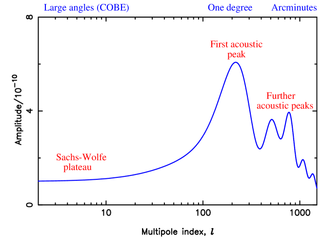
Figure 1: The radiation angular power spectrum for a particular cosmological model. The annotations name the different features, as discussed later in this article.

Computation of the power spectrum requires a lot of physics: gravitational collapse, photon–electron interactions (and their polarization dependence), neutrino free-streaming etc. But as long as the perturbations are small, linear perturbation theory can be used which makes the calculations possible. A major step forward for the field was the public release of Seljak & Zaldarriaga’s code cmbfast [5] which can compute the spectrum for a given cosmological model in around one minute. An example spectrum is shown in Figure 1.

4.2 The key tests of inflation

In the remainder of this article, I will be interested solely in inflation as a model for the origin of structure; while it serves a useful purpose in solving the horizon and flatness problems these are no longer likely to provide further tests of the model. Indeed, the aim is to consider inflation as the sole origin of structure, since it is impossible to exclude an admixture of inflationary perturbations at some level even if another mechanism becomes favoured.

The key tests of inflation can be summarized in one very useful sentence, which lists in bold-face six key predictions that we would like to test.

The simplest models of inflation predict nearly power-law spectra of adiabatic, gaussian scalar and tensor perturbations in their growing mode in a spatially-flat Universe.

However some tests are more powerful than others, because some are predictions only of the simplest inflationary models. In what follows, it will be important to distinguish between tests of the inflationary idea itself, versus tests of different inflationary models or classes of models.

Before progressing to a discussion of the status of these tests, it is useful to define some terminology fairly precisely. In this article, a useful test of a model is one which, if failed, leads to rejection of that model. The concept of a test is to be contrasted with supporting evidence, which is verification of a prediction which, while not generic, is seen as indicative that the model is correct. A model can also accrue supporting evidence via its rivals failing to survive tests that they are put to.

4.2.1 Spatial flatness

All the standard models of inflation give a flat Universe, and this used to be advertised as a robust prediction. Unfortunately we now realise that it is possible to make more complicated models which can give an open Universe [6]. Spatial geometry therefore does not constitute a test of the inflationary paradigm, as if the Universe were not flat there would remain viable inflationary models. However the recent microwave anisotropy experiments showing good consistency with spatial flatness (see the article by Lasenby in these proceedings) provide good supporting evidence for the simplest inflation models.

4.2.2 Gaussianity and adiabaticity

If inflation is driven by more than one scalar field, there is a possibility of having isocurvature perturbations as well as adiabatic ones. The mechanism is that during inflation the other fields also receive perturbations. If they survive to the present (in particular, if they become the dark matter), this will give an isocurvature perturbation. As far as model building is concerned, such isocurvature perturbations could dominate, though this is now excluded by observations. More pertinently, the observed structures could be due to an admixture of adiabatic and isocurvature perturbations, and indeed those modes could be correlated.

Such models would also give either gaussian or nongaussian perturbations, and nongaussian adiabatic models are also possible. Whether observed nongaussianity rules out inflation depends very much on the type of nongaussianity observed; for instance chi-squared distributed fluctuations could easily be produced if the leading contribution to the perturbations is quadratic in the scalar field perturbation, while if any coherent spatial structures were seen, such as line discontinuities in the microwave background, it would be futile to try and produce them using inflation.

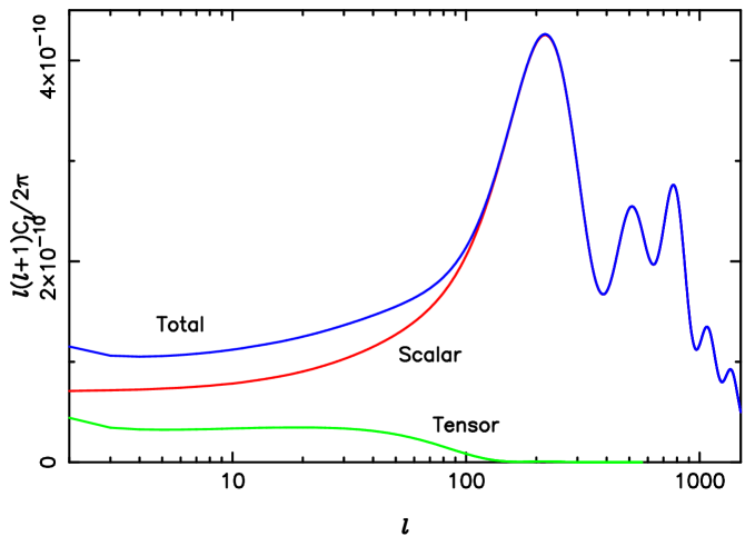
Figure 2: Scalars and tensors give different contributions to the anisotropies. While only the total spectrum is observable, provided the spectra have sufficiently simple forms this can be decomposed into the two parts, the tensors giving excess perturbations at small $\ell$.

4.2.3 Vector and tensor perturbations

All inflation models produce gravitational waves at some level, and if seen they can provide extremely strong supporting evidence for inflation. They are not however a test, as their absence could mean an inflation model where their amplitude is undetectably small. The best way to detect them is by their contribution to large-angle anisotropies, as shown in Figure 2.

By contrast, known inflation models do not produce vector perturbations, and indeed inflation will destroy any pre-existing ones. If detected, at the very least they would present a challenge for inflation model builders. It would be interesting to make a comprehensive study to confirm whether detection of vector modes would be sufficient to exclude inflation as the sole origin of structure.

4.2.4 Growing mode perturbations

A key property of inflationary perturbations is that they were created in the early Universe and evolved freely from then. Although a general solution to the perturbation equations has two modes, growing and decaying, only the growing mode will remain by the time the perturbation enters the horizon. This leads directly to the prediction of an oscillatory structure in the microwave anisotropy power spectrum, as seen in Figure 1 [7]. The existence of such a structure is a robust prediction of inflation; if it is not seen then inflation cannot be the sole origin of structure.

The most significant recent development in observations pertaining to inflation is the first clear evidence for multiple peaks in the spectrum, seen by the DASI [8] and Boomerang [9] experiments. This is a crucial qualitative test which inflation appears to have passed, and which could have instead provided evidence against the entire inflationary paradigm. These observations lend great support to inflation, though it must be stressed that they are not able to ‘prove’ inflation, as it may be that there are other ways to produce such an oscillatory structure [10].

5 Present and future

5.1 The current status of inflation

The best available constraints come from combining data from different sources; for two recent attempts see Wang et al. [1] and Efstathiou et al. [11]. Suitable data include observations of the recent dynamics of the Universe using Type Ia supernovae, cosmic microwave anisotropy data, and galaxy correlation function data such as that described by Lahav and by Frieman in these proceedings.

Currently inflation is a massive qualitative success, with striking agreement between the predictions of the simplest inflation models and observations. In particular, the locations of the microwave anisotropy power spectrum peaks are most simply interpretted as being due to an adiabatic initial perturbation spectrum in a spatially-flat Universe. The multiple peak structure strongly suggests that the perturbations already existed at a time when their corresponding scale was well outside the Hubble radius. No unambiguous evidence of nongaussianity has been seen.

Quantitatively, however, things have some way to go. At present the best that has been done is to try and constrain the parameters of the power-law approximation to the inflationary spectra. The gravitational waves have not been detected and so their amplitude has only an upper limit and their spectral index is not constrained at all. The current situation can be summarized as follows.

Amplitude $\delta_{{\rm H}}$:

COBE determines this (assuming no gravitational waves) to about ten percent accuracy (at one-sigma) as approximately $\delta_{{\rm H}}=1.9\times 10^{-5}\,\Omega_{0}^{-0.8}$ on a scale close to the present Hubble radius (see Refs. [12, 4] for accurate formulae).

Spectral index $n$:

This is thought to lie in the range $0.8<n<1.05$ (at 95% confidence). It would be extremely interesting were the scale-invariant case, $n=1$, to be convincingly excluded, as that would be clear evidence of dynamical processes at work, rather than symmetries, in creating the perturbations.

Gravitational waves $r$:

Measured in terms of the relative contribution to large-angle microwave anisotropies, the tensors are currently constrained to be no more than about 30%.

5.2 Prospects for the future

It remains possible that future observations will slap us in the face and lead to inflation being thrown out. But if not, we can expect an incremental succession of better and better observations, culminating (in terms of currently-funded projects) with the Planck satellite [13]. Faced with observational data of exquisite quality, an initial goal will be to test whether the simplest models of inflation continue to fit the data, meaning models with a single scalar field rolling slowly in a potential $V(\phi)$ which is then to be constrained by observations. If this class of models does remain viable, we can move on to reconstruction of the inflaton potential from the data.

Planck, currently scheduled for launch in February 2007, should be highly accurate. In particular, it should be able to measure the spectral index to an accuracy better than $\pm 0.01$, and detect gravitational waves even if they are as little as 10% of the anisotropy signal. In combination with other observations, these limits could be expected to tighten significantly further, especially the tensor amplitude. Such observations would rule out almost all currently known inflationary models. Even so, there will be considerable uncertainties, so it is important not to overstate what can be achieved.

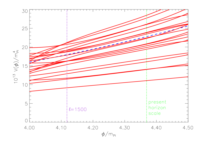
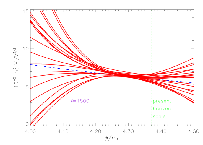
Figure 3: Sample reconstruction of a potential, where the dashed line shows the true potential and the solid lines are thirty Monte Carlo reconstructions (real life can only provide one). The upper panel shows the potential itself which is poorly determined. However some combinations, such as $(dV/d\phi)/V^{3/2}$ shown in the lower panel, can be determined at an accuracy of a few percent. See Ref. [14] for details.

Reconstruction can only probe the small part of the potential where the field rolled while generating perturbations on observable scales. We know enough about the configuration of the Planck satellite to be able to estimate how well it should perform. Ian Grivell and I recently described a numerical technique which gives an optimal construction [14]. Results of an example reconstruction are shown in Figure 3, where it was assumed that the true potential was $\lambda\phi^{4}$. The potential itself is not well determined here (the tensors are only marginally detectable), but certain combinations, such as $(dV/d\phi)/V^{3/2}$, are accurately constrained and would lead to high-precision constraints on inflation model parameters.

6 New directions

While the simplest models of inflation provide an appealing simple framework giving excellent agreement with observations, it is important to consider whether a similar outcome might arise from a more complicated set-up that has better motivation from fundamental physics. There are some new ideas circulating in this regard, of which I will highlight just two related ones.

6.1 The braneworld

Particle physicists generally tend to believe that our Universe really possesses more than three spatial dimensions. Previously it has been assumed that the extra ones were “curled up” to be unobservably small. A new idea is the braneworld, which proposes that at least one of these extra dimensions might be relatively large, with us constrained to live on a three-dimensional brane running through the higher-dimensional space. Gravity is able to propagate in the full higher-dimensional space, which is known as the bulk.

This radical idea has many implication for cosmology, both in the present and early Universe, and so far we have only scratched the surface of possible new phenomena. Already many exciting results have been obtained – see the article by Wands in these proceedings. I’ll just consider a few pertinent questions.

1. Are there modifications to the evolution of the homogeneous Universe?
The answer appears to be yes; for example in a simple scenario (known as Randall–Sundrum Type II [15]) the Friedmann equation is modified at high energies so that, after some simplifying assumptions, it reads [16]

$$H^{2}=\frac{8\pi G}{3}\left(\rho+\frac{\rho^{2}}{2\lambda}\right)\,,$$ (9)

where $\lambda$ is the tension of the brane. This recovers the usual cosmology at low energies $\rho\ll\lambda$, but otherwise we have new behaviour. This opens new opportunities for model building, see for example Ref. [17].

2. Are inflationary perturbations different?
Again the answer is yes — there are modifications to the formulae giving scalar and tensor perturbations [18]. Unfortunately the main effect of this is to introduce new degeneracies in interpretting observations, as a potential can always be found matching observations for any value of $\lambda$ [19]. The initial perturbations therefore cannot be used to test the braneworld scenario.

3. Do perturbations evolve differently after they are laid down on large scales?
The answer here is less clear. It is certainly possible that perturbation evolution is modified even at late times. For example perturbations in the bulk could influence the brane in a way that couldn’t be predicted from brane variables alone. Whether there is a significant effect is unclear and is likely to be model dependent.

6.2 The Ekpyrotic Universe

It has recently been proposed that the Big Bang is actually the result of the collision of two branes, dubbed the Ekpyrotic Universe [20]; this scenario is discussed in detail in Turok’s article in these proceedings. It has been claimed that this scenario can provide a resolution to the horizon and flatness problems, essentially because causality arises from the higher-dimensional theory and allows a simultaneous Big Bang everywhere on our brane, though existing implementations solve the problem by hand in the initial conditions. As I write this, it remains unclear how to successfully describe the instant of collision between the two branes (the singularity problem), and considerable controversy surrounds whether or not the scenario can also generate nearly scale-invariant adiabatic perturbations [21]. Both aspects are required to make it a serious rival to inflation.

7 Summary

These are extremely good times for the inflationary cosmology. Its qualitative predictions have time and again provided the simplest interpretation of observational data, while historical rivals such as cosmic strings [22] have faded away. There is every prospect that upcoming observations will provide high-accuracy constraints on the models devised. The necessary theoretical ingredients all appear to be in place to allow predictions of the required sophistication to be made. We keenly await new observational data.

References

References

- [1] X. Wang, M. Tegmark and M. Zaldarriaga, astro-ph/0105091.
- [2] S. Perlmutter, Nature 391, 51 (1998); A. G. Riess et al., Astronomical. J. 116, 1009 (1998); S. Perlmutter et al., Astrophys. J. 517, 565 (1999).
- [3] D. H. Lyth and A. Riotto, Phys. Rep. 314, 1 (1999).
- [4] A. R. Liddle and D. H. Lyth, Cosmological inflation and large-scale structure, Cambridge University Press (2000).
- [5] U. Seljak and M. Zaldarriaga, Astrophys. J. 469, 1 (1996).
- [6] J. R. Gott, Nature 295, 304 (1982); M. Sasaki, T. Tanaka, K. Yamamoto and J. Yokoyama, Phys. Lett. B 317, 510 (1993); M. Bucher, A. S. Goldhaber and N. Turok, Phys. Rev. D 52, 3314 (1995).
- [7] A. Albrecht, D. Coulson, P. Ferreira and J. Magueijo, Phys. Rev. Lett. 76, 1413 (1996); A. Albrecht in Critical Dialogues in Cosmology, ed N. Turok, World Scientific 1997, astro-ph/9612017; W. Hu and M. White, Phys. Rev. Lett. 77, 1687 (1996).
- [8] N. W. Halverson et al., astro-ph/0104489; C. Pryke et al., astro-ph/0104490.
- [9] C. B. Netterfield et al., astro-ph/0104460; P. de Bernardis et al., astro-ph/0105296.
- [10] N. Turok, Phys. Rev. Lett. 77, 4138 (1996).
- [11] G. Efstathiou et al., astro-ph/0109152.
- [12] E. F. Bunn and M. White, Astrophys. J. 480, 6 (1997); E. F. Bunn, A. R. Liddle and M. White, Phys. Rev. D 54, 5917R (1996).
-
[13]
Planck home page at
http://astro.estec.esa.nl/Planck/ - [14] I. J. Grivell and A. R. Liddle, Phys. Rev. D 61, 081301 (2000).
- [15] L. Randall and R. Sundrum, Phys. Rev. Lett. 83, 4690 (1999).
- [16] P. Binétruy, C. Deffayet and D. Langlois, Nucl. Phys. B565 (2000) 269; P. Binétruy, C. Deffayet, U. Ellwanger and D. Langlois, Phys. Lett. B477, 285 (2000); T. Shiromizu, K. Maeda and M. Sasaki, Phys. Rev. D62, 024012 (2000).
- [17] E. J. Copeland, A. R. Liddle and J. E. Lidsey, Phys. Rev. D 64, 023509 (2001).
- [18] R. Maartens, D. Wands, B. A. Bassett, and I. P. C. Heard, Phys. Rev. D62, 041301 (2000); D. Langlois, R. Maartens, and D. Wands, Phys. Lett B489, 259 (2000).
- [19] A. R. Liddle and A. N. Taylor, astro-ph/0109412.
- [20] J. Khoury, B. A. Ovrut, P. J. Steinhardt and N. Turok, hep-th/0103239 and hep-th/0108187 (see also R. Kallosh, L. Kofman and A. Linde, hep-th/0104073).
- [21] D. H. Lyth, hep-ph/0106153; R. Brandenberger and F. Finelli, hep-th/0109004; J. Khoury, B. A. Ovrut, P. J. Steinhardt and N. Turok, hep-th/0109050; J. Hwang, astro-ph/0109045.
- [22] A. Vilenkin and E. P. S. Shellard, Cosmic strings and other topological defects, Cambridge University Press (1994).