ENERGY BALANCE IN THE SOLAR TRANSITION REGION. IV.
HYDROGEN AND HELIUM MASS FLOWS WITH DIFFUSION

Abstract

In this paper we have extended our previous modeling of energy balance in the chromosphere-corona transition region to cases with particle and mass flows. The cases considered here are quasi-steady, and satisfy the momentum and energy balance equations in the transition region. We include in all equations the flow velocity terms and neglect the partial derivatives with respect to time. We present a complete and physically consistent formulation and method for solving the non-LTE and energy balance equations in these situations, including both particle diffusion and flows of H and He. Our results show quantitatively how mass flows affect the ionization and radiative losses of H and He, thereby affecting the structure and extent of the transition region. Also, our computations show that the H and He line profiles are greatly affected by flows. We find that line shifts are much less important than the changes in line intensity and central reversal due to the effects of flows. In this paper we use fixed conditions at the base of the transition region and in the chromosphere because our intent is to show the physical effects of flows and not to match any particular observations. However, we note that the profiles we compute can explain the range of observed high spectral and spatial resolution Lyman alpha profiles from the quiet Sun. We suggest that dedicated modeling of specific sequences of observations based on physically consistent methods like those presented here will substantially improve our understanding of the energy balance in the chromosphere and corona.

1 Introduction

In our previous papers, Fontenla et al. (1990, 1991, 1993, hereafter FAL1, FAL2, FAL3), we developed quasi-static models of the solar atmosphere, using separate one-dimensional models to represent different quiet and active solar features. These models included a turbulent velocity, both to broaden spectral lines and to add a Bernoulli term in the hydrostatic equilibrium equation to represent a dynamic pressure contribution. The modified equation was used to determine the density stratification in the atmosphere that, because of this added term, departs from a hydrostatic stratification that balances only gas pressure and gravity. We introduced the important effects of hydrogen and helium diffusion in the chromosphere-corona transition region, and for the first time obtained reasonable agreement between calculated and observed line profiles for hydrogen and helium, including general agreement with the well-observed hydrogen Lyman alpha line profile (Fontenla, Reichmann, & Tandberg-Hanssen 1988).

Many papers have studied quasi-steady flows in the transition region, e.g., Boris & Mariska (1982), Craig & McClymont (1986), McClymont & Craig (1987), Mariska (1988), and McClymont (1989). It is not possible for us to address all of them; for a review, see Mariska (1992). Here we just mention that these papers deal in detail with the upper transition region and coronal loops where H and He are fully ionized, and use the radiative losses determined by Cox & Tucker (1969) for optically thin plasmas. These papers do not treat accurately the lower transition region and chromosphere where H and He are only partially ionized and where the resonance lines of H and He must be computed from detailed solutions of the radiative transfer equations. Also, these papers do not include the complicated processes of particle diffusion and radiative transfer addressed by the FAL papers. Despite these shortcomings they indicated that the observed redshifts in transition region lines might be explained by quasi-steady flows in coronal loops.

Other, more recent calculations have been carried out, e.g., by Hansteen & Leer (1995), that include velocities in models assuming a fully ionized plasma. While this assumption is valid in the corona, and perhaps (depending on the velocity) in the upper transition region, it is inadequate for the low transition region where H and He are only partially ionized.

The paper by Woods & Holzer (1991) considers a multicomponent plasma composed of electrons, protons, ionized helium, and minor ion species. These calculations use the St. Maurice & Schunk (1977a, b) treatment of particle diffusion and heat flow (which is based on a different method but in most respects is equivalent to that used in the FAL papers). Woods & Holzer make the point that earlier estimates of minor ion line intensities may not be accurate because the effects of flow and particle diffusion on these ion abundances and ionization degrees were not included.

Hansteen, Leer & Holzer (1997) carried out calculations that also include ionization energy flow and particle diffusion, following again the St. Maurice & Schunk (1977a, b) formulation. They consider partial H and He ionization, variable helium abundance, and possible differences between the electron, H, and He temperatures, and they explore various possible parameters related to the solar wind. However, they do not include, consistently with particle diffusion and flows, the detailed effects of H and He excitation, ionization, and radiative losses. Instead they make some simplifying assumptions such as: 1) taking photoionization rates from Vernazza, Avrett & Loeser (1981) that were determined for static empirical models without diffusion or energy balance; 2) taking H, He, and other radiative losses from Rosner, Tucker & Vaiana (1978) (based on numerical expressions from the Cox & Tucker (1969) calculations) that do not include particle flows or diffusion and that are not consistent with their own models. As we showed in the FAL calculations, these approximations differ very substantially from the values that result from fully consistent solutions of the radiative transfer and statistical equilibrium equations including particle diffusion. Moreover, as we show here, particle flows also have important effects on the H and He line intensities, radiative losses, and ionization rates (and consequently on the ionization energy flux). These authors recognize that their optically thin losses are not valid in the chromosphere (we find that they are not valid in the lower transition region either), and they handle these radiative losses in an ad hoc manner that we believe is not very realistic because it does not include the correct dependence of the radiative losses on the temperature and density structure of the atmosphere. Despite these shortcomings, many important conclusions result from their paper, although it is hard to discern how some of them may be affected by the ad hoc assumptions made.

Chae, Yun, & Poland (1997, hereafter CYP) have studied the effects of flow velocities but they have not consistently solved all the statistical equilibrium and radiative transfer equations. Instead, they assumed level populations, ionization, and radiative losses that are inconsistent with the velocities and the temperature stratifications that these authors use. We comment further on the CYP results in §7.

Our work is new because we carry out consistent calculations of level populations and ionization at all heights, and a consistent calculation of energy balance in the lower transition region including the heights where H and He change from being mostly neutral to almost fully ionized, and where the important optically thick resonance lines of H and He are formed. For completeness we also include energy balance calculations in the upper transition region where H and He are almost fully ionized, but here the results depend on approximate formulae for the radiative losses due to other constituents.

Our previous calculations (FAL1, 2, 3) solved the H and He radiative transfer and statistical equilibrium equations including particle diffusion, but assumed zero net H and He particle fluxes and consequently zero mass flow. In the transition region (except where strong inflows occur) diffusion is very important because the temperature gradient, and thus the corresponding ionization gradient, is very large. Diffusion causes a reduction of the ionization gradient, as a result of H atoms diffusing outward and protons diffusing inward. Helium diffusion is more complicated and shows outward He I and inward He III diffusion, while He II diffusion varies with height. Also, the diffusion of hydrogen atoms and protons has a strong effect on helium diffusion. In FAL2 and FAL3 we presented the fully consistent formulation for static energy-balance cases, some numerical solutions for typical portions of the solar atmosphere, and also some approximate formulas that summarize these computations and that can be used to estimate radiative losses and effective heat transport coefficients.

In the present paper we explore the effects of particle and mass flows, in addition to diffusion, on the ionization and excitation of hydrogen and helium, and on the energy balance. We have incorporated these physical processes into the PANDORA computer program. Earlier versions of this program were used in the FAL papers, and in previous ones discussed by Avrett & Loeser (1992). We again assume one-dimensional geometry, with height as the only measure of position. We carry out our computations as in the FAL papers, but now we introduce prescribed mass- and particle-conserving hydrogen and helium flows. Thus, we compute results for two parameters, the flux $F_{\rm H}$ of hydrogen particles (H atoms and protons), and the flux $F_{\rm He}$ of helium particles (He I, He II, and He III). We assume that these fluxes are constant through the transition region, because if an initial change in a boundary condition occurs, the resulting dynamics would rapidly lead to a flux that is constant with height in a time-scale comparable with the sound travel-time across the region. Since the lower transition region (where 10⁴ K $<T<$ 10⁵ K) is very thin (except, as we show, for strong inflows), this travel time is a few seconds. Consequently, the constant flux approximation is valid for cases where the velocity at the boundary varies on time-scales of many seconds or longer (see our discussion in FAL3). In our calculation a time-dependent approach has no advantage since we are not dealing with explosive phenomena (such as the impulsive phase of solar flares) but rather with quiet and moderately active regions of the solar atmosphere that change in time-scales of minutes. As in our previous calculations we prescribe the temperature structure of the underlying chromosphere and photosphere. As the density rapidly increases with diminishing height in the upper chromosphere, the flow velocities quickly become very small but still have some effects in the upper chromosphere. These effects are fully included in our calculations since we include the velocity terms throughout the chromosphere. The effects are negligible in the temperature minimum region and the photosphere. In this paper we present the method we use for these calculations, and some of the results we obtained.

In our previous quasi-static models we determined the temperature vs. height structure of the transition region by solving the energy balance equation. In these models the radiative losses are balanced by the inward flux of heat (including ionization energy) from the corona. Part of the heat flux is due to thermal conduction, mainly by electrons (although H-atom conduction contributes at low ionization and low temperature). However, a large contribution to this inward energy flow is due to the ionization energy that the protons carry as they diffuse into the lower transition region. Protons recombine at low temperatures and thus release their ionization energy. Including such diffusion and inward energy flow leads to a smaller temperature gradient and a more extended transition region than would result from thermal conduction alone. In this paper we designate as heat flux the total of the flux of thermal, ionization, and excitation energy, as well as the particle enthalpy flux.

Since we solve in detail only H and He, our models of the temperature variation with height apply mainly to the low transition region, from the chromosphere to about 10⁵ K (depending on the hydrogen and helium flows) because at these temperatures H and He are the main contributors to the radiative losses and energy transport (in addition to electron thermal conduction and enthalpy flow). At higher temperatures other species dominate as H and He become completely ionized. More work is needed to carry out consistent calculations for species other than H and He, including both diffusion and flow velocity (Fontenla and Rovira, in preparation). For the present we have approximated the effects of these other species in the same way as in our previous papers by using the Cox & Tucker (1969) radiative losses, so that we can extend our calculations out to coronal temperatures.

In this paper we present two sets of results. The first set shows the effects of velocities on H and He ionizations for models that all have the same prescribed $T(z)$. The second set shows the complete effects of velocities for models each having $T(z)$ in the transition region individually determined by energy balance.

The prescribed $T(z)$ in our first set of calculations is similar to the static model C temperature distribution used by Fontenla et al. (1999), but slightly modified at the base of the transition region, and extended to higher temperatures in the low corona. Table 1 specifies this prescribed static model. The purpose of these initial results is to show how velocities affect the ionization of H and He in the transition region, without the additional complication of changing the temperature structure. Thus, while the static model is in energy balance, the models with flow, using the static temperature distribution, are not. We show the equations and methods used to solve the statistical equilibrium and radiative transfer equations including both diffusion and velocity terms. Also, we show the ionization fractions and various line profiles for H and He calculated for outward and inward mass flows compared with cases with the same flows but with diffusion effects ignored. In this way we show that diffusion has significant effects even in cases where the mass flow velocities are included.

After giving the results for the prescribed temperature distribution indicated above, we compute the effects that mass flows have on the temperature stratification of the transition region. We determine the temperature vs. height in these models by including the heat conduction, enthalpy, and ionization energy flux terms in the energy equation. The radiative losses are computed from the detailed calculations described above, and all computations are iterated until all the quantities are consistent with the radiative transfer and statistical equilibrium equations as well as with the energy balance and momentum balance equations. The temperature structure of the underlying chromosphere and photosphere must still be prescribed as indicated above since we cannot compute the chromospheric temperature structure in energy balance. That is because the mechanism of chromospheric heating is still unknown, and because such a full energy balance computation requires knowledge of the dependence of the heating on physical parameters such as height, density, electron density, temperature, and magnetic field.

The purpose of our second set of calculations is to show how flow velocities affect the equilibrium temperature vs. height structure of the transition region and how this, in turn, affects the H and He lines. We show the various temperature distributions, the ionization fractions, radiative losses, and energy flux variations with height and provide an interpretation of the results. Finally, we present the H and He line profiles for the resulting inflow and outflow models and infer some relationships between various quantities that are useful to interpret observations.

2 Basic Equations

Here we briefly review the basic theory for the various types of velocities, show how these velocities are defined, and how they cause the ionization balance to differ from the local static ionization balance. Corresponding departures from local static equilibrium can be expected in relative level populations as well, but in the cases we consider these are less important than the ionization effects because of the large transition rates between the levels of the atoms we study (a possible exception is the lowest triplet energy level of the He atom).

The ionization equilibrium for ionization stage $i$ of a given element $k$ is described by the equation

$${\partial n_{ik}\over\partial t}+\nabla\cdot(n_{ik}{\bf V}_{ik})=R_{ik}\,,$$ (1)

where $n_{ik}$ is the total number density of all energy levels in this ionization stage, $R_{ik}$ is the net creation rate for ions in stage $i$, and ${\bf V}_{ik}$ is the mean velocity of those ions.

Using $i+1$ and $i-1$ to refer to the next ionization stages higher and lower than $i$, we can write

$$R_{ik}=n_{i+1,k}P_{i+1,i,k}+n_{i-1,k}P_{i-1,i,k}-n_{i,k}(P_{i,i+1,k}+P_{i,i-1,k})\,,$$ (2)

where $P_{i,j,k}$ is the transition rate to the final ionization stage $j$ per particle of the element $k$ in the initial ionization stage $i$.

The velocity ${\bf V}_{ik}$ can be decomposed into three components: a) the center-of-mass velocity U given by the motion of all types of particles weighted by their mass and number density,

$${\bf U}={{\sum_{i,k}m_{k}n_{ik}{\bf V}_{ik}}\over{\sum_{i,k}m_{k}n_{ik}}}\,,$$ (3)

b) the velocity ${\bf v}_{k}$ of each element relative to the center-of-mass velocity,

$${\bf v}_{k}={{\sum_{i}n_{ik}{\bf V}_{ik}}\over{\sum_{i}n_{ik}}}-{\bf U}\,,$$ (4)

and c) the diffusion velocity ${\bf v}_{ik}$ of each ionization stage relative to $({\bf v}_{k}+{\bf U})$,

$${\bf v}_{ik}={\bf V}_{ik}-({\bf v}_{k}+{\bf U})\,.$$ (5)

With these definitions, equation (1) may be written as

$${\partial n_{ik}\over\partial t}+\nabla\cdot[n_{ik}({\bf v}_{ik}+{\bf v}_{k}+{\bf U})]=R_{ik}\,,$$ (6)

showing how the three velocities are involved in determining $n_{ik}$. The decomposition is useful because, as we explain below, these three components of the velocity result from different physical phenomena, and different particle and momentum conservation constraints apply to each component.

The lower transition region between the solar chromosphere and corona is a very thin layer (at least in the static case) that occurs at various heights and orientations above the photosphere. For our purposes this layer can be locally approximated by a one-dimensional stratification. Thus, in equation (6) we consider spatial variations as a function of only the height coordinate $z$.

Furthermore, the steady-state approximation is reasonable in the transition region because ions are quickly transported, in a few seconds, by flows and diffusion to the locations where they ionize or recombine. Thus, we drop the partial time derivative term and write equation (6) as

$${d\over dz}[n_{ik}(v_{ik}+v_{k}+U)]=R_{ik}\,,$$ (7)

where $n_{ik}(v_{ik}+v_{k}+U)$ is the ionization stage flow.

The mass velocity, $U$, is not affected by atomic collisions but only by macroscopic forces, and the conservation of mass gives

$${d\over dz}(\rho U)=0\,,$$ (8)

where $\rho$ is the mass density. The integration of this equation defines the constant mass flow, $F_{m}=\rho U$.

The velocity $v_{k}$ of a given element relative to $U$ is determined by the abundance gradient and by various forces acting on the given element, moderated by elastic and inelastic collisions between different elements and with free electrons. In the relatively high densities of the solar atmosphere out to the lower corona these velocities are expected to be in the diffusion regime where collisions drive the particle distributions close to a Maxwellian function centered around the velocity $U$. Since we do not consider nuclear reactions, the total number density

$$n_{k}=\sum_{i}n_{ik}$$ (9)

of element $k$ satisfies the element conservation equation

$${d\over dz}[n_{k}(v_{k}+U)]=0\,.$$ (10)

The integration of this equation defines the constant element flow,

$$F_{k}=n_{k}(v_{k}+U)\,.$$ (11)

The remaining flow velocity $v_{ik}$ is that of ionization stage $i$ relative to the mean velocity $(v_{k}+U)$ of the element. This flow is driven by various forces (including electric fields and ionization gradients), and is slowed by collisions. Radiative and collisional interactions transform ions from one stage to another, and in the transition region this induces strong ionization gradients that lead to significant ion diffusion velocities $v_{ik}$. Thus, the ionization stage flow in equation (7) is not constant.

Using the element flow, $F_{k}$, we can write equation (7) as

$${d\over dz}[n_{ik}(v_{ik}+{F_{k}\over n_{k}})]=R_{ik}\,.$$ (12)

Defining the ionization fraction $y_{ik}=n_{ik}/n_{k}$, we can write

$${d\over dz}[y_{ik}(n_{k}v_{ik}+F_{k})]+r_{ik}y_{ik}=s_{ik}$$ (13)

where, from equation (2),

$$r_{ik} = n_{k}(P_{i,i+1,k}+P_{i,i-1,k})\,,$$

$$s_{ik} = n_{i+1}P_{i+1,i,k}+n_{i-1}P_{i-1,i,k}\,.$$ (14)

The system of equations (13) for all stages of ionization of a given element is redundant, since the sum of all such equations is zero. Thus, we consider these equations for all but the fully ionized stage, and supplement these equations with equation (9). In the next sections we use equation (9) to modify the above expressions for $r_{ik}$ and $s_{ik}$ in order to obtain a set of equations that is better conditioned than if equation (9) were used separately.

We can further transform equation (13) by changing the independent variable $z$ to $\zeta_{ik}$ where $d\zeta_{ik}=r_{ik}dz$ and letting $\sigma_{ik}=s_{ik}/r_{ik}$, so that

$${d\over d\zeta_{ik}}[y_{ik}(n_{k}v_{ik}+F_{k})]+y_{ik}=\sigma_{ik}\,.$$ (15)

This shows that $\sigma_{ik}$ is the value $y_{ik}$ would have if all the velocities were zero, i.e. in local static equilibrium. The transformation from $z$ to $\zeta_{ik}$ is always possible because $r_{ik}$ is always larger than zero, and $\zeta_{ik}$ is given by

$$\zeta_{ik}(z)=\int_{z_{0}}^{z}r_{ik}(z^{\prime})dz^{\prime}$$ (16)

where $z_{0}$ is the height of one of the boundaries of the region where equation (13) is evaluated.

3 Flow Effects

In our previous papers we considered only diffusion, and assumed zero particle flow for element $k$ so that $F_{k}=0$. We now first consider solutions corresponding to non-zero particle flows without ionization-stage diffusion, to illustrate how a formal solution of equation (15) can be obtained in this case. These solutions are not physically meaningful but are presented only to gain insight in the ways in which specified particle flows affect H and He ionization, without the additional complication of ionization-stage diffusion. Thus in this section we consider $F_{k}\neq 0$ and $v_{ik}=0$. Results with both particle flow and diffusion are given in §4.

When $v_{ik}=0$, equation (15) reduces to

$$F_{k}{dy_{ik}\over d\zeta_{ik}}+y_{ik}=\sigma_{ik}\,,$$ (17)

which can be simply integrated from a boundary condition. In the following we will omit all indices for simplicity. The solution is well behaved when the boundary condition in equation (16) is chosen to be closest to the origin of the flow, i.e., $z_{0}$ is the innermost height for an outward flow, or the outermost height for an inward flow. The analytic solution is

$$y(\zeta)=y(0)\exp^{-\zeta/F}+\int_{0}^{\zeta}\sigma(\zeta^{\prime})\exp^{-(\zeta-\zeta^{\prime})/F}{d\zeta^{\prime}/F}\,.$$ (18)

A reasonable value to impose at the boundary is to let $y(z_{0})=y(\zeta=0)=\sigma(\zeta=0)$. Note that $y$ approaches $\sigma$ as $F$ approaches zero.

This analytic solution is possible only when $v_{ik}=0$ because in general $v_{ik}$ cannot be specified a priori but has to be solved with the diffusion theory that specifies its dependence on the density gradients, and therefore on $n_{ik}$. The solutions for $v_{ik}\neq 0$ are discussed later in this paper.

3.1 Hydrogen Flow

In the case of hydrogen we consider the proton number density $n_{\rm p}$ (the H II density), the atomic hydrogen number density $n_{\rm a}=\sum_{\ell}n_{\ell}$ (the H I density), where the sum is over all bound levels $\ell$, and the total hydrogen density $n_{\rm H}=n_{\rm a}+n_{\rm p}$. Equation (2) for the net creation rate of neutral hydrogen atoms can be written as

$$R_{\rm a}=n_{\rm p}\sum_{\ell}P_{\kappa\ell}-\sum_{\ell}n_{\ell}P_{\ell\kappa}=(n_{\rm H}-n_{\rm a})\sum_{\ell}P_{\kappa\ell}-n_{\rm a}\sum_{\ell}\left({n_{\ell}\over n_{\rm a}}\right)P_{\ell\kappa}\,,$$ (19)

where the index $\kappa$ designates the continuum (the ionized H, or proton, state), and $P_{\kappa\ell}$ and $P_{\ell\kappa}$ are the recombination and ionization rates to and from level $\ell$. The second form of the right hand side of the equation illustrates how we handle the redundancy of the equations (7) for neutral and ionized hydrogen: we use only the equation for neutral hydrogen and eliminate the number density of ionized hydrogen using equation (9) for $n_{\rm H}$.

For hydrogen, equation (13) applies with $y_{\rm a}=n_{\rm a}/n_{\rm H}$, the atomic hydrogen fraction, and $F_{k}=F_{\rm H}$ the total hydrogen particle flow, but using equation (19) we replace equations (14) for $r$ and $s$ by

$$r = n_{\rm H}\sum_{\ell}[P_{\kappa\ell}+\left({n_{\ell}\over n_{\rm a}}\right)P_{\ell\kappa}]$$

$$s = n_{\rm H}\sum_{\ell}P_{\kappa\ell}\,.$$ (20)

Using the above definition of the parameters $r$ and $s$, we obtain

$$\sigma={{\sum_{\ell}P_{\kappa\ell}}\over{\sum_{\ell}[P_{\kappa\ell}+({n_{\ell}\over n_{\rm a}})P_{\ell\kappa}]}}$$ (21)

for the term on the right side of equation (17). The quantity $\sigma$ is the value that $y_{\rm a}$ would have in the zero velocity case (with zero diffusion).

Due to radiative transfer, the quantities $r$ and $\sigma$ depend not only on the local values of the ionization and recombination rates but also on the level populations and ionization rates at other heights. We start the calculations with values of $n_{\ell}/n_{\rm a}$ from previous calculations. Then, after every calculation of $n_{\rm a}$ by the method described above, each level number density is corrected by first normalizing it to the new $n_{\rm a}$ and then by computing the solution of the statistical equilibrium and radiative transfer equations for all levels, as is explained below. This procedure is iterated until convergence to the proper solution is achieved.

The net rate into bound level $m$ from the ionized stage and from all other bound levels is given by

$$R_{m}=\sum_{\ell\neq m}n_{\ell}P_{\ell m}+n_{\kappa}P_{\kappa m}-n_{m}(\sum_{\ell\neq m}P_{m\ell}+P_{m\kappa})\,,$$ (22)

and $R_{\rm a}$ in equation (19) is the sum of $R_{m}$ over all $m$ (since the bound-bound transition terms cancel in this sum). An equation similar to equation (12) can be written for each bound level $m$. This equation in the case $v_{ik}=0$ is

$$F_{\rm H}{d\over dz}\left({n_{m}\over n_{\rm H}}\right)=R_{m}\,.$$ (23)

which is the statistical equilibrium equation for the case of flows when diffusion is ignored. Thus, to solve for the hydrogen level populations we use the equation

$$n_{m}(\sum_{\ell\neq m}P_{m\ell}+P_{m\kappa}+G_{m})=\sum_{\ell\neq m}n_{\ell}P_{\ell m}+n_{\kappa}P_{\kappa m}$$ (24)

where

$$G_{m}={F_{\rm H}\over n_{m}}{d\over dz}\left({n_{m}\over n_{\rm H}}\right)\,.$$ (25)

We use the new $y_{\rm a}$ obtained above along with the previous ratios $n_{m}/n_{\rm a}$ to obtain $n_{m}/n_{\rm H}$ and thus $G_{m}$. Then we solve the set of statistical equilibrium equations (24) for all levels, coupled with the radiative transfer equations, to obtain new values of $n_{\ell}$ and $n_{\rm p}$ with the constraint that they add up to the given $n_{\rm H}$. Note that this solution involves excitation, de-excitation, ionization, and recombination rates which depend on radiation intensities that in turn depend on the number densities throughout the atmosphere according to the equations of radiative transfer. The same applies to the photoionization rates that occur in the expression for $r$. Thus the set of statistical equilibrium equations (24) are solved together with the transfer equations for all these radiative transitions. Such solutions have been discussed extensively in the literature (e.g., Vernazza, Avrett, & Loeser 1973, Mihalas 1978, Avrett & Loeser 1992) and are not reviewed here.

Adding the $G_{m}$ term to each ionization rate $P_{m\kappa}$ in equation (24) incorporates the effect of flows into the statistical equilibrium equations for the number densities $n_{m}$, but $G_{m}$ has a complex dependence on the number densities. We have developed the iterative methods of solution described here to solve for these interdependent quantities. As in our previous papers we solve the radiative transfer and statistical equilibrium equations for C, Si, Al, Mg, Ca, Fe, Na and other constituents, in addition to H and He, to determine the electron density and the various opacities needed in the radiative transfer calculations. However, our solutions for these trace species do not include particle flows.

3.2 Helium Flow

The ionization balance equations for helium are expressed by two independent equations of the form of equation (13) for He I and He II particle densities, $n_{\alpha}$ and $n_{\beta}$ respectively. A third equation for fully ionized He (viz., He III with particle density $n_{\gamma}$) would be redundant. As we did in the case of hydrogen, we complement the two equations for $n_{\alpha}$ and $n_{\beta}$ with the equation (9) for the helium total density, $n_{\rm He}=n_{\alpha}+n_{\beta}+n_{\gamma}$, and use the following expressions for the net rates of creation of He I and He II

$$R_{\alpha} = n_{\beta}P_{\beta\alpha}-n_{\alpha}P_{\alpha\beta}$$

$$= (n_{\rm He}-n_{\gamma}-n_{\alpha})P_{\beta\alpha}-n_{\alpha}P_{\alpha\beta}$$

$$R_{\beta} = n_{\alpha}P_{\alpha\beta}+n_{\gamma}P_{\gamma\beta}-n_{\beta}(P_{\beta\alpha}+P_{\beta\gamma})$$

$$= n_{\alpha}P_{\alpha\beta}+(n_{\rm He}-n_{\beta}-n_{\alpha})P_{\gamma\beta}-n_{\beta}(P_{\beta\alpha}+P_{\beta\gamma})\,.$$

Thus, for helium, two equations (13) apply for $y_{\alpha}=n_{\alpha}/n_{\rm He}$ and $y_{\beta}=n_{\beta}/n_{\rm He}$, the He I and He II fractions, and with definitions for $r$ and $s$ given by

$$r_{\alpha} = n_{\rm He}(P_{\alpha\beta}+P_{\beta\alpha})$$

$$s_{\alpha} = n_{\rm He}(1-y_{\gamma})P_{\beta\alpha}$$

$$r_{\beta} = n_{\rm He}(P_{\beta\gamma}+P_{\gamma\beta}+P_{\beta\alpha})$$ (27)

$$s_{\beta} = n_{\rm He}[(1-y_{\alpha})P_{\gamma\beta}+y_{\alpha}P_{\alpha\beta}]$$

where $y_{\gamma}=n_{\gamma}/n_{\rm He}=1-y_{\alpha}-y_{\beta}$.

Again assuming $v_{ik}=0$ we can use the transformation in equation (16) for each of the two equations with the corresponding definitions of the parameters $r$ and $s$, so that the formal solutions for the case of zero diffusion are

$$y_{\alpha}(\zeta_{\alpha}) = y_{\alpha}(0)\exp^{-{\zeta_{\alpha}/F_{\rm He}}}+\int_{0}^{\zeta_{\alpha}}[\sigma_{\alpha}(\zeta_{\alpha}^{\prime})\exp^{-{(\zeta_{\alpha}-\zeta_{\alpha}^{\prime})}/F_{\rm He}}]{d\zeta_{\alpha}^{\prime}/F_{\rm He}}$$

$$y_{\beta}(\zeta_{\beta}) = y_{\beta}(0)\exp^{-{\zeta_{\beta}/F_{\rm He}}}+\int_{0}^{\zeta_{\beta}}[\sigma_{\beta}(\zeta_{\beta}^{\prime})\exp^{-{(\zeta_{\beta}-\zeta_{\beta}^{\prime})}/F_{\rm He}}]{d\zeta_{\beta}^{\prime}/F_{\rm He}}\,,$$ (28)

where

$$\sigma_{\alpha} = (1-y_{\gamma}){P_{\beta\alpha}\over{P_{\alpha\beta}+P_{\beta\alpha}}}$$

$$\sigma_{\beta} = {{(1-y_{\alpha})P_{\gamma\beta}+y_{\alpha}P_{\alpha\beta}}\over{P_{\beta\gamma}+P_{\gamma\beta}+P_{\beta\alpha}}}\,,$$ (29)

and where $F_{\rm He}$ is the total helium particle flow from equation (11).

Note that $\sigma_{\alpha}$ depends on $y_{\gamma}$ and that $\sigma_{\beta}$ depends on $y_{\alpha}$. Thus we iterate between the two equations (28) for $y_{\alpha}$ and $y_{\beta}$. We have found that this iteration converges successfully to consistent values.

From the starting values of $n_{\alpha}$, $n_{\beta}$ and $n_{\gamma}$ as functions of height we solve equations (28) to obtain new values, maintaining the same $n_{\rm He}$. The number densities of He I and He II levels are renormalized accordingly.

For He I, these number densities are used in an equation similar to the hydrogen equation (25) to determine the coefficients $G_{m}$ for He I level $m$. Then the statistical equilibrium equations, similar to equation (24), are combined with the radiative transfer equations and solved to get new values of the number densities $n_{m}$ for each level of He I.

The treatment of He II differs from that of H and He I since $R_{\beta}$ in equation (26) includes the rates of ionization from and recombination to a lower ionization stage. Thus, for the ground level of He II we use the He I ionization equilibrium equation to eliminate He I ionization and He II recombination. For the zero diffusion case we then define

$$G_{1}({\rm HeII})={F_{\rm He}\over n_{1}}{d\over dz}\left({n_{1}\over n_{\rm He}}+y_{\alpha}\right)$$ (30)

for the ground level of He II, leaving the expression corresponding to equation (25) unchanged for the He II levels $m>1$. Here we assume that there are no significant direct transitions between He I and the excited levels of He II. With $G_{m}$ defined in this way, the statistical equilibrium equation (24) applies in all cases.

3.3 The Gas Pressure

In the cases where flows are present we also need to consider how they affect the momentum balance equation from which we compute the gas pressure and consequently the H and He particle densities. For this we use the Navier-Stokes equation, neglecting viscosity and magnetic forces,

$${\partial U\over\partial t}+(U\cdot\nabla)U=g-{{\nabla p}\over\rho}\,,$$ (31)

which in the present case reduces to

$$U{dU\over dz}=g-{1\over\rho}{dp\over dz}\,,$$ (32)

where $g$ is the gravitational acceleration and $p$ is the gas pressure.

Since in the current models $p$ is neither constant nor an analytic function of $\rho$, this equation has to be integrated numerically to yield the proper pressure and density as functions of height. We use the definition of $F_{m}$ from the mass conservation equation (8) and write

$$F_{m}{d\over dz}\left({F_{m}\over\rho}\right)+{d\over dz}\left(\rho{V_{tp}^{2}\over 2}\right)=\rho g-{dp\over dz}$$ (33)

where we include a Bernoulli term, the “turbulent pressure” gradient, based on the “turbulent pressure velocity” $V_{tp}$. As in the FAL papers, $V_{tp}$ is inferred from the observed non-thermal widths of lines formed at various heights. Collecting terms in this equation and considering that $F_{m}$ is constant gives the following expression that we integrate numerically

$${d\over dz}\left({F_{m}^{2}\over\rho}+\rho{V_{tp}^{2}\over 2}+p\right)=\rho g\,.$$ (34)

The sum of terms in parentheses is the “total pressure” $p_{\rm total}$. The integration of equation (34) is done carefully to assure that the nearly exponential behavior is properly obtained depending on the mass flow and temperature variation with height. The first term inside the gradient on the left hand side is often called “ram pressure” and takes into account the effects of the mass flow velocity on the density stratification of the atmosphere. Because of the ram pressure term, the static density stratification is not intermediate between the density stratifications of the inflow and outflow cases.

A problem with models including mass flow is that when the velocity reaches the sound speed (and viscosity is neglected) the combination of this equation with the energy balance equation leads to undefined mathematical conditions and erroneous numerical results. In this paper we avoid this difficulty by confining our models to the subsonic regions.

3.4 Flow Results

Here we discuss the effects of the flow alone, as obtained from the above equations that assume $v_{ik}=0$.

We show the results obtained for different values of $F_{\rm H}$ using a prescribed $T(z)$ model that has been calculated for a realistic energy balance static case (see below). In this section we consider only three values $F_{\rm H}:+5\times 10^{15}$ (outward flow), 0 (zero flow), and $-5\times 10^{15}$ particles cm^-2 s^-1 (inward flow) and the corresponding values for $F_{\rm He}=a_{\rm He}F_{\rm H}$, where $a_{\rm He}$ is the relative helium abundance which in this paper is assumed to have the constant value $a_{\rm He}=0.1$. This corresponds to zero relative velocity between H and He particles. We use the designations out5^′′, 0^′′, and in5^′′, respectively, for these models, using the double prime to indicate that these are models with a prescribed temperature structure and do not include diffusion.

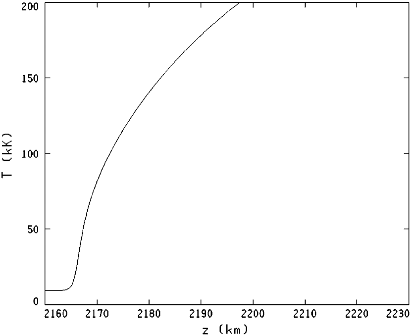
Figure 1: The temperature distribution used to determine the results shown in Figures 2 - 7 (modified version of model C from Fontenla et al. 1999).

Figure 1 shows part of the $T(z)$ distribution used in all three sets of calculations. This is essentially an extended version of the modified energy-balance static model C (Fontenla et al. 1999) based on FAL3 mentioned earlier. That model includes particle diffusion. Here we want to show the effects of flow without diffusion using this prescribed $T(z)$ distribution; hence the calculation in this section (like the equations shown in the previous section) omits the diffusion terms that are included in the determination of model C. Thus, the results given in this section are not realistic but are given for illustrative purposes only. This model extends up to coronal temperatures of $1.6\times 10^{6}$ K, but in Figure 1 we show only the low transition region where H and He are only partially ionized.

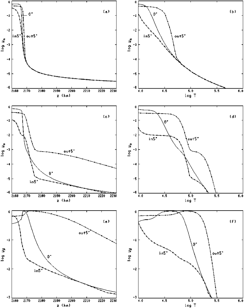
Figure 2: $y_{\rm a}$, $y_{\alpha}$, and $y_{\beta}$ vs. $z$ and vs. $T$ for models in5^′′, 0^′′, and out5^′′ without diffusion.

Figure 2a shows $y_{\rm a}(z)$ and Figure 2b shows $y_{\rm a}(T)$ for the three values of $F_{\rm H}$ considered here. These results show that outflow transports low-ionization material outwards while inflow transports high-ionization material inwards. In the former case, as the material travels into the high temperature region it becomes ionized by collisions with fast electrons. In the latter case the ionized material transported into the low temperature region recombines gradually.

Figures 2c and 2d show that $y_{\alpha}$ in the three cases has the same general behavior at lower temperatures as $y_{\rm a}$, but at higher temperatures $y_{\alpha}$ is almost 100 times larger for outflow than for inflow.

Figures 2e and 2f show $y_{\beta}$ in the three cases. In the outflow case, He is in the form of He II throughout a very extended region. The results show an enhancement of He II, relative to the static case, in the upper chromosphere for both outflow and inflow; also, the narrow maximum in He II at the base of the transition region in the static model disappears in both moving cases.

The results for He II are more complex than the others because outflows transport He II to higher temperatures but at the same time the ionization of He I transported from the chromosphere prevents He II depletion. Inward flow drives the He II and He III into the chromosphere where He III quickly recombines into He II, while He II recombines gradually.

We do not discuss these solutions further because they do not include diffusion. As noted at the beginning of this section, the purpose of these solutions is only to illustrate how velocity effects alone would affect the ionization balance.

4 Combined Flow and Diffusion

Now we consider the general case including the diffusion velocities, which were ignored in the preceding sections to simplify the discussion. The basic equations for the H and He diffusion velocities appear in FAL3, and here we restate some of them in summary form only. Again equation (13) is the basic equation and we use the same expressions as in §3 for $r$ and $s$. The transformation in equation (16) leading to equation (15) also can be carried out here. However, because $v_{ik}$ is not predefined but rather depends on the gradient of the ionization fraction, the analytic solution given by equation (18) is no longer possible. Thus, we replace $v_{ik}$ by explicit expressions derived from particle transfer theory (see FAL3, and also Braginskii 1965), and solve equation (13) numerically.

In general, the diffusion velocities can be expressed as linear functions of the logarithmic gradients of the “thermodynamic forces” (FAL1, 2, 3). This expression is

$$v_{ik}=\sum_{n}D_{ikn}Z_{n}\,,$$ (35)

where $D_{ikn}$ is the diffusion coefficient that expresses the dependence of the diffusion velocity of element $k$ in ionization stage $i$ on the thermodynamic force $Z_{n}$. In this paper we use the same expressions for $Z_{n}$ that we gave in FAL3 (see eqns. 15 and 16 in that paper) and we again neglect gravitational thermodynamic forces. As we did in our previous papers we express the relative diffusion velocities $u_{i,i+1,k}$ between consecutive ionization stages $i$ and $i+1$ of element $k$ as linear functions of the thermodynamic forces and then express the diffusion velocities $v_{ik}$ as linear functions of these relative diffusion velocities.

The definitions of the relative diffusion velocities as well as the expressions of the diffusion velocities in terms of the relative diffusion velocities are shown in FAL3 (see eqns. 14 and 17 in that paper). Although we solve the ionization equations in a slightly different way here, FAL3 gives the remaining details on the treatment of diffusion.

4.1 Hydrogen Flow and Diffusion

The ionization equilibrium equation (13) for H is

$${d\over dz}[y_{\rm a}(n_{\rm H}v_{\rm a}+F_{\rm H})]+ry_{\rm a}=s\,,$$ (36)

and using the derivations in FAL3 (mainly eqns. 16 and 17 in that paper) we can write

$$v_{\rm a}={x\over{1+x}}(d_{11}{{d\ln x}\over dz}+\Delta_{1})$$ (37)

where $x=n_{\rm p}/n_{\rm a}$, and

$$\Delta_{1}=d_{12}Z_{a}+d_{13}Z_{b}+d_{14}Z_{c}+d_{15}Z_{T}\,.$$ (38)

It can be shown without difficulty that

$$n_{\rm a}{x\over{1+x}}{{d\ln x}\over dz}=-n_{\rm H}{{dy_{\rm a}}\over dz}\,,$$ (39)

where $y_{\rm a}=n_{\rm a}/n_{\rm H}$ as before. Thus equation (36) becomes

$${d\over dz}(gy_{\rm a}-f{{dy_{\rm a}}\over dz})+ry_{\rm a}=s$$ (40)

where

$$f = d_{11}n_{\rm H}$$

$$g = F_{\rm H}+n_{\rm p}\Delta_{1}$$ (41)

and where $r$ and $s$ are given by equation (20). Appendix A gives the numerical method we use for solving the differential equation (40).

The solution of these equations is again iterated with the radiative transfer and statistical equilibrium equations for the level populations of hydrogen as described above, but now also including the hydrogen atom diffusion velocity $v_{\rm a}$ in the expression for $G_{m}$ for hydrogen level $m$ so that

$$G_{m}={1\over n_{m}}{d\over dz}[n_{m}(v_{\rm a}+{F_{\rm H}\over n_{\rm H}})]\,,$$ (42)

which replaces equation (25). Due to the large transition rates between bound levels, we assume that all the bound levels have the same diffusion velocity $v_{\rm a}$.

4.2 Helium Flow and Diffusion

The ionization equilibrium equations for He I and He II are

$${d\over dz}[y_{\alpha}(n_{\rm He}v_{\alpha}+F_{\rm He})]+r_{\alpha}y_{\alpha} = s_{\alpha}$$

$${d\over dz}[y_{\beta}(n_{\rm He}v_{\beta}+F_{\rm He})]+r_{\beta}y_{\beta} = s_{\beta}$$ (43)

Using the expressions for the diffusion velocities of neutral and ionized He, $v_{\alpha}$ and $v_{\beta}$, derived in FAL3, these diffusion velocities are written as linear functions of the thermodynamic forces and lead to the following equations:

$${d\over dz}[g_{\alpha}y_{\alpha}-f_{\alpha}{d\over dz}y_{\alpha}]+r_{\alpha}y_{\alpha} = s_{\alpha}$$

$${d\over dz}[g_{\beta}y_{\beta}-f_{\beta}{d\over dz}y_{\beta}]+r_{\beta}y_{\beta} = s_{\beta}$$ (44)

where as shown in Appendix B,

$$f_{\alpha} = n_{\rm He}\{(1+{y_{\gamma}\over y_{\beta}})[d_{33}(1-y_{\gamma})-d_{34}y_{\alpha}]+{y_{\gamma}\over y_{\beta}}[d_{43}(1-y_{\gamma})-d_{44}y_{\alpha}]\}$$

$$g_{\alpha} = F_{\rm He}+n_{\rm He}[(1-y_{\alpha})\Delta_{4}+y_{\gamma}\Delta_{5}]$$

$$f_{\beta} = n_{\rm He}\{d_{33}(1-y_{\gamma})-d_{34}y_{\alpha}-{y_{\gamma}\over y_{\alpha}}[d_{43}(1-y_{\gamma})-d_{44}y_{\alpha}]\}$$ (45)

$$g_{\beta} = F_{\rm He}+n_{\rm He}[y_{\gamma}\Delta_{7}-y_{\alpha}\Delta_{6}]$$

We again solve these equations using the numerical method described in Appendix A. Since the coefficients $f$ and $g$ depend on $y_{\alpha}$, $y_{\beta}$, and $y_{\gamma}$ we iterate between the solutions of equations (44) for $y_{\alpha}$ and $y_{\beta}$ until convergence is achieved. Also, as in §3, we iterate between the solutions of these equations and the radiative transfer and statistical equilibrium solutions for the bound levels of He I and He II, again introducing the diffusion velocities $v_{\alpha}$ and $v_{\beta}$ in the definitions of the corresponding $G_{m}$.

4.3 Flow and Diffusion Results

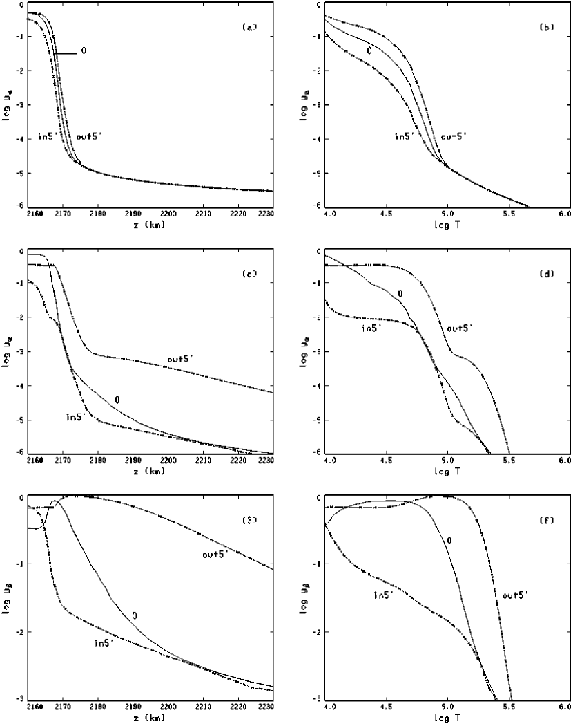
Figure 3: $y_{\rm a}$, $y_{\alpha}$, and $y_{\beta}$ vs. $z$ and vs. $T$ for models in5^′, 0, and out5^′ that include diffusion.

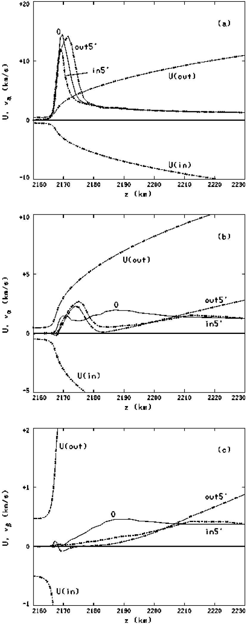
Figure 4: The flow velocity $U$, together with the H, He I, and He II diffusion velocities $v_{\rm a}$, $v_{\alpha}$, and $v_{\beta}$, respectively, for models in5^′, 0, and out5^′ that include diffusion.

We now show the calculated $y_{\rm a}$ distributions for the same $T(z)$ and the same set of three values of $F_{\rm H}$ (i.e., $+5\times 10^{15}$ [outward flow], 0 [zero flow], and $-5\times 10^{15}$ particles cm^-2 s^-1 [inward flow]) considered before but now including diffusion. We designate these models as out5^′, 0, and in5^′, respectively, using the single prime to indicate that these are models with the same prescribed temperature structure as before but now include diffusion. (Models 0^′′ and 0 are those without and with diffusion.) Figures 3a and 3b plot $y_{\rm a}$ vs. $z$ and $T$, respectively. Comparing Figures 2 and 3 shows that diffusion causes basic changes in the shape of the calculated curves in the lower transition region since (as shown in Fig. 4 below) the diffusion velocities are greater than the flow velocities near $z\sim 2170$ km.

Figures 3c-f show $y_{\alpha}$ and $y_{\beta}$ vs. $z$ and $T$. These He I and He II results do not differ greatly from those in Figure 2 without diffusion. Thus, for this $T(z)$ the effects of diffusion on the He ionization are not as important as in the case of H.

Our He II ionization equilibrium calculations include the effects of dielectronic recombination, based on rate coefficients given by Romanik (1988). Dielectronic recombination from He II to He I greatly exceeds radiative recombination for temperatures higher than $10^{5}$ K, and causes $y_{\alpha}$ to be more than ten times larger in this temperature range than would be calculated with radiative recombination alone.

Figure 4a shows both $U$ and the neutral hydrogen diffusion velocity $v_{\rm a}$ (eqn. 5) for the three cases. It is clear that in the lower transition region the H I diffusion velocity is larger than the absolute value of $U$ in all cases. Figures 4b and 4c show both $U$ and the diffusion velocities $v_{\alpha}$ and $v_{\beta}$ of He I and He II. For He I the diffusion velocity is smaller than $|U|$, although at some heights not by much. The difference from the H I behavior is in part due to the smaller logarithmic temperature gradient at the heights where the ionization of He I to He II occurs. The He II diffusion velocities shown in Figure 4c are much smaller than $|U|$ for a combination of reasons: because of the large momentum exchange between protons and both He II and He III; and because, at the heights where He II and He III occur, the proton diffusion velocity is small (since H is fully ionized there).

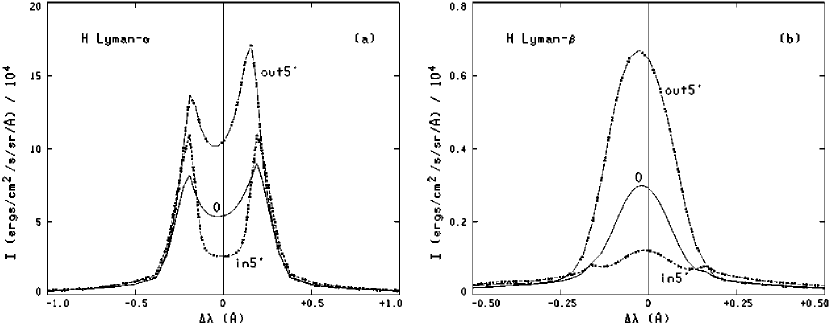
Figure 5: The calculated disk-center H line profiles for models in5^′, 0, and out5^′.

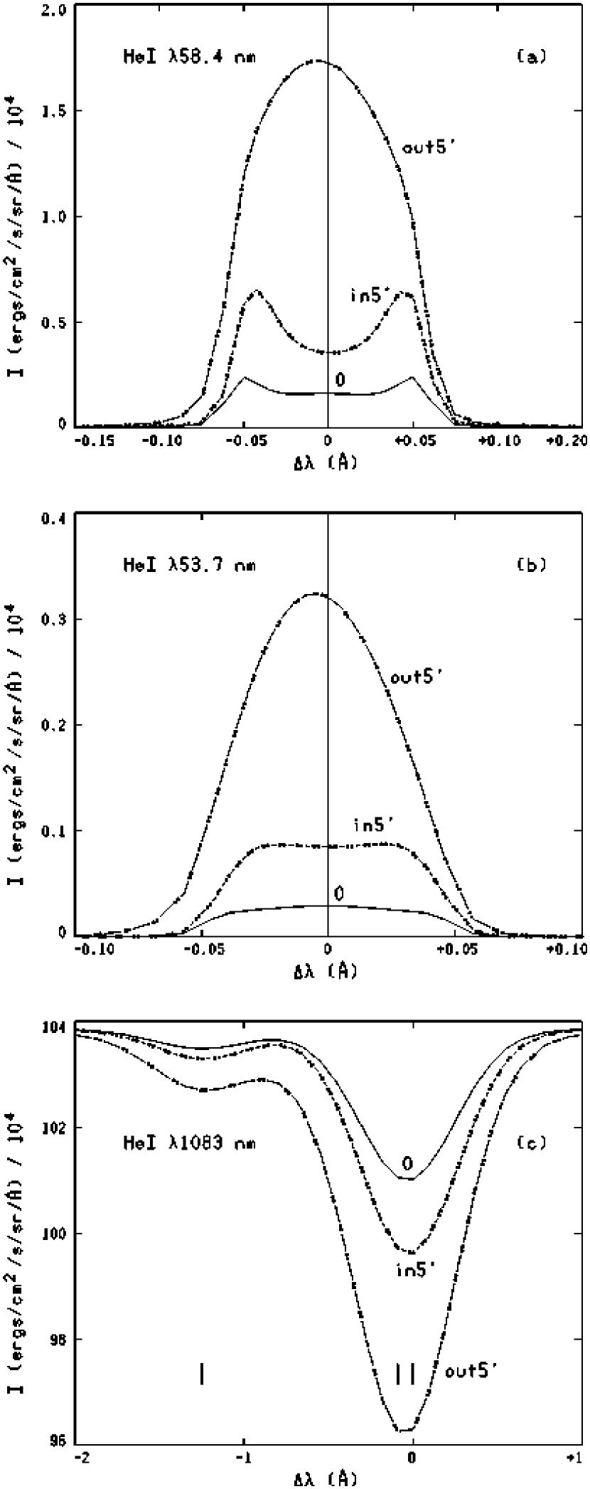
Figure 6: The calculated disk-center He I line profiles for models in5^′, 0, and out5^′.

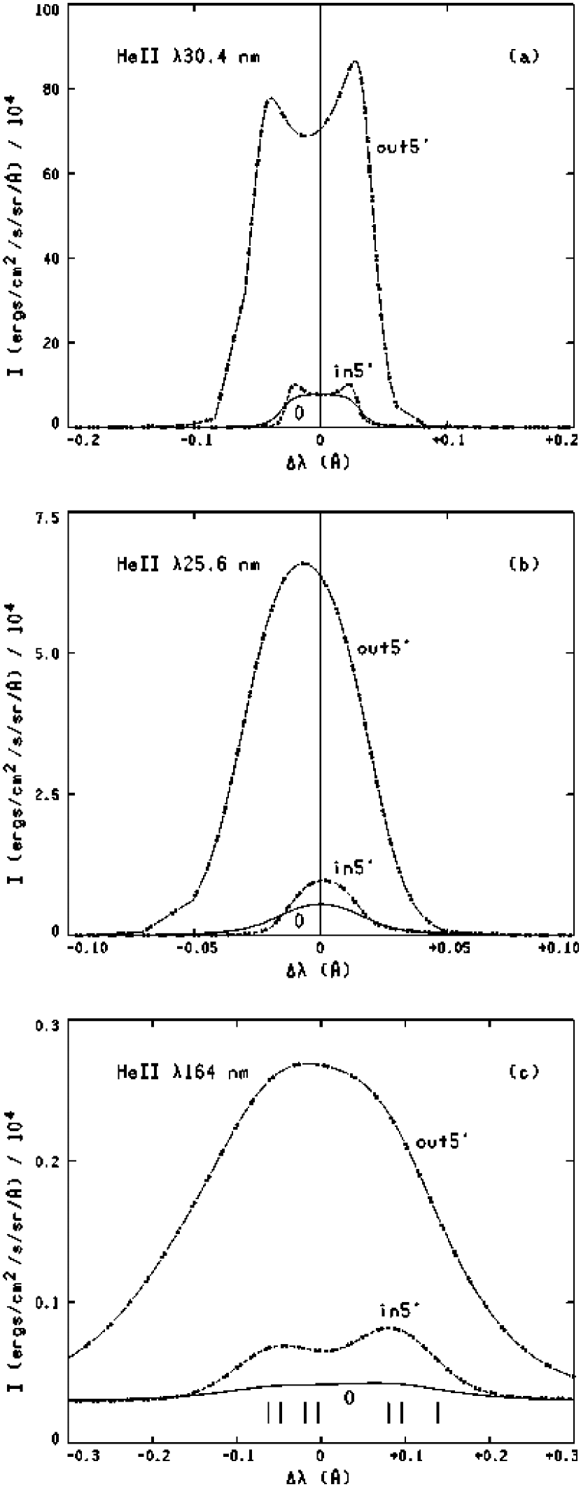
Figure 7: The calculated disk-center He II line profiles for models in5^′, 0, and out5^′.

Figure 5 shows the calculated H Lyman alpha and beta lines at disk center; Figure 6 shows the He I resonance lines at 58.4, 53.7, and 1083 nm; and Figure 7 shows the He II lines at 30.4, 25.6, and 164 nm. These figures show that mass flow produces very substantial changes in these line intensities and profiles far beyond the simple Doppler shifts, even in the cases considered here, which have same $T(z)$ distribution. The larger H line intensities in the outflow cases result from the enhanced neutral H at higher temperatures, producing greater radiative losses. The converse is true for inflows, although the Lyman $\alpha$ peaks, formed in the chromosphere, are enhanced.

Unit optical depth at the center of the He I $\lambda$ 58.4 nm line occurs at the base of the transition region near $z$ = 2160 km, where $T\approx 10^{4}$ K. Figure 3 shows that, in this region, the values of $y_{\alpha}$ for both in5^′ and out5^′ are smaller than in the static case and the values of $y_{\beta}$ for both in5^′ and out5^′ are larger than in the static case. The greater helium ionization in this region leads to enhanced He I line source functions. As Figures 6a and 6b show, this produces emission lines for both moving models that are stronger than in the static case. The greater He I ionization also increases the population of the lower level of the He I $\lambda$ 1083 nm line, thus causing greater absorption of the infrared photospheric continuum.

We return to a consideration of these calculated line profiles in §5 where we show the results for the energy-balance $T(z)$ distribution in each case.

5 Energy Balance

We now address the computation of self-consistent energy balance models of the transition region. Our methods are similar to those in our earlier papers but here we add the terms corresponding to the ionization energy and enthalpy transport due to the particle flows, $F_{\rm H}$ and $F_{\rm He}$, in addition to the corresponding terms due to the heat conduction and diffusion velocities already considered in our earlier papers.

As explained in Vernazza et al. (1981, §IX), we use the PANDORA computer program to compute the radiative losses due to H and He from the solutions of the equations shown above. These radiative losses now include the effects of flow as well as those of diffusion included in FAL3. To these radiative losses we add the free-free and other elemental radiative losses, using estimates based on the work of Cox and Tucker (1969). In the upper transition region radiative losses due to elements other than H and He dominate, and these estimates are only approximate since they do not take mass flow and particle diffusion into account. However, we consider our solutions to be accurate in the lower transition region, where losses due to H and He indeed greatly dominate. We will recompute the upper transition region of our models in a subsequent paper after obtaining better estimates of the radiative losses for elements other than H and He including the effects of particle diffusion and elemental flows.

After computing the total radiative loss, $q_{R}(z)$, we calculate $F_{R}(z)$, the integral of this quantity from the lower boundary of our energy balance calculation, $z_{0}$, out to the given height $z$ to obtain the inward energy flux at $z$ required to compensate for the radiative losses between $z_{0}$ and $z$.

As in FAL1, 2, and 3, we locate this lower boundary at the top of the chromosphere where the transition region is assumed to start. The height $z_{0}$ is obtained from observational constraints and cannot be derived from theory because it depends entirely on the details of chromospheric heating that are not yet well understood. Thus, the temperatures at heights below $z_{0}$ are those given by our semi-empirical model C described above. We compute the temperature stratification above $z_{0}$ by requiring that the downward heat transport balances the radiative losses (minus any mechanical dissipation, see below), or equivalently that the decrement of the total heat flux is equal to the value of $F_{R}$ mentioned above (minus any mechanical energy). The values of the height and temperature at our chosen boundary are $z_{0}$ = 2163.25 km and $T_{0}$ = 9530 K. Table 1 lists the full set of atmospheric parameters for the current version of model C used in the present paper. (This version differs slightly from the earlier one used by Fontenla et al. (1999) due the choice of $z_{0}$, the extension to higher temperatures, and to various improvements in the PANDORA calculations.)

Our method described here can take into account an ad hoc mechanical energy dissipation (or heating) term, $q_{M}$, that is assumed to have the form

$$q_{M}=C_{q}n_{\rm H}\,,$$ (46)

where $C_{q}$ is a coefficient chosen to account for this dissipation. This mechanical energy dissipation term is also integrated from the lowest boundary of our energy balance calculation, $z_{0}$, to obtain the mechanical energy flux, $F_{M}$, dissipated between the heights $z_{0}$ and $z$. However, we find that for the cases shown here, introducing $q_{M}$ as in equation (46), with the coefficient $C_{q}$ chosen in such a way as to compensate for the highly variable upper chromospheric radiative losses, has effects on lower transition region models that vary in each case. Here we want to show only the effects of velocity without introducing the further complication of variable mechanical heating since in many cases (inflows, the static case, and small outflows) a value of $C_{q}$ that would account for the upper chromospheric losses has no significant effect on the lower transition region. Thus, in this paper we have confined ourselves to cases with $C_{q}=0$. We do not include models with larger outflow in this paper because such cases indeed require much larger chromospheric heating which would have a significant effect on the lower transition region. In a later paper we will consider non-zero values of $C_{q}$ and show the effects of mechanical heating on the lower transition region, specially in cases of large outflow.

The total heat flux, $F_{h}$, is defined here as the sum of heat conduction, ionization energy transport and enthalpy transport terms as we show below. The energy balance requirement (from FAL2, eqs. 9-12) takes the form

$$F_{E}=F_{h}(z)+F_{R}(z)-F_{M}(z)$$ (47)

where $F_{E}$ is the constant value that results from the specified lower boundary condition, and is equivalent to the total heat flux at the lower boundary $z_{0}$. This energy balance equation is sometimes formulated by equating to zero the divergence of the right-hand-side of equation (47) (or the derivative with respect to $z$ in our one-dimensional modeling), which is equivalent to the integral form shown here.

The total heat flux $F_{h}$ can be expressed as

$$F_{h} = F_{T}+F_{U}\,,$$

$$F_{T} = -\kappa{{d\ln T}\over dz}+{5\over 2}n_{e}kTv_{e}+\sum_{i,k}n_{ik}({5\over 2}kT-E_{\rm ion})(v_{ik}+v_{k})\,,$$

$$F_{U} = {5\over 2}n_{e}kTU+\sum_{i,k}n_{ik}({5\over 2}kT-E_{\rm ion})U\,,$$

$$= {5\over 2}pU-U\sum_{i,k}n_{ik}E_{\rm ion}\,,$$

where $F_{T}$ is the thermally-driven heat flux, $F_{U}$ is the mass-flow-driven heat flux, $E_{\rm ion}$ is the ionization energy for element $k$ from ionization stage $i$ to the fully ionized stage, $\kappa$ is the coefficient of heat conduction, and the other symbols have their previous meaning. (Note that for the heat conduction we use not the plain gradient of the temperature but the logarithmic temperature gradient.) In these equations we use the condition of zero electric current that determines the electron diffusion velocity $v_{e}$ to be the same as the sum of the diffusion velocities of all hydrogen and helium ions weighted by their charge. Since we apply these equations at heights above the chromosphere, the ions of elements other than H and He can be neglected for the purpose of computing $v_{e}$. The zero electric current condition leads to a “thermoelectric” field (see MacNeice, Fontenla, & Ljepojevic 1991), which is implicitly included in all our calculations. The terms in $F_{h}$ that contain $E_{\rm ion}$ are called “reactive heat flux” terms; those in $F_{T}$ are thermally driven, and those in $F_{U}$ velocity driven.

The equations for $F_{T}$ and $F_{U}$ can be elaborated using the definitions of $v_{e}$ and the mass flow $F_{m}$, so that

$$F_{T}=F_{\rm cond}+{5\over 2}kT\sum_{i,k}n_{ik}(v_{ik}+v_{k})q_{i}+{5\over 2}kT\sum_{k}n_{k}v_{k}+F_{T{\rm react}}\,,$$ (49)

where $F_{\rm cond}=-\kappa d\ln T/dz$ is the conductive heat flux, $q_{i}$ is the electric charge of the ionization stage $i$, and where

$$F_{T{\rm react}}=-\sum_{i,k}n_{ik}E_{\rm ion}(v_{ik}+v_{k})$$ (50)

is the thermally-driven reactive heat flux; and

$$F_{U}={5\over 2}{p\over\rho}F_{m}+F_{U{\rm react}}\,,$$ (51)

where

$$F_{U{\rm react}}=-U\sum_{i,k}n_{ik}E_{\rm ion}=-(F_{m}/\rho)\sum_{i,k}n_{ik}E_{\rm ion}\,,$$ (52)

is the velocity-driven reactive heat flux.

Our method for determining the temperature structure using the energy balance equation (47) assumes that the thermally-driven heat flux $F_{T}$ can be expressed as a coefficient times the logarithmic temperature gradient. This is plainly true for the heat conduction term and is approximately true for the other terms because they depend on the diffusion velocities. The diffusion velocities are also driven by the temperature gradient: directly in the case of thermal diffusion, and indirectly in the case of ionization gradients. Thus in the transition region the dependence of the thermal heat flux $F_{T}$ on temperature can be described by

$$F_{T}=-K(z){{d\ln T}\over dz}$$ (53)

where the coefficient $K$ is obtained by dividing $F_{T}$ (computed in detail from the equation 49) by the logarithmic temperature gradient. In our earlier papers we called $K$ the “effective” heat transport coefficient.

The first term in equation (51) for $F_{U}$ varies because the ratio of gas pressure to mass density, related to the sound speed, varies as the temperature changes; however, the second term has a stronger variation because it depends on the H and He ionization changes. Although these variations are due to the temperature variation, $F_{U}$ cannot be expressed as a linear function of the logarithmic temperature gradient. We take $F_{U}$ as given in our procedure for correcting the height scale and recompute it in each iteration of the overall procedure.

After computing the radiative losses, energy fluxes, $K$, and $F_{U}$, we adjust the position of each point of our height grid, stretching or compressing the intervals between adjacent points in such a way that equation (47) is satisfied at all heights in the transition region. For this, we start at $z_{0}$ and step outwards, recomputing the position of each height point so that the height interval from the adjacent lower point, $\Delta z$, satisfies the following equation

$$-K_{i-1/2}{{\Delta\ln T}\over\Delta z}+{F_{U}}_{i-1/2}=F_{E}-(F_{R}-F_{M})_{i}-{{\Delta z}\over 2}(q_{R}-q_{M})_{i-1/2}$$ (54)

where the index $i$ is that of the lower point of the interval in question, and the values with the index $i-1/2$ are the mean values of that interval. Note that the sum of the terms on the right hand side is equal to $F_{E}-(F_{R}-F_{M})_{i-1/2}$, and that the sum of the terms on the left hand side is $(F_{h})_{i-1/2}$. Thus, this equation is a numerical approximation of equation (47) evaluated at the center of the interval. As the calculation proceeds outward to the next interval, the value of $(F_{R}-F_{M})_{i-1}$ is recomputed incrementally,

$$(F_{R}-F_{M})_{i-1}=(F_{R}-F_{M})_{i}+\Delta z(q_{R}-q_{M})_{i-1/2}\,.$$ (55)

Equation (54) is quadratic in $\Delta z$; in solving it we select the sign of the square root term in the solution so that $\Delta z$ is positive, which often implies that a different sign must be chosen depending on the sign of $F_{U}$. We avoid the numerical cancellations which can arise when the velocities are large, or near zero, and use an asymptotic expression in such situations.

This scheme for computing a revised height grid is nested in a procedure consisting of the following steps: compute corrections for $\Delta z$; apply damping to the computed corrections; construct the revised height grid; and, recompute the fluxes using the same $K$, $F_{U}$, $q_{R}$, and $q_{M}$. This height grid revision procedure is iterated a few times.

Then, we recompute the ionization and the non-LTE radiative transfer equation as described in the earlier sections. We recompute the radiative losses, energy fluxes, and the coefficient $K$, and solve equation (54) again as described above. This procedure converges rapidly and has the virtue of simplicity, since the “effective heat transport coefficient” $K$ hides the complicated dependencies on the temperature gradient. This method has served us well in building a grid of models incrementally, enabling us to start the computation of a new model by using another one with a different particle flux.

6 Effects of Velocities in the Self-Consistent Models

We now discuss the results obtained for a set of models illustrating six cases of hydrogen particle flow, $F_{H}$: outflows $+2\times 10^{15}$ and $+1\times 10^{15}$ particles cm^-2 s^-1; zero flow; and inflows of $-1\times 10^{15}$, $-5\times 10^{15}$, and $-10\times 10^{15}$ particles cm^-2 s^-1. We refer to this sequence of six models by the names out2, out1, 0, in1, in5, and in10, respectively. Table 2 shows the logarithmic gradients of $T$ and $n_{\rm p}/n_{\rm a}$ at two temperature values, $2\times 10^{4}$ and $10^{5}$ K.

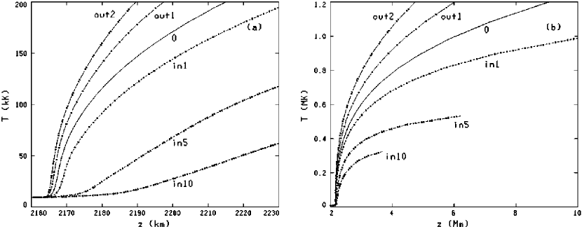
Figure 8: The calculated temperature distributions (a) in the lower transition region, and (b) extending into the corona, for the six energy-balance models out2, out1, 0, in1, in5, and in10. The upper temperature limits are chosen to keep the flow velocities subsonic.

Figure 8a shows the calculated $T(z)$ structures in the low transition region, and Figure 8b shows the $T(z)$ structures at greater heights in the upper transition region and the low corona. Clearly, the flow velocities considered here strongly affect the energy-balance temperature structure throughout the transition region and low corona.

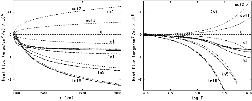
Figure 9: The total heat flux $F_{h}$ (curves with dots and short and long dashes as in Fig. 8) and its velocity-driven component $F_{U}$ (dashed curves), from equation (48), vs. $z$ and vs. $T$.

Inflows lead to much smaller temperature gradients due to the much smaller need (or no need) of thermally-driven heat transport to support radiative losses. Large inflow velocities lead to an extremely extended transition region in which the variation in energy transported down by the mass flow through each large height interval is dissipated by the radiative losses in that interval. At such shallow temperature gradients the thermally-driven heat flux $F_{T}$ is negligible. (Fig. 9, below, illustrates this behavior.)

The opposite is true for outflows. The temperature gradient must increase as the outward mass flow increases so that the inward thermally-driven heat transport variation can compensate for the large velocity-driven outward energy flow variation and the radiative losses.

Note that our statements regarding $T(z)$ apply only to the transition region and lower corona. In coronal layers above those considered here the effect of mechanical dissipation becomes very important, and the effects of velocity reverse themselves at heights beyond the temperature maximum in the corona because then the energy flow by particle outflows has a direction opposite to that of the temperature gradient. Thus outflows cause a thinner transition region with the corona closer to the chromosphere, but then a more extended high corona where the temperature is over a million degrees. Of course this is true only if the boundary condition at the top of the chromosphere remains the same and the coronal heating increases accordingly.

Figure 9 shows the total heat flux, $F_{h}$, and its velocity-driven component, $F_{U}$ (see equation 48). For outflows, $F_{U}$ is large and positive but, due to the very steep temperature gradient, it is overpowered by $F_{T}$ in the very thin transition region. For small flow velocities (out2 to in1), the total heat flux is almost the same at temperatures below about $10^{5}$ K, and is about $-2\times 10^{5}$ ergs cm² s^-1 at that temperature, regardless of $F_{U}$ (which has the same sign as the particle flow). For large inflows the curves diverge, and the heat flux at $10^{5}$ K for the in10 case is about four times larger (in absolute value) than for small flows.

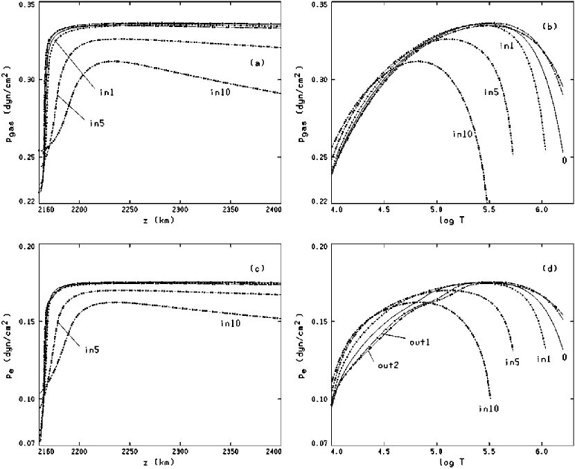
Figure 10: $p_{\rm gas}$ and $p_{e}$ vs. $z$ and vs. $T$.

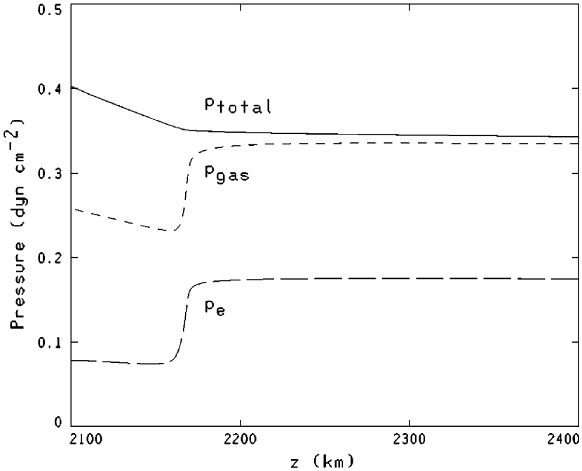
Figure 11: $p_{e}$, $p_{\rm gas}$ and $p_{\rm total}$ vs. $z$ for model in1.

Figure 10 shows the gas pressure and electron pressure contributions in the models. In the chromosphere, the gas pressure has a more gradual decrease than would be expected in hydrostatic equilibrium without the turbulent pressure term (see equation 34). The gas and electron pressures reach a local minimum at the top of the chromosphere below the abrupt increase caused by the temperature increase (that overpowers the density decrease) in the transition region. The “total pressure” $p_{\rm total}$ in equation (34) decreases monotonically with height, as shown in Figure 11 for the in1 model.

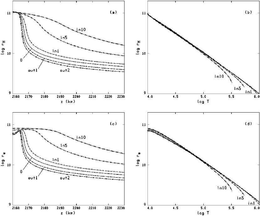
Figure 12: $n_{\rm H}$ and $n_{e}$ vs. $z$ and vs. $T$.

Figures 12a and 12c show $n_{\rm H}$ and $n_{\rm e}$ as functions of height for all the models. The differences between these curves are mainly due to the different $T(z)$ structures of the models. As shown in Figures 12b and 12d, $n_{\rm H}$ and $n_{\rm e}$ as function of $T$ are about the same for all the models except near the upper boundary where the flow approaches the sound speed.

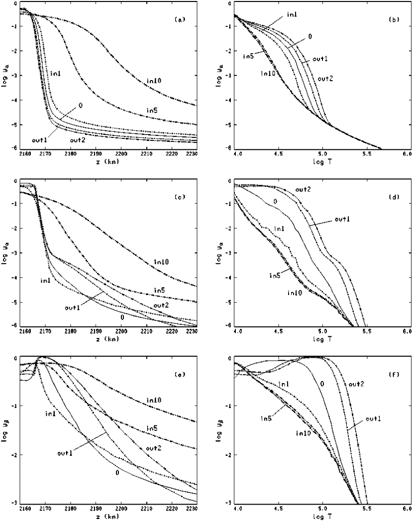
Figure 13: $y_{\rm a}$, $y_{\alpha}$, and $y_{\beta}$ vs. $z$ and vs. $T$.

Figures 13a and 13b show the neutral hydrogen fraction, $y_{\rm a}$, as functions of $z$ and $T$. The variation of $y_{\rm a}(T)$ for $T$ greater than $\approx 4\times 10^{4}$ K in Figure 13b resembles the curves shown in Figure 3b for models that all use the same $T(z)$ structure as the static case here. Thus, the changes in $y_{\rm a}(T)$ due to mass flows above the region of Lyman $\alpha$ formation are not much affected by the temperature structure. However, at lower temperatures the curves in Figure 13b all tend to converge, while those in Figure 3b remain well separated, even at $10^{4}$ K. This is because the back-radiation in the energy balance cases is less affected by the flow (as we show below) than in cases where the temperature structure was prescribed. For the large inflows in Figure 13b diffusion becomes negligible and $y_{\rm a}$ depends only on temperature.

The relationship between Figure 13a and Figure 3a is more complicated because Figure 13a combines the effects of both the changing temperature gradient and the velocities. Figure 8 shows that the temperature at a given height is smaller for inflows than for outflows, e.g., at $z$ = 2170 km, $T$ = 41200 K for in1 and $T$ = 81800 K for out1. As a result $y_{\rm a}$ at this height is larger for inflows than for outflows since hydrogen is not as highly ionized. This contrasts with the results in Figure 3a, based on a common $T(z)$, where $y_{\rm a}$ at a given height is smaller for inflows than for outflows.

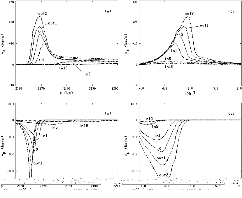
Figure 14: $v_{\rm a}$ and $v_{\rm p}$ vs. $z$ and vs. $T$.

Figure 14 shows the total diffusion velocities of H atoms and ions (protons), $(v_{\rm a}+v_{\rm H})=V_{\rm a}$ and $(v_{\rm p}+v_{\rm H})=V_{\rm p}$ (but note that we assume no relative diffusion velocities between H and He, so that $v_{\rm H}=v_{\rm He}=0$). These velocities are substantial for the outflow and the static models; they are still significant for the inflow model in1, but are negligible for in5 and in10 since the temperature and ionization gradients are very small in these cases.

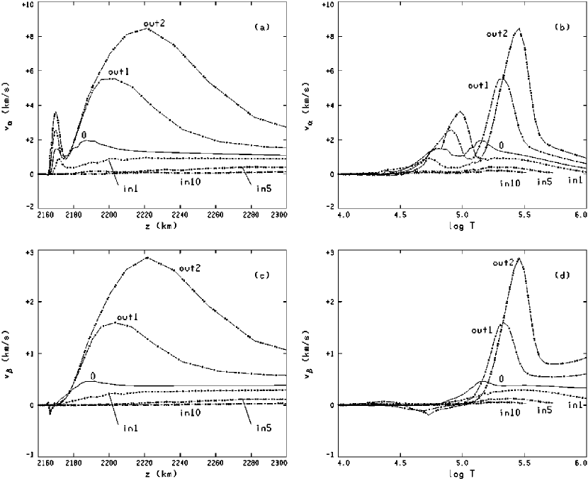
Figure 15: $v_{\alpha}$ and $v_{\beta}$ vs. $z$ and vs. $T$.

Figure 15 shows the helium diffusion velocities $v_{\alpha}$ and $v_{\beta}$. Comparison with Figures 4b and 4c (for $T(z)$ prescribed) shows that the diffusion velocities are now different because the changes in $T(z)$ tend to increase He diffusion for outflows, and to decrease it for inflows.

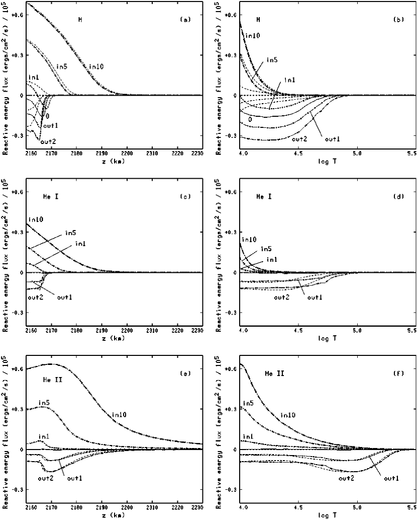
Figure 16: The H, He I, and He II components of $F_{U{\rm react}}$ (dashed curves) and $F_{\rm react.total}$ (curves with dots and short and long dashes as in Fig. 8), vs. $z$ and vs. $T$. See equations (50), (52), and (56).

Figure 16 shows the reactive components of the energy flow (see §5) pertaining to H and He ionization energy transport. We show $F_{U{\rm react}}$ from equation (52) (dashed lines) due to the mass flow alone, and the sum

$$F_{\rm react.total}=F_{U{\rm react}}+F_{T{\rm react}}$$ (56)

representing the “total reactive energy flow” which includes both mass velocity and particle diffusion effects. Figures 16a and 16b show these quantities for H as function of $z$ and $T$, respectively. These figures show that for H the temperature-driven part (due to diffusion) dominates in the outflow models, static models, and for in1, but is small for in5 and negligible for in10. The particle diffusion effect is much less important for He I as shown in Figures 16c and 16d, and it is negligible for He II (Figures 16e and 16f). The He temperature-driven reactive energy flux is negligible in most cases (except for the static model) because it is overbalanced by the He II reactive velocity-driven energy flux.

The temperature-driven H reactive energy flux plays a major role in the low transition region of all the models except in5 and in10. The values of $F_{U{\rm react}}$ and $F_{\rm react.total}$ are shown in Table 3 for $2\times 10^{4}$ K, and in Table 4 for $10^{5}$ K. These tables also list the values of $F_{h}$ and $F_{\rm cond}$ (eqns. 48 and 49) and the height above $z_{0}$, the base of the transition region, in each model. In the large inflow cases the enthalpy energy flow becomes dominant and so large that radiative losses are only able to dissipate this energy within a layer of large extent. This leads to very shallow temperature gradients and to very extended transition regions in these cases.

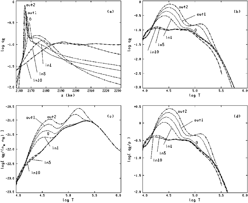
Figure 17: $q_{R}$ vs. $z$ and vs. $T$; $q_{R}/{n_{\rm e}n_{\rm H}}$ vs. $T$; and $q_{R}/p$ vs. $T$.

Figure 17 shows the total radiative losses $q_{R}$ as functions of $z$ and $T$. Figure 17a shows that in most cases these radiative losses are sharply peaked in the transition region, but this peak shifts to greater heights, and broadens, for inflows. The opposite is true for outflows. Figure 17b shows that the large inflow cases practically share a common curve (except for some departure at high temperature) and have a very flat maximum. In models with small inflow and with outflow the H and He peaks become bigger and shift to larger temperatures as the flow increases; this behavior is typical of the effects of particle diffusion. Also, we note that at temperatures near $10^{4}$ K the large inflow models, due to the H contribution, have larger radiative losses than all the others, but these radiative losses are not very large in absolute value.

Figures 17c and 17d show the radiative losses scaled differently, in ways commonly used in the literature. They show the same basic behavior as 17b. At temperatures above $4\times 10^{5}$ K the radiative losses shown in Figure 17c are almost the same for all models, but this is just due to our assumption that the function $q/{n_{\rm e}n_{\rm H}}$ as defined by Cox & Tucker (1969) accounts for the radiative losses due to all elements other than H and He. This assumption is probably not accurate because diffusion and flows would produce the same effects on other species (although if these are ionized the diffusion effects are probably small). At lower temperatures where the H and He radiative losses dominate, these functions are different for all the models, thus showing that none of the customary scaling laws applies for cases with flows. A different case is that of large inflows for which Figures 17 show that the radiative loss follows a common curve.

7 Line Profiles

In this paper we are not concerned with fitting any particular observations but only with showing the physical effects of the combined diffusion and mass flow processes on the H and He ionization and line formation. We do not show models of active regions or other specific solar features. These are postponed to a later paper where we include mechanical energy dissipation which, for simplicity, is not included here. Given these limitations, we note how our results compare with available observations of high spectral, temporal, and spatial resolution, to indicate where our results are generally consistent with the behavior of observed lines, and to show where some problems still remain.

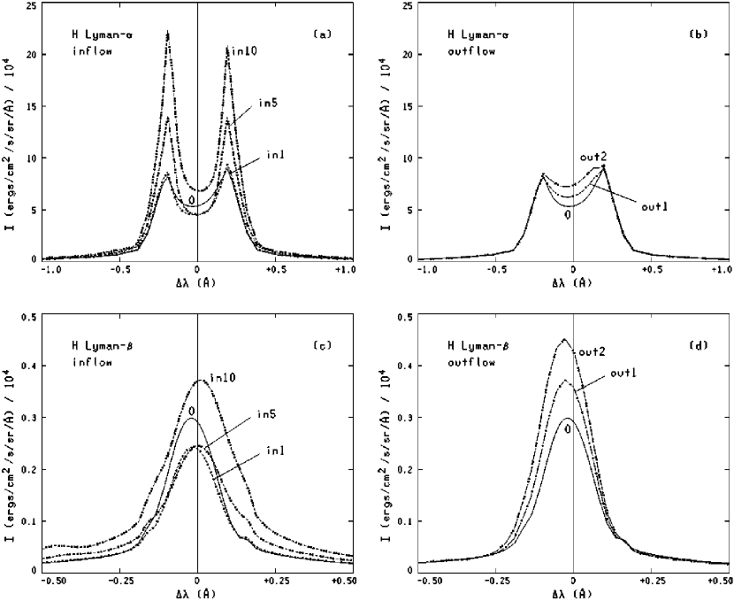
Figure 18: The calculated disk-center H line profiles for the six energy-balance models.

Figures 18a and 18b show the Lyman-$\alpha$ profiles for the inflow and outflow cases, respectively. In the inflow cases the lines become slightly broader and the peak intensities increase with increasing flow, producing an increase in the integrated line intensity, but asymmetries only start to become substantial for large inflows (for in10 the blue peak is larger than the red peak). For inflows the central intensity increases less than the peaks do and this leads to a larger relative central reversal where the peak-to-center ratio may reach $\sim 4$. In the outflow cases the peak intensities increase very little but the central intensity increases with increasing flow (thus also producing an increase in the integrated intensity, but for a different reason). For outflows the relative central reversal becomes smaller and the peak-to-center ratio may drop as low as 1.2. For outflows the asymmetry remains small and manifests itself as a slight increase of the red peak as the deepest point of the central reversal moves very slightly to the blue. This asymmetry is so small that it may be hard to detect in observations.

These changes in line profiles arise for different reasons in inflows and in outflows. For inflows the diffusion effects become smaller as the flow increases, and for large inflows become insignificant. This drives the region of formation of the line center deeper in the atmosphere where the temperature is lower than in the static case but where the line source function is enhanced because the electron density is higher, thus producing a moderate decrease at line center, except for model in10 where there is a moderate increase at line center. The peaks form at the top of the chromosphere (at $\sim 10^{4}$ K or less) where diffusion effects are small in all cases; thus, the increased peak intensities are just due to the larger electron density and amount of material at this temperature. For outflows, on the other hand, diffusion effects increase and shift the region of formation of line center to a layer which is thinner but has temperatures of $\sim 3\times 10^{4}$ K or more, while the line peaks still form at about the same temperature and electron density as in the static case.

This behavior of the computed Lyman-$\alpha$ line is consistent with the very detailed observations by Fontenla, Reichmann, & Tandberg-Hansen (1988, hereafter FRT), who found that the relative depth of the central reversal of this line changes with position (unfortunately, appropriate time sequences were not available). While the average quiet Sun profile and absolute intensity are in reasonable agreement with the static models (see FAL1), FRT showed that some quiet Sun profiles have deeper and others have shallower central reversals than the average. This effect is larger in active regions where intense peaks are sometimes observed at some locations, while at other locations in active regions the central reversal of the line is almost filled in. Of course in active regions the line is generally more intense (see FRT and FAL3) since their chromospheric temperature, and heating, are larger. Regardless of these intensity differences, the processes described here, whereby the the peak-to-center ratio grows larger with inflows and decreases with outflows, appear to be consistent with observations. (For example, Fig. 6 of FRT shows two profiles whose central reversals are very different, and in Fig. 8 of FRT the inflow profile c has a much deeper reversal than the outflow profiles b and d.)

Figures 18c and 18d show the Lyman-$\beta$ profiles for the inflow and outflow cases, respectively. The outflow profiles (Fig. 18d) show increasing intensity as the flow increases. This is again due the increased effects of diffusion that drive the line center formation region up to temperatures of $\sim 3\times 10^{4}$ K; the effect of this higher temperature overpowers the reduction in the thickness of the region of line formation. The inflow profiles (Fig. 18c), instead, show a slight decrease of intensity for small inflows due to the shift of the line center formation region toward lower temperatures because of the reduction of diffusion effects. With large inflows the line becomes stronger and wider than in the static case due to the increasing optical thickness of the line-emitting region. There are no pronounced asymmetries but clearly the line center is shifted slightly to the red with inflows and to the blue in the static case, while the outflow cases show increasing blue shift.

The Lyman-$\beta$ line profiles observed by SOHO (Warren, Mariska & Wilhelm 1998) show a peak intensity of $\sim 2000$ erg cm^-2 s^-1 sr^-1 Å^-1 and integrated intensity of $\sim 900$ erg cm^-2 s^-1 sr^-1 (or $\sim 800$ when the local continuum is removed), and these values are consistent with our current static model. However, the Lyman-$\beta$ profile observed by SOHO shows a very small but definite asymmetric self-reversal that is not predicted by our present static calculations. This small central reversal contrasts with larger ones reported previously from OSO 8 data; however, the large reversals observed by OSO 8 may have been caused by geocoronal absorption, given the low orbit of that spacecraft. The relatively low spectral resolution of these data makes it difficult to separate the geocoronal absorption in the way used by FRT for Lyman-$\alpha$ line profiles. In the context of our models, several possibilities remain to account for the small Lyman-$\beta$ central reversal observed by SOHO. 1) One likely possibility suggested by FRT and by Fontenla, Fillipowski, Tandberg-Hansen, & Reichmann (1989) is absorption by a “cloud layer” consisting of H I dynamic material in the lower corona just above the transition region. The spicules observed in H$\alpha$ are the densest component of such a layer but, of course, much more material is visible at the limb in Lyman-$\alpha$ than in H$\alpha$, and all this material would absorb in Lyman-$\beta$. 2) Another likely possibility is that portions of the disk are covered by regions of inflow, of outflow, and of stationary material, and that a combination of our computed profiles in these cases may produce an apparent self-reversal. 3) It is possible that an unknown blend may cause an apparent self-reversal. However, all higher Lyman lines show a similar, but decreasing, asymmetric self-reversal and this is hard to explain by a blend unless it involves a series analogous to the Lyman series. Consequently we consider a blend near line center of Lyman-$\beta$ only a remote possibility. Note that any of the above possible explanations also may account for the asymmetry of the central reversal and its evolution among the higher members of the Lyman series.

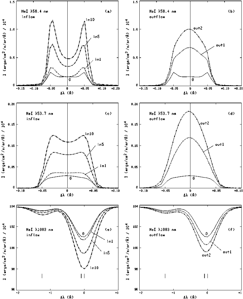
Figure 19: The calculated disk-center He I line profiles for the six energy-balance models.

The He I line profiles are shown in Figure 19. The behavior of the resonance line with the lowest excited level energy, the 58.4 nm line, is somewhat similar to that of Lyman $\alpha$. With increasing inflow the self-reversal becomes more pronounced because the peaks increase more than the line center. However, in contrast with Lyman $\alpha$, with increasing outflow the line center increases very strongly and changes the line’s shape from self-reversed to almost pure emission (for out2). The 53.7 nm line behaves similarly; however, 1) it does not have a self-reversal in the static case but a flat top instead, and 2) it develops only a moderate self-reversal with increasing inflow. The infrared absorption line at 108.3 nm deepens with the magnitude of the flow velocity. This strengthened absorption is mainly due to increased optical thickness: for inflows, this is caused by the greater extent of the lower transition region; for outflows, this occurs at the top of the chromosphere where increased UV radiation enhances the population of the triplet ground level due to greater He II recombination (see FAL3 and Avrett, Fontenla, & Loeser (1994) for a discussion of how this line is formed).

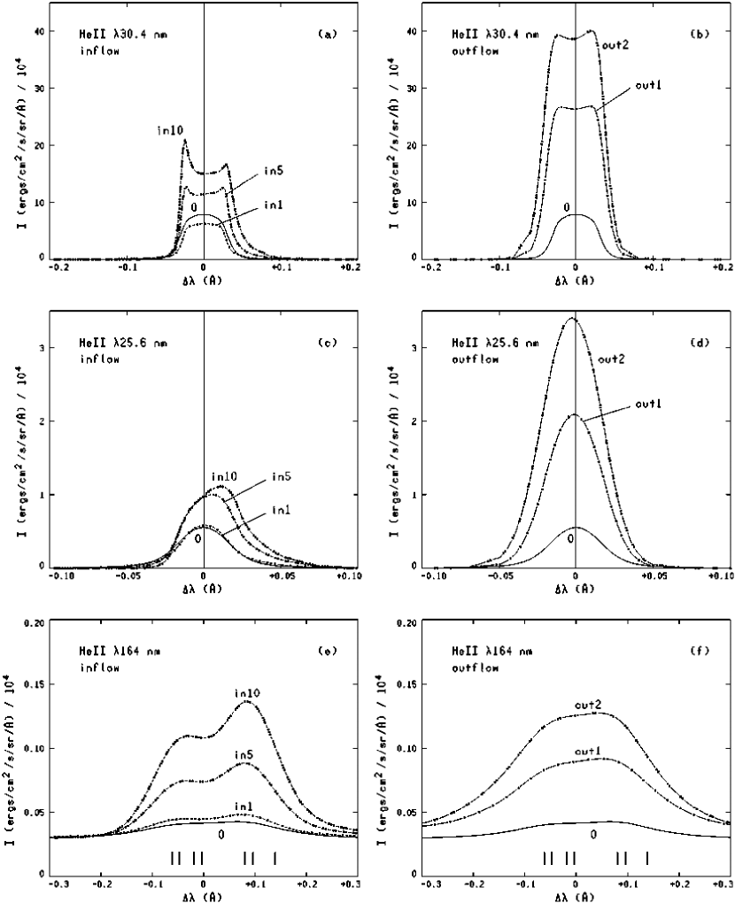
Figure 20: The calculated disk-center He II line profiles for the six energy-balance models.

The He II lines shown in Figure 20 behave differently from the H and He I lines. However, their intensities still increase with increasing flow velocity, regardless of its sign, except in the case of model in1. The lowest excitation resonance line, at 30.4 nm, has a flat top in the static case and develops a small self-reversal as the magnitude of the flow velocity increases. For inflows this occurs because, with increasing velocity, the line-center-forming region grows thicker geometrically and moves to lower temperature and higher electron density. For outflows the line intensity increases strongly because the line-forming region occurs at higher temperatures and this more than compensates for the smaller optical depth.

The He II 25.6 nm line also grows stronger with both increasing inflows and increasing outflows, and becomes rather bright for outflows. This line has a typical pure emission profile in all cases. Its center shifts appreciably (even more than Ly $\beta$) since this line forms at greater heights where velocities are larger.

The He II 164.0 nm line grows stronger with both increasing inflows and increasing outflows, but the line shape is flatter for outflows. There are differences between our computed profiles and observations (e.g., Kohl 1977): in our calculations the composite red peak is somewhat larger than the composite blue peak, while the opposite is generally observed. Walhstrom & Carlsson (1994) calculated the 164.0 nm line using model C of Vernazza et al. (1981) without diffusion or velocities. They found that the collisional coupling between the three n = 2, as well as the five n = 3 fine-structure levels, at transition region densities, is not large enough to populate each group according to their statistical weights, and that this results in changes in the shape of the composite 164.0 nm line that lead to closer agreement with the observations. In the present paper, however, we have assumed for simplicity that the two groups of sublevels are populated according to their statistical weights, and this may be the reason for the discrepancy with the observations. Also, since this composite line is broad, comparison with observations must consider blends with other lines, e.g. Cr II 164.0364 nm, Fe IV 164.037 nm, Fe III 164.0384 nm, and possibly other identified lines, that may blend into the composite red peak.

Our calculations show that, for the moderate flow velocities we consider here, line shifts are so small that they might only be detectable in the relatively weak Lyman-$\beta$ line and the somewhat stronger He II 25.6 nm line. For the largest inflows, our computed blue peaks of the bright and saturated or self-reversed resonance lines of H and He are brighter than the red peaks. However, for small flows both computed peaks are nearly equal and the differences would be undetectable. Consequently the line shift and asymmetry of these bright lines would not be practical diagnostics of small flows. Rather, the magnitude of their self-reversal, and their relative intensities, would be better diagnostic tools.

8 Discussion

The present paper differs from the work of CYP in that they do not include the effects of particle diffusion and velocities in the calculations of H and He ionization. Consequently their calculated level populations and radiative losses also are not consistent. Instead, they use values of the ionization and radiative losses from a previous paper by Kuin and Poland (1991) that does not include particle diffusion or flow velocities. As a result, although the CYP paper is an improvement over previous work that did not consider partial ionization or optically thick radiative losses, it does not present results from consistent calculations such as the ones we show here. Despite these shortcomings, CYP provides the correct qualitative behavior (like earlier papers) in that downflows smooth the temperature gradient while upflows sharpen it. Quantitatively, however, most of their results are very different from ours.

The radiative losses presented by Kuin and Poland and used by CYP consider radiative transfer effects in a static case but greatly underestimate the H and He radiative losses because they ignore particle diffusion. As explained in the FAL papers, particle diffusion produces larger H and He losses than those shown by CYP in their Fig. 1, and these losses occur at higher temperatures than where these elements emit their line radiation in models ignoring diffusion. Also, as explained in the FAL papers, our computed absolute Lyman-$\alpha$ profile is consistent with observations while calculations like those of Kuin and Poland do not give radiative losses large enough to correspond to the observed emission in the core of the Lyman-$\alpha$ line because they do not include particle diffusion.

Furthermore, the consistent calculations shown here demonstrate that the H and He radiative losses are influenced by the flows. This is easily seen when comparing Fig. 1 of CYP with Fig. 17 of this paper. In our present calculations the radiative losses for various flows (at comparable temperatures) differ substantially from each other except for large downflows. We have shown that this greatly affects the energy-balance $T(z)$ stratification and the values of the various components of the heat flux.

Similar considerations apply to the H and He ionization. As explained in the FAL papers, particle diffusion has an important effect on the ionization which is not considered by Kuin and Poland and consequently not by CYP. This is closely related to the statements above about the radiative losses and we refer the reader to the FAL papers for details. Also, particle flows have large effects on the ionization and these are ignored by CYP. Because of the different ionization, the reactive heat transport is different in our models than in those of CYP.

The net result of all this is that in many cases our $T(z)$ distributions are much shallower that those of CYP, and that our values of the contributions to the heat flux differ from theirs. Since these two calculations use different boundary conditions and different underlying chromospheres and photosphere, we do not give detailed numerical comparisons; but comparisons of their plots and ours show evident differences.

The boundary parameters at the base of our calculation of the transition region are: density, temperature, H and He ionization, He abundance, temperature gradient, H and He ionization gradients, H and He particle flows, and turbulent pressure. Magnetic topology can be added when a magnetic field structure more complicated than a vertical magnetic field is considered. The boundary parameters we use are all at the top of the chromosphere. In principle we could instead choose to specify these parameters at the coronal boundary. While boundary conditions can be prescribed in many ways, it is often easier to compute models by fixing them at just one of the boundaries. The results obtained in this way, then, define the values of the parameters at the other boundary. Thus one can adjust the prescribed chromospheric boundary conditions to match coronal observations as well.

We compute the energy balance only in the transition region, where we assume that radiative losses are balanced mainly by the total heat flux from the corona (including the ionization energy flow, also called reactive heat flow) and by the enthalpy flow (outward or inward, depending on the particle flow). Note that the radiative losses (expressed per unit volume, unit mass, or any other usual form—see Fig. 17) in the transition region are orders of magnitude larger than those in the underlying chromosphere or the overlying corona. Thus if one assumes that the mechanical energy dissipation in the transition region is comparable to that above and below, one concludes that mechanical energy dissipation in most cases would have only minor effects in the transition region. In our calculation of the transition region we therefore set mechanical energy disspation equal to zero (but this is just a simplifying assumption since some dissipation is likely).

However, it is essential to include mechanical dissipation when computing the temperature structures of the chromosphere and the corona (regions which indirectly affect the transition region as well). If energy dissipation were included in our calculations (even in the primitive form of eqn. 46), then the onset of the large temperature gradient would move to a greater height, and this gradient itself would be reduced. Such energy dissipation would partially compensate for the enthalpy flow in the case of strong outflow. Thus, if we included energy dissipation, we should be able to obtain solutions for larger outflows than those considered in this paper. We plan to address this in subsequent papers.

Also, we do not extend our current models high into the corona since without mechanical dissipation the radiative and conductive losses require the temperature to rise unchecked. Mechanical energy dissipation balances the radiative and conductive losses at coronal temperatures, allowing the calculation of loop models that reach a maximum temperature. Also, if sufficient heating is provided to balance the radiative losses in the upper transition region, it would be possible to compute models of cool loops like those studied by Oluseyi et al. (1999). The Oluseyi et al. paper and the others cited therein provide a good introduction to the extensive literature on energy balance in coronal loops; the present paper applies to regimes that occur only at the footpoints of such loops.

As an example of an observation showing a system of “cool” coronal loops we mention the famous group of large loops observed at the limb in C IV by the UVSP instrument on board the SMM spacecraft. These loops were the logo of several publications and were studied by Fontenla, Filipowski, Tandberg-Hanssen, & Reichmann (1989) as an example of large dynamic loops at the solar limb. As that paper discusses, and as was later confirmed by X-ray observations from the SMM, the loop system appears to be formed by condensation of material ejected in a previous small C flare at one of the footpoints. However, by the time the observation was made, the heating processes had subsided and the loops were cooling down, likely due mostly to radiation because of the large density and relatively low temperature (estimated at $\approx 10^{5}$ K). However, as the loops cooled down the material started falling (at a velocity estimated at $\approx 10$ km s^-1) and this flow carried enthalpy (and ionization energy) down with it. Such energy downflow contributed to the cooling at the top, and to the heating of the legs and feet of the loops. Persistent low level brightening was observed at the visible foot (the other was hidden by the disk) and this may be explained by the downward energy transport. Since this loop was seen for many minutes with little change, it is likely that quasi-steady conditions prevailed at the legs and footpoints while the density slowly decreased at the top. Our models would apply to the footpoints of loops like these, where the velocities vary on time scales of many minutes. Small scale phenomena of this type are common on the solar surface even in the quiet Sun and they may be related to the H Lyman-$\alpha$ spicules and macrospicules (since these may just be the extended legs of dynamic coronal loops).

An observational test of the results presented here would be to compare high spectral resolution profiles of various lines obtained simultaneously for the same high-resolution spatial element at a footpoint of a coronal loop and to verify how the features of the various lines relate to each other and to the results shown here. We note that a particular observation may not match any of the results shown here because it may correspond to different boundary conditions than those we chose, corresponding to our model C. However, the trend of changes in line profiles and intensities of a set of lines of H and He, which may correspond to different flow velocities, could be compared with the present calculations.

Determining $T(z)$ based on energy balance is simpler in the transition region than in the underlying upper chromosphere. Energy balance models of the upper chromosphere must consider MHD effects that are probably negligible in the transition region. Also there are other complicating factors that make the chromospheric problem very difficult. One of these is the need for accurate estimates of the radiative losses in the optically thick regime; such loss estimates need to account for the effects of velocities, and, in many cases, for the effects of time-dependent flows.

Another complication for the calculation of the chromospheric structure is that mechanical energy dissipation is expected to depend on height, temperature, density, velocity, ionization, and magnetic field. However, until the mechanism of this mechanical dissipation is identified, these dependencies are also unknown (and there are too many possibilities to explore). By using a parametric formula like equation (46) one can only obtain a rough ad hoc estimate of $C_{q}$ that corresponds approximately to the radiative losses of model C at some heights in the chromosphere. However, using equation (46) to compute energy balance models of the chromosphere may be practically meaningless since a single constant cannot account for the strong dependencies on atmospheric parameters which are characteristic of any likely physical mechanism of chromospheric heating.

A further complication for the determination of the chromospheric structure is the likelihood of elemental abundance variations, caused by gravitational settling or electric fields. Solar wind measurements provide indications of such variations: in solar and stellar winds the abundances of elements with high first ionization potential (FIP) including He, differ from photospheric values (Meyer 1996). Just where in the solar atmosphere these abundance variations occur is currently not known but the chromosphere is a good candidate. The study by Hansteen, Leer, & Holzer (1997), discussed earlier, included a consideration of the variation of the abundance of helium relative to hydrogen, starting in the chromosphere.

We believe that the problem of chromospheric heating must be addressed by proposing plausible physical mechanisms. For a given mechanism we would need to: 1) determine the dependence of the heating on the physical parameters, 2) compute the chromospheric structure resulting from the balance between this heating and the radiative losses, and 3) compare the predicted spectral signatures with observations from the entire range of heights of the chromosphere.

Although such a self-consistent approach is not simple, we believe that current computing resources are sufficient to attempt it. As we have shown in our papers on particle diffusion, and here by our modeling of velocities in the transition region, consistent modeling of physical processes is a very powerful tool. It can produce results which compare well with observations and which explain features that are difficult to understand from oversimplified arguments. Often the explanations are simple once the main process is understood, as, for example, in the case of the formation of the H Lyman $\alpha$ profile.

9 Concluding Remarks

We have presented here a fully self-consistent treatment of the radiative transfer, statistical equilibrium, and energy and momentum balance for the solar transition region that includes steady-state mass flows as well as particle diffusion. The detailed calculations are carried out for H and He, while other elements are not treated in a fully self-consistent manner. However, these other elements have only a minor influence in the lower transition region, at temperatures between $10^{4}$ and $10^{5}$ K. We will address the effect of these elements on the upper transition region in a subsequent paper.

We have shown results for various inward (or downward) and outward (or upward) particle flows. The cases shown here are by no means exhaustive, and because of the large number of possible boundary conditions it is beyond the scope of this paper to include a grid of models. Instead, we have just presented several cases with the emphasis on showing how the various processes affect the results and on how the flow velocities affect the emitted spectral lines of H and He.

Our calculated line intensities and profiles are generally consistent with the available observations (except for some details as discussed above). However, detailed comparison with observations would require custom adjustment of the boundary conditions for various separate spatial components, and perhaps even treating multi-component models. Given the limited spatial resolution of many available observations, we need to combine the calculated spectra from various components for comparison with observations. All this is beyond the scope of the present paper.

We now comment on some of the generic results from our calculations. The progressive intensity increase of the Lyman-$\alpha$ peaks and increase of the relative depth of the central reversal (due to the much smaller line center increase) with increasing inflow can be used as a diagnostic for small inflows that do not produce appreciable line asymmetry. Also, the filling up of the line center with little changes to the line peaks, and consequent reduction of the relative line reversal, can be used as diagnostics of small outflows. Flows also affect the Lyman $\beta$ and especially the He II 25.6 nm peak positions in a way that could be detected; these line intensities change less due to flows than due to different solar features. (Compare the present profiles with those in FAL3 showing various solar features.)

The intensity ratios between H and He lines may well vary due to He abundance variations, and departures from the results shown here can be used to estimate these abundance variations. However, as we have shown, small flow velocities can affect these ratios. Thus, an analysis of these line ratios must include more than just a few lines since both the flow effects and the He abundance variation effects must be disentangled.

We believe the key to understanding the physical mechanisms in the solar chromosphere, transition region and low corona, and how they relate to the formation of solar spectra, is not in assessing one particular observation, or one mean profile, but rather in observing the complete range of such features that are present in the Sun. In this way one can evaluate not only the mean spectra but also the variability of the spectra vs. position and time for various solar features. Such studies together with the theoretical modeling of physical processes, and especially MHD processes (which have not yet been simulated in coupling the upper chromosphere with the low corona), would provide essential understanding of chromospheric and coronal heating as well as the origin of the solar wind.

We hope that the computations and methods shown here are a step in that direction and will encourage more self-consistent calculations and comparisons with observations. Such studies are badly needed for the chromosphere (especially the upper chromosphere), where it is essential to improve upon the rough, unphysical approximations used so far, and instead to treat MHD processes with realistic computations of the ionization, excitation, and radiative losses.

Appendix A Five-Diagonal Solution of the Second-Order Equation

The equation to be solved for $y(z)$ is

$${d\over{dz}}(gy-f{{dy}\over{dz}})+ry=s\,,$$ (A1)

where $f$, $g$, $r$, and $s$ are assumed to be given at the discrete values of $z_{i},i=1,2,\cdots,N$. We write the derivatives of any function $y(z)$ at depth $i$ as

$$y_{i}^{\prime}={{y_{i+1}-y_{i-1}}\over{z_{i+1}-z_{i-1}}}\,,$$ (A2)

and in this manner obtain

$$(gy-fy^{\prime})_{i}^{\prime} = {1\over d_{i}}[(gy-fy^{\prime})_{i+1}-(gy-fy^{\prime})_{i-1}]$$

$$= {1\over d_{i}}\biggl{\{}[g_{i+1}y_{i+1}-f_{i+1}(y_{i+2}-y_{i})/d_{i+1}]$$

$$\phantom{1}-[g_{i-1}y_{i-1}-f_{i-1}(y_{i}-y_{i-2})/d_{i-1}]\biggr{\}}$$

where $d_{j}=z_{j+1}-z_{j-1}$.

Equation (A1) then becomes

$$E_{i}y_{i-2}+D_{i}y_{i-1}+C_{i}y_{i}+B_{i}y_{i+1}+A_{i}y_{i+2}=s_{i}$$ (A4)

where,

$$E_{i} = -(f_{i-1}/d_{i-1})/d_{i}\,,$$

$$D_{i} = -g_{i-1}/d_{i}\,,$$

$$C_{i} = r_{i}+(f_{i-1}/d_{i-1}+f_{i+1}/d_{i+1})/d_{i}\,,$$ (A5)

$$B_{i} = g_{i+1}/d_{i}\,,$$

$$A_{i} = -(f_{i+1}/d_{i+1})/d_{i}\,,$$

for $i=3,4,\cdots,N-1$.

For $i=1$ and $2$ we let

$$y_{1}^{\prime}=(y_{2}-y_{1})/\Delta_{1}$$ (A6)

where $\Delta_{1}=z_{2}-z_{1}$, and for $i=N-1$ and $N$ we let

$$y_{N}^{\prime}=(y_{N}-y_{N-1})/\Delta_{N}$$ (A7)

where $\Delta_{N}=z_{N}-Z_{N-1}$. As a result,

$$E_{1} = D_{1}=0$$

$$C_{1} = r_{1}-(g_{1}+f_{1}/\Delta_{1}-f_{2}/d_{2})/\Delta_{1}$$

$$B_{1} = (g_{2}+f_{1}/\Delta_{1})/\Delta_{1}$$

$$A_{1} = -(f_{2}/d_{2})/\Delta_{1}$$

$$E_{2} = 0$$

$$D_{2} = -(g_{1}+f_{1}/\Delta_{1})/d_{2}$$

$$C_{2} = r_{2}+(f_{1}/\Delta_{1}+f_{3}/d_{3})/d_{2}$$

$$B_{2} = g_{3}/d_{2}$$

$$A_{2} = -(f_{3}/d_{3})/d_{2}$$

$$E_{N-1} = -(f_{N-2}/d_{N-2})/d_{N-1}$$ (A8)

$$D_{N-1} = -g_{N-2}/d_{N-1}$$

$$C_{N-1} = r_{N-1}+(f_{N-2}/d_{N-2}+F_{N}/\Delta_{N})/d_{N-1}$$

$$B_{N-1} = (g_{N}-f_{N}/\Delta_{N})/d_{N-1}$$

$$A_{N-1} = 0$$

$$E_{N} = -(f_{N-1}/d_{N-1})/\Delta_{N}$$

$$D_{N} = -(g_{N-1}-f_{N}/\Delta_{N})/\Delta_{N}$$

$$C_{N} = r_{N}+(g_{N}+f_{N-1}/d_{N-1}-f_{N}/\Delta_{N})/\Delta_{N}$$

$$B_{N} = A_{N}=0$$

The coefficients in equation (A4) then can be determined from the values of $g$, $f$, $r$, $s$, and $z$, and this five-diagonal set of equations can be solved for $y_{i},\,i=1,2,\cdots,N$.

Note that our use of equation (A6) implies a choice of boundary conditions and leads to a complete specification of the coefficients. This is appropriate when the divergence of the particle flow and diffusion velocities are negligible. When there is substantial inflow or outflow we assume that the first term in equation (A1) is zero at the upstream boundary, so that $y=s/r$ at this boundary. Thus for inflow we let $C_{1}=r_{1}$, $B_{1}=0$, and $A_{1}=0$, and for outflow we let $C_{N}=r_{N}$, $D_{N}=0$, and $E_{N}=0$.

Appendix B Helium Mass Flow with Diffusion

B.1 He I

Equation (44) for He I is

$${d\over dz}(g_{\alpha}y_{\alpha}-f_{\alpha}{dy_{\alpha}\over dz})+r_{\alpha}y_{\alpha}=s_{\alpha}\,.$$ (B1)

From eqn. (17) of FAL3,

$$v_{\alpha}=v_{\rm He}+(y_{\beta}+y_{\gamma})V_{C}+y_{\gamma}V_{D}$$ (B2)

where

$$v_{\rm He} = y_{\alpha}v_{\alpha}+y_{\beta}v_{\beta}+y_{\gamma}v_{\gamma}\,,$$

$$V_{C} = \Delta_{2}+d_{33}{d\over dz}\ln{y_{\beta}\over y_{\alpha}}+d_{34}{d\over dz}\ln{y_{\gamma}\over y_{\beta}}\,,$$

$$V_{D} = \Delta_{3}+d_{43}{d\over dz}\ln{y_{\beta}\over y_{\alpha}}+d_{44}{d\over dz}\ln{y_{\gamma}\over y_{\beta}}\,,$$ (B3)

$$\Delta_{2} = d_{31}Z_{x}+d_{32}Z_{a}+d_{35}Z_{T}\,,$$

$$\Delta_{3} = d_{41}Z_{x}+d_{42}Z_{a}+d_{45}Z_{T}\,.$$

Expanding each $\ln(x/y)$ as $(\ln x-\ln y)$ and replacing $d\beta/dz$ by $(-d\alpha/dz-d\gamma/dz)$ leads to the result

$$V_{C} = \Delta_{4}-({{d_{33}-d_{34}}\over y_{\beta}}+{d_{43}\over y_{\alpha}}){dy_{\alpha}\over dz}\,,$$

$$V_{D} = \Delta_{5}-({{d_{43}-d_{44}}\over y_{\beta}}+{d_{43}\over y_{\alpha}}){dy_{\alpha}\over dz}\,,$$ (B4)

$$\Delta_{4} = \Delta_{2}-[d_{33}{y_{\gamma}\over y_{\beta}}-d_{34}(1+{y_{\gamma}\over y_{\beta}})]{d\over dz}\ln y_{\gamma}$$

$$\Delta_{5} = \Delta_{3}-[d_{43}{y_{\gamma}\over y_{\beta}}-d_{44}(1+{y_{\gamma}\over y_{\beta}})]{d\over dz}\ln y_{\gamma}\,.$$

Thus in equation (B1) we have

$$g_{\alpha}=F_{\rm He}+n_{\rm He}[(y_{\beta}+y_{\gamma})\Delta_{4}+y_{\gamma}\Delta_{5}]\,,$$ (B5)

and

$$f_{\alpha} = n_{\rm He}\biggl{\{}(1+{y_{\gamma}\over y_{\beta}})[d_{33}(1-y_{\gamma})-d_{34}y_{\alpha}]$$

$$+ {y_{\gamma}\over y_{\beta}}[d_{43}(1-y_{\gamma})-d_{44}y_{\alpha}]\biggr{\}}\,.$$

We then solve equation (B1) for $y_{\alpha}$ by the method described in Appendix A.

B.2 He II

Equation (44) for He II is

$${d\over dz}(g_{\beta}y_{\beta}-f_{\beta}{dy_{\beta}\over dz})+r_{\beta}y_{\beta}=s_{\beta}\,.$$ (B7)

From eqn. (17) of FAL3,

$$v_{\beta}=v_{\rm He}-y_{\alpha}V_{C}+y_{\gamma}V_{D}\,.$$ (B8)

Expanding the logarithmic terms in equation (B3) as before, but now replacing $dy_{\alpha}/dz$ by $(-dy_{\beta}/dz-dy_{\gamma}/dz)$ leads to the result

$$V_{C} = \Delta_{6}+{1\over{y_{\alpha}y_{\beta}}}[d_{33}(1-y_{\gamma})-d_{34}y_{\alpha}]{dy_{\beta}\over dz}\,,$$

$$V_{D} = \Delta_{7}+{1\over{y_{\alpha}y_{\beta}}}[d_{43}(1-y_{\gamma})-d_{44}y_{\alpha}]{dy_{\beta}\over dz}\,,$$

$$\Delta_{6} = \Delta_{2}+(d_{33}{y_{\gamma}\over y_{\alpha}}+d_{34}){d\over dz}\ln y_{\gamma}\,,$$ (B9)

$$\Delta_{7} = \Delta_{3}+(d_{43}{y_{\gamma}\over y_{\alpha}}+d_{44}){d\over dz}\ln y_{\gamma}\,.$$

Finally in equation (B7) we have

$$g_{\beta}=F_{\rm He}+n_{\rm He}(y_{\gamma}\Delta_{7}-y_{\rm a}\Delta_{6})\,,$$ (B10)

and

$$f_{\beta}=n_{\rm He}\left\{d_{33}(1-y_{\gamma})-d_{34}y_{\alpha}-{y_{\gamma}\over y_{\alpha}}[d_{43}(1-y_{\gamma})-d_{44}y_{\alpha}]\right\}$$ (B11)

and we solve equation (B7) for $y_{\beta}$ in the same way as described in Appendix A. Note that $g_{\beta}$ and $f_{\beta}$, as well as $r_{\beta}$ and $s_{\beta}$ depend on the values of $y_{\alpha}$ obtained from the He I solution, which, in turn depends on the He II solution, but to a lesser extent. Thus we solve equations (44) for $y_{\alpha}$ and $y_{\beta}$ iteratively, until consistent values are obtained.

Table 1: The Current Version of Model C Used in the Present Calculation

Depth			Turbulent	Hydrogen	Electron	Gas	Total
index	Height	Temperature	velocity	density	density	pressure	pressure
$i$	$z$	$T$	$V_{tp}$	$n_{\rm H}$	$n_{e}$	$p$	$p_{\rm total}$
	(km)	(K)	(km s-1)	(cm-3)	(cm-3)	(dyn cm-2)	(dyn cm-2)
1	19137.443	1586310	16.00	5.02256e08	6.03527e08	0.25318	0.25469
2	14641.069	1442100	16.00	5.86126e08	7.04308e08	0.26860	0.27036
3	11347.151	1311000	16.00	6.75998e08	8.12301e08	0.28162	0.28365
4	8933.028	1191818	16.00	7.72363e08	9.28095e08	0.29252	0.29483
5	7162.920	1083471	16.00	8.75805e08	1.05239e09	0.30154	0.30417
6	5864.331	984974	16.00	9.87049e08	1.18607e09	0.30895	0.31191
7	4910.962	895431	15.87	1.10713e09	1.33036e09	0.31503	0.31830
8	4210.309	814028	15.72	1.23694e09	1.48634e09	0.31997	0.32355
9	3694.627	740025	15.58	1.37756e09	1.65531e09	0.32395	0.32787
10	3314.326	672750	15.45	1.53019e09	1.83872e09	0.32713	0.33141
11	3033.134	611591	15.31	1.69619e09	2.03818e09	0.32965	0.33431
12	2824.539	555992	15.18	1.87700e09	2.25545e09	0.33163	0.33670
13	2669.179	505447	15.05	2.07422e09	2.49242e09	0.33316	0.33866
14	2552.916	459497	14.92	2.28957e09	2.75118e09	0.33431	0.34029
15	2465.432	417725	14.79	2.52491e09	3.03396e09	0.33516	0.34164
16	2399.193	379750	14.67	2.78229e09	3.34320e09	0.33575	0.34276
17	2348.693	345227	14.54	3.06388e09	3.68154e09	0.33612	0.34371
18	2309.907	313843	14.42	3.37209e09	4.05183e09	0.33630	0.34451
19	2279.888	285312	14.29	3.70949e09	4.45719e09	0.33631	0.34519
20	2256.477	259374	14.17	4.07890e09	4.90095e09	0.33618	0.34577
21	2238.085	235795	14.04	4.48335e09	5.38674e09	0.33592	0.34628
22	2223.664	214539	13.92	4.92206e09	5.91358e09	0.33554	0.34671
23	2212.000	194872	13.80	5.41083e09	6.50032e09	0.33503	0.34710
24	2204.472	180500	13.70	5.83345e09	7.00735e09	0.33454	0.34737
25	2198.931	168800	13.61	6.22914e09	7.48170e09	0.33406	0.34758
26	2194.893	159500	13.54	6.58401e09	7.90649e09	0.33360	0.34775
27	2191.868	152000	13.48	6.90102e09	8.28539e09	0.33318	0.34788
28	2189.411	145500	13.43	7.20177e09	8.64374e09	0.33278	0.34799
29	2187.102	139000	13.37	7.52990e09	9.03416e09	0.33233	0.34810
30	2183.821	129000	13.27	8.09855e09	9.70684e09	0.33155	0.34826
31	2182.314	124000	13.22	8.41851e09	1.00793e10	0.33110	0.34834
32	2180.806	118700	13.17	8.78566e09	1.05073e10	0.33058	0.34843
33	2179.544	114000	13.12	9.14062e09	1.09165e10	0.33008	0.34850
34	2178.178	108600	13.06	9.58523e09	1.14279e10	0.32944	0.34858
35	2176.627	102000	12.97	1.01957e10	1.21162e10	0.32857	0.34868
36	2175.203	95400	12.89	1.08914e10	1.28898e10	0.32758	0.34878
37	2173.940	89000	12.80	1.16676e10	1.37344e10	0.32647	0.34887
38	2172.652	81800	12.69	1.26853e10	1.48259e10	0.32503	0.34897
39	2171.567	75000	12.58	1.38456e10	1.60013e10	0.32340	0.34906
40	2170.518	67500	12.44	1.53704e10	1.75671e10	0.32128	0.34916
41	2169.648	60170	12.30	1.71934e10	1.94618e10	0.31879	0.34925
42	2168.968	53280	12.14	1.93269e10	2.16887e10	0.31593	0.34933
43	2168.640	49390	12.05	2.07799e10	2.31927e10	0.31402	0.34937
44	2168.338	45420	11.95	2.24914e10	2.49821e10	0.31181	0.34941
45	2168.047	41180	11.83	2.46724e10	2.72153e10	0.30904	0.34946
46	2167.758	36590	11.68	2.75621e10	3.01456e10	0.30545	0.34950
47	2167.491	32150	11.52	3.11311e10	3.36001e10	0.30115	0.34956
48	2167.237	27970	11.35	3.54554e10	3.76745e10	0.29610	0.34961
49	2166.984	24060	11.17	4.07510e10	4.25125e10	0.29013	0.34967
50	2166.865	22320	11.08	4.36563e10	4.50911e10	0.28694	0.34970
51	2166.726	20420	10.97	4.73932e10	4.82202e10	0.28292	0.34974
52	2166.628	19200	10.90	5.01440e10	5.04774e10	0.28003	0.34977
53	2166.513	17930	10.81	5.34115e10	5.29948e10	0.27663	0.34981
54	2166.336	16280	10.70	5.83302e10	5.66880e10	0.27164	0.34988
55	2166.222	15370	10.63	6.15022e10	5.88678e10	0.26848	0.34992
56	2166.101	14520	10.56	6.47530e10	6.11122e10	0.26530	0.34997
57	2165.981	13800	10.50	6.79348e10	6.29084e10	0.26224	0.35002
58	2165.835	13080	10.44	7.14196e10	6.48243e10	0.25894	0.35009
59	2165.602	12190	10.35	7.64547e10	6.69811e10	0.25427	0.35020
60	2165.328	11440	10.27	8.14419e10	6.85481e10	0.24977	0.35034
61	2165.018	10850	10.19	8.63489e10	6.88656e10	0.24545	0.35050
62	2164.634	10340	10.12	9.09834e10	6.90823e10	0.24150	0.35072
63	2164.253	9983	10.07	9.48652e10	6.85288e10	0.23828	0.35095
64	2163.862	9735	10.03	9.79343e10	6.77341e10	0.23583	0.35119
65	2163.494	9587	10.00	1.00149e11	6.67284e10	0.23414	0.35142
66	2163.250	9530	9.97	1.02083e11	6.45081e10	0.23263	0.35158
67	2162.901	9485	9.95	1.03752e11	6.25925e10	0.23142	0.35181
68	2162.500	9458	9.94	1.04488e11	6.20088e10	0.23106	0.35208
69	2161.800	9425	9.92	1.06223e11	5.99458e10	0.23005	0.35256
70	2159.500	9393	9.89	1.08782e11	5.72841e10	0.22947	0.35414
71	2156.730	9358	9.87	1.10864e11	5.58102e10	0.22967	0.35610
72	2150.001	9285	9.83	1.13840e11	5.57798e10	0.23204	0.36095
73	2142.730	9228	9.80	1.16278e11	5.68402e10	0.23538	0.36632
74	2110.730	8988	9.68	1.28080e11	6.12395e10	0.25083	0.39139
75	2062.732	8635	9.47	1.50748e11	6.55879e10	0.27589	0.43417
76	2008.731	8273	9.21	1.83679e11	6.87908e10	0.30936	0.49191
77	1952.734	7970	8.93	2.27003e11	7.12501e10	0.35317	0.56545
78	1903.909	7780	8.69	2.73100e11	7.37062e10	0.40186	0.64358
79	1841.845	7600	8.38	3.46586e11	7.73687e10	0.48122	0.76636
80	1761.577	7410	7.96	4.78227e11	8.18332e10	0.62191	0.97675
81	1667.773	7220	7.44	7.12784e11	8.64956e10	0.86780	1.3300
82	1581.856	7080	6.94	1.04860e12	9.19885e10	1.2174	1.8088
83	1477.185	6910	6.28	1.73736e12	1.00355e11	1.9190	2.7224
84	1369.999	6740	5.55	3.04564e12	1.11225e11	3.2211	4.3198
85	1275.000	6570	4.84	5.24270e12	1.19466e11	5.3395	6.7774
86	1175.000	6370	4.03	9.77672e12	1.25084e11	9.5683	11.428
87	1080.000	6180	3.20	1.85649e13	1.30792e11	17.536	19.759
88	985.000	5950	2.52	3.66227e13	1.27074e11	33.198	35.925
89	915.000	5760	2.21	6.15603e13	1.18778e11	53.946	57.461
90	855.000	5570	2.00	9.80298e13	1.06495e11	83.008	87.606
91	805.000	5380	1.77	1.48029e14	9.24561e10	121.02	126.47
92	755.000	5160	1.53	2.29150e14	7.84023e10	179.63	185.92
93	705.000	4900	1.31	3.65711e14	7.04611e10	272.20	279.50
94	650.000	4680	1.07	6.20897e14	8.73902e10	441.36	449.64
95	600.000	4560	0.88	1.00588e15	1.27406e11	696.67	705.86
96	560.000	4520	0.75	1.47211e15	1.78726e11	1010.6	1020.2
97	525.000	4500	0.64	2.05297e15	2.41649e11	1403.1	1412.8
98	490.000	4510	0.55	2.84463e15	3.27490e11	1948.4	1958.4
99	450.000	4540	0.47	4.10533e15	4.63696e11	2830.5	2841.3
100	400.000	4610	0.39	6.41797e15	7.16110e11	4493.0	4504.7
101	350.000	4690	0.34	9.93753e15	1.09932e12	7077.3	7090.7
102	300.000	4780	0.36	1.52241e16	1.67943e12	11050	11072
103	250.000	4880	0.48	2.30399e16	2.55667e12	17071	17134
104	200.000	4990	0.67	3.43977e16	3.87993e12	26059	26241
105	175.000	5060	0.74	4.17477e16	4.80290e12	32070	32335
106	150.000	5150	0.88	5.01933e16	5.98466e12	39244	39698
107	125.000	5270	0.99	5.97639e16	7.58537e12	47817	48507
108	100.000	5410	1.13	7.04752e16	9.81795e12	57888	58943
109	75.000	5580	1.26	8.22144e16	1.32977e13	69658	71183
110	50.000	5790	1.41	9.45666e16	1.95111e13	83148	85363
111	35.000	5980	1.49	1.01469e17	2.74972e13	92155	94806
112	20.000	6180	1.57	1.08418e17	4.02914e13	101773	104911
113	10.000	6340	1.63	1.12665e17	5.45801e13	108512	112009
114	0.000	6520	1.67	1.16638e17	7.64303e13	115549	119371
115	-10.000	6720	1.71	1.20298e17	1.10009e14	122862	126978
116	-20.000	6980	1.76	1.22821e17	1.71976e14	130354	134788
117	-30.000	7280	1.79	1.24613e17	2.78958e14	138048	142734
118	-40.000	7590	1.86	1.25982e17	4.44610e14	145679	150779
119	-50.000	7900	1.89	1.27397e17	6.87037e14	153594	158914
120	-60.000	8220	1.94	1.28397e17	1.04128e15	161466	167126
121	-70.000	8540	2.00	1.29174e17	1.53163e15	169340	175393
122	-80.000	8860	2.00	1.30008e17	2.19433e15	177618	183710
123	-90.000	9140	2.00	1.31273e17	2.95244e15	185945	192096
124	-100.000	9400	2.00	1.32657e17	3.83198e15	194352	200569

Table 2: The Logarithmic Gradients of $T$ and $n_{\rm p}/n_{\rm a}$ (in cm^-1) at $T=2\times 10^{4}$ and at $T=10^{5}$ K

Model	$d\log T/dz$	$d\log(n_{\rm p}/n_{\rm a})/dz$	$d\log T/dz$	$d\log(n_{\rm p}/n_{\rm a})/dz$
	at $T=2\times 10^{4}$ K	at $T=2\times 10^{4}$ K	at $10^{5}$ K	at $10^{5}$ K
in10	$4.99\times 10^{-7}$	$2.73\times 10^{-6}$	$8.12\times 10^{-8}$	$1.98\times 10^{-7}$
in5	$1.12\times 10^{-6}$	$5.91\times 10^{-6}$	$1.58\times 10^{-7}$	$3.86\times 10^{-7}$
in1	$4.48\times 10^{-6}$	$1.09\times 10^{-5}$	$3.24\times 10^{-7}$	$8.00\times 10^{-7}$
0	$6.26\times 10^{-6}$	$1.05\times 10^{-5}$	$4.59\times 10^{-7}$	$1.24\times 10^{-6}$
out1	$7.59\times 10^{-6}$	$1.13\times 10^{-5}$	$6.70\times 10^{-7}$	$3.79\times 10^{-6}$
out2	$9.67\times 10^{-6}$	$1.13\times 10^{-5}$	$8.74\times 10^{-7}$	$9.65\times 10^{-6}$

Table 3: The Heat Flux and Its Components at $T=2\times 10^{4}$ K.

Model	$F_{\rm H}$	$z-z_{0}$	$F_{h}$	$F_{\rm cond}$	$F_{U{\rm react}}$	$F_{\rm react.total}$
	(cm-2 s-1)	(cm)	(erg cm-2 s-1)	(erg cm-2 s-1)	(erg cm-2 s-1)	(erg cm-2 s-1)
in10	$-10\times 10^{15}$	$2.98\times 10^{6}$	$-1.28\times 10^{5}$	$-9.44\times 10^{2}$	$2.91\times 10^{4}$	$2.85\times 10^{4}$
in5	$-5\times 10^{15}$	$1.47\times 10^{6}$	$-6.70\times 10^{4}$	$-2.14\times 10^{3}$	$1.52\times 10^{4}$	$1.33\times 10^{4}$
in1	$-1\times 10^{15}$	$4.94\times 10^{5}$	$-3.45\times 10^{4}$	$-8.87\times 10^{3}$	$4.56\times 10^{3}$	$-6.91\times 10^{3}$
0	$0$	$3.44\times 10^{5}$	$-3.33\times 10^{4}$	$-1.23\times 10^{4}$	$0$	$-1.60\times 10^{4}$
out1	$+1\times 10^{15}$	$2.53\times 10^{5}$	$-4.27\times 10^{4}$	$-1.52\times 10^{4}$	$-1.30\times 10^{4}$	$-3.48\times 10^{4}$
out2	$+2\times 10^{15}$	$2.04\times 10^{5}$	$-5.42\times 10^{4}$	$-1.93\times 10^{4}$	$-2.63\times 10^{4}$	$-5.42\times 10^{4}$

Table 4: The Heat Flux and Its Components at $T=10^{5}$ K.

Model	$F_{\rm H}$	$z-z_{0}$	$F_{h}$	$F_{\rm cond}$	$F_{U{\rm react}}$	$F_{\rm react.total}$
	(cm-2 s-1)	(cm)	(erg cm-2 s-1)	(erg cm-2 s-1)	(erg cm-2 s-1)	(erg cm-2 s-1)
in10	$-10\times 10^{15}$	$1.05\times 10^{7}$	$-8.23\times 10^{5}$	$-3.19\times 10^{4}$	$1.65\times 10^{3}$	$1.65\times 10^{3}$
in5	$-5\times 10^{15}$	$5.42\times 10^{6}$	$-4.58\times 10^{5}$	$-6.23\times 10^{4}$	$8.96\times 10^{2}$	$8.89\times 10^{2}$
in1	$-1\times 10^{15}$	$1.92\times 10^{6}$	$-2.07\times 10^{5}$	$-1.28\times 10^{5}$	$2.86\times 10^{2}$	$2.56\times 10^{2}$
0	$0$	$1.30\times 10^{6}$	$-1.81\times 10^{5}$	$-1.81\times 10^{5}$	$0$	$2.75\times 10^{2}$
out1	$+1\times 10^{15}$	$9.19\times 10^{5}$	$-1.96\times 10^{5}$	$-2.64\times 10^{5}$	$-7.70\times 10^{3}$	$-7.94\times 10^{3}$
out2	$+2\times 10^{15}$	$7.17\times 10^{5}$	$-2.09\times 10^{5}$	$-3.44\times 10^{5}$	$-1.67\times 10^{4}$	$-1.68\times 10^{4}$

References

- (1) Avrett, E. H., Fontenla, J. M., & Loeser, R. 1994, in Infrared Solar Physics, ed. D. M. Rabin, J. T. Jefferies, & C. Lindsey (Kluwer, Dordrecht), 35
- (2) Avrett, E. H., & Loeser, R. 1992, in Cool Stars, Stellar Systems and the Sun, 7th Cambridge Workshop, ed. M. S. Giampapa & J. Bookbinder (San Francisco: ASP), 489
- (3) Boris, J. P., & Mariska, J. T. 1982, ApJ, 258, L49
- (4) Braginskii, S. I. 1965, in Reviews of Plasma Physics (New York: M. A. Leontovich Consultants Bureau), p. 205
- (5) Chae, J., Yun, H. S., & Poland, A. I. 1997, ApJ, 480, 817 (CYP)
- (6) Cox, D. P., & Tucker, W. H. 1969, ApJ, 157, 1157
- (7) Craig, I. J. D., & McClymont, A., N. 1986, ApJ, 307, 367
- (8) Fontenla, J. M., Avrett, E. H., & Loeser, R. 1990, ApJ, 355, 700 (FAL1)
- (9) Fontenla, J. M., Avrett, E. H., & Loeser, R. 1991, ApJ, 377, 712 (FAL2)
- (10) Fontenla, J. M., Avrett, E. H., & Loeser, R. 1993, ApJ, 406, 319 (FAL3)
- (11) Fontenla, J. M., Reichmann, E. J., & Tandberg-Hansen, E. 1988, ApJ, 329, 464 (FRT)
- (12) Fontenla, J. M., Filipowski, S., Tandberg-Hansen, E., & Reichmann, E. J. 1989, ApJ, 344, 1034
- (13) Fontenla, J., White, O. R., Fox, P. A., Avrett, E. H., & Kurucz, R. L. 1999, ApJ, 518, 480
- (14) Hansteen, V. H., & Leer, E. 1995, J. Geophys. Res., 1002, 1577
- (15) Hansteen, V. H., Leer, E., & Holzer, T. E. 1997, ApJ, 482, 498
- (16) Kohl, J. P. 1977, ApJ, 211, 958
- (17) Kuin, N. P. M., & Poland, A. I. 1991, ApJ, 251, L15
- (18) Mariska, J. T. 1988, ApJ, 334, 489
- (19) Mariska, J. T. 1992, The Solar Transition Region (New York, Cambridge Univ. Press)
- (20) MacNeice, P., Fontenla, J., & Ljepojevic, N., N. 1991, ApJ, 369, 544
- (21) McClymont, A. N. 1989, ApJ, 347, L47
- (22) McClymont, A. N., & Craig, I. J. D. 1987, ApJ, 312, 402
- (23) Meyer, J.-P. 1996, in Cosmic Abundances, ed. S. S. Holt & G. Sonneborn (San Francisco: ASP), 127
- (24) Mihalas, D., 1978, Stellar Atmospheres (San Francisco: Freeman)
- (25) Oluseyi, H. M., Walker, A. B. C., II, Santiago, D. L., Hoover, R. B., & Barbee, T. W., Jr. 1999, ApJ, 527, 992
- (26) Romanik, C. J. 1988, ApJ, 330, 1022
- (27) Rosner, R., Tucker, W. H., & Vaiana, G. S. 1978, ApJ, 220, 643
- (28) St.-Maurice, J.-P., & Schunk, R. W. 1977a, Planet. Space Sci., 25, 243
- (29) St.-Maurice, J.-P., & Schunk, R. W. 1977b, Planet. Space Sci., 25, 907
- (30) Vernazza, J. E., Avrett, E. H., & Loeser, R. 1973, ApJ, 184, 605
- (31) Vernazza, J. E., Avrett, E. H., & Loeser, R. 1981, ApJS, 45, 635
- (32) Wahlstrom, C., & Carlsson, M. 1994, ApJ, 433, 417
- (33) Warren, H. P., Mariska, J. T., & Wilhelm, K. 1998 ApJS, 119, 105
- (34) Woods, D. T., & Holzer, T. E. 1991, ApJ, 375, 800