FLASH redshift survey—I. Observations and Catalogue

Abstract

The FLAIR Shapley-Hydra (FLASH) redshift survey catalogue consists of $4613$ galaxies brighter than $b_{J}=16.7$ (corrected for Galactic extinction) over a 605 sq. degree region of sky in the general direction of the Local Group motion. The survey region is approximately $60\degr\times 10\degr$ strip spanning the sky from the Shapley Supercluster to the Hydra cluster, and contains $3141$ galaxies with measured redshifts. Designed to explore the effect of the galaxy concentrations in this direction (in particular the Supergalactic plane and the Shapley Supercluster) upon the Local Group motion, the 68% completeness allows us to sample the large-scale structure better than similar sparsely-sampled surveys. The survey region does not overlap with the areas covered by ongoing wide-angle (Sloan or 2dF) complete redshift surveys. In this paper, the first in a series, we describe the observation and data reduction procedures, the analysis for the redshift errors and survey completeness, and present the survey data.

1 Introduction

This paper describes the FLASH redshift survey and presents the survey catalogue. The acronym FLASH is derived from the name of the primary observing tool – the FLAIR fibre spectrograph on the UK Schmidt Telescope (UKST) – and the names of the two concentrations of galaxies, the Shapley Supercluster and the Hydra cluster, that lie at either end of the survey region. As well as the structures associated with the Shapley and Hydra-Centaurus superclusters, the survey region is densely populated with other galaxy clusters, and lies across the Supergalactic Plane at its densest concentration. It lies approximately in the direction of motion of the Local Group with respect to the cosmic microwave background, $(l,b)$=(236°, 30°)[1993]. The core of the Great Attractor itself [1990, 1988] lies just outside the survey region, at $(l,b)$=(309°,18°).

The main goal of the FLASH survey is to investigate the detailed structure of this densely-populated region and to infer the effect of the various galaxy concentrations it contains on the motion of the Local Group (LG). Indeed, the largest overdensity in the survey region, the Shapley Supercluster, is also the largest overdensity within the local ($z\!<\!0.1$) universe [1991, 1991], and lies in the general direction of the LG motion. These properties of the supercluster have naturally lead to speculations concerning its contribution to the motion of the LG.

Melnick & Moles [1987] were the first to examine the effects of (what is now known to be) the Shapley Supercluster upon the LG’s motion. Using a simple analysis of the dynamics of the galaxies within the supercluster, they concluded that the mass of the supercluster was not sufficient to be the source of the LG’s motion. Analysis of the Shapley Supercluster’s contribution to the optical dipole [1989] revealed that the supercluster’s contribution to the LG motion was no more than 10 per cent, while Quintana et al. [1995] found, by estimating the supercluster’s mass from the mass of the individual clusters within, that the Shapley Supercluster may contribute up to 25 per cent of the LG’s motion. Later estimates of the mass of the Shapley Supercluster from x-ray clusters [1997] or from the number overdensity within its core region by Bardelli et al. [2000] have produced results consistent with the above. However, from a recent redshift survey of the Shapley Supercluster region, Drinkwater et al. [1999] have speculated that the Shapley Supercluster could be at least 50 per cent more massive than earlier estimates.

Secondary goals of the survey include an examination of the variations of the galaxy luminosity and correlation functions with morphological type, taking advantage of the visual morphological classifications in the parent sample, the Hydra-Centaurus Catalogue [2002]. Since our sample spans a large range of local galaxy density, we will also compare various properties of galaxies as a function of local environment.

Figure 1: An equal-area Aitoff projection of part of the Hydra-Centaurus Catalogue of galaxies brighter than $b_{J}\!=\!17$ mag, with a superposed R.A. and Dec. coordinate grid. The solid line marks the boundaries of the FLASH survey region, Galactic longitude $l$=260°–330° and Galactic latitude $b$=25°–35°. The Shapley Supercluster (SSC) and the Hydra, Centaurus and Antlia clusters are indicated, and the position of the core of the Great Attractor (GA) is marked with an ‘X’. The Supergalactic Plane  is the obvious over-density running vertically down the left half of the map. The progressive reduction in galaxy density towards lower declinations reflects increasing Galactic extinction towards the Galactic plane.

In this paper we describe the observations and present the survey catalogue. The arrangement of the paper is as follows: §2 outlines the selection of the survey sample; §3 provides the main features of the FLAIR spectrograph and the observing procedures, §4 details the spectroscopic data reduction, §5 describes the measurement of the redshifts and their internal and external errors, and §6 gives the completeness and bias of the redshift sample as a function of field and magnitude. The survey catalogue of positions, morphological types and redshifts is presented in §7, while some of the more immediately interesting aspects of the survey region revealed by the redshift distribution of the galaxies are discussed in §8, and conclusions are presented in §9. Future papers in this series will examine the luminosity and correlation functions of the galaxies, and their variations with morphological type, and investigate the peculiar velocity field in this volume of space and the effect of the observed structures on the peculiar motion of the Local Group.

2 Survey Sample

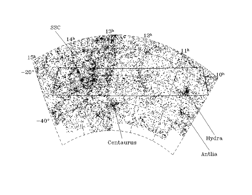
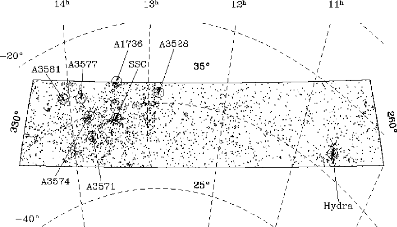
The target catalogue for the FLASH survey, containing $4613$ galaxies brighter than $b_{J}$=16.7 (corrected for Galactic extinction), was drawn from the Hydra-Centaurus Catalogue of Raychaudhury [1990, 2002]. The Hydra-Centaurus Catalogue is a photometric and morphological catalogue of $\sim$20000 galaxies down to $b_{J}$=17 in an extended region of sky in the general direction of the Great Attractor. Part of the Hydra-Centaurus Catalogue is plotted in an equal-area Aitoff projection in Figure 1, which also shows the rectangular $60\degr\times 10\degr$ region of the FLASH survey, bounded by Galactic latitude $l$=260°–330° and Galactic longitude $b$=25°–35°. The FLASH survey region is located just south of the NGP regions of the Sloan [2000] and 2dF [2001] redshift surveys: it does not overlap with either of them.

The Hydra-Centaurus Catalogue was compiled by scanning 110 UKST Southern Sky Survey plates (IIIa-J emulsion), using the Automated Photographic Measuring (APM) facility in Cambridge. For each object detected on the plate, the APM measures the position, intensity, and various shape parameters. The $(x,y)$ position of each object is converted to RA and Dec using a six-parameter transformation, with a radial correction to compensate for the projection effects of the sky onto the Schmidt plate. Absolute positions determined in this way are good to typically about $1\arcsec$.

The APM-measured magnitudes are converted to $b_{J}$ magnitudes by calibration with CCD photometry. Since Schmidt plates overlap slightly, magnitude calibration from field to field is possible using the galaxies in the overlap region which, for the Hydra-Centaurus Catalogue, averages to approximately 16 galaxies in each overlap region. From these repeat measurements, the magnitude system on each field can be matched on to a common system to better than $\sim 0^{m}.1$. It should be noted, however, that bright objects on the plates may be saturated at the centre, in which case the APM is unable to produce an accurate magnitude. Objects with magnitudes brighter than $b_{J}=14.5$ cannot therefore be used in magnitude-sensitive analyses.

All methods that attempt to distinguish between stars and galaxies using shape parameters rely on the fact that for stars the images are more centrally peaked, and described by the point-spread function, while for galaxies the images are characterised by broader profiles [1990]. This method breaks down when the images are very faint ($b_{J}\!>\!20$ on UKST J–plates, since stars and galaxies tend to look similar), or very bright ($b_{J}\!<\!15$, since the star becomes more saturated at the centre, while the wings of the stellar profile begin to approach galaxy-like proportions). The latter effect prevents completely automated star-galaxy separation (as in the APM survey, Maddox et al. 1990) for our sample.

A preliminary star-galaxy separation using the usual shape parameters like the second-order moments of each image and their areal profiles [1996, 2002] was performed on each plate with conservative separation parameters. The resulting list of galaxy candidates were then inspected by eye. A finding chart with ellipses that correspond to the shape parameters found by the APM simplifies this process, while also allowing one to inspect how well the APM is detecting all of the image (important for accurate magnitude determination). During the inspection process, galaxies were assigned broad morphological classifications as well (see Table 2). Further details can be found in Raychaudhury [2002].

In pre–1988 APM scans, due to the nature of the background subtraction algorithm and the memory allocation during image identification, most galaxies larger than $1\arcmin$ were ignored. We have assumed that all such large galaxies would be in the ESO, PGC and RC3 catalogues, from where we added all eligible galaxies found in the survey region. Galaxies added in this way are marked (see Table 2)–their positions, diameters and magnitudes would have larger uncertainties than the rest of the sample. All galaxies thus added were visually checked to prevent duplication due to mis-identification or positional errors.

About 13.5% of the galaxies in the sample belong to “merged” images, where the image parameters output by the APM refer to a combined image of the galaxy in question and other overlapping stars or galaxies (classification label $\geq$81 in Table 2. The diameters and magnitudes of these galaxies will of course be uncertain. We have visually assessed each of these objects to ensure that the galaxy in question is bright enough to be included in the sample.

The UK Schmidt plates have generous overlaps with neighbouring plates, since their centres are 5 degrees apart whereas the usable areas of these plates are 6.2 degrees square. A relative magnitude system is thus established by matching the magnitudes of galaxies in these overlap regions. CCD observations of galaxy sequences on a large fraction of of these plates are used to relate it to the $b_{J}$ magnitude system [2002]. Since total magnitudes of the calibrating galaxies are used, the quoted magnitudes refer to the total magnitude of the sample galaxies.

The galaxy magnitudes were corrected for Galactic extinction according to Burstein & Heiles [1982] reddening values based of H I column densities, using a gas-to-dust ratio of $A_{B}=4.0*E(B-V)$. The magnitude limit of $b_{J}=16.7$ was imposed after correction for extinction.

3 Observations

Most of the observations were performed with the FLAIR-II fibre spectrograph (hereafter FLAIR) system at the UK Schmidt Telescope (UKST) at Siding Spring Observatory (SSO) in Australia, over a 5-year period from mid 1991 to early 1996.

The FLAIR system [1994] was chosen as the primary observing instrument because it best matched the requirements of the FLASH survey. With $\sim$90 fibres across a Schmidt field (40 deg²), the FLAIR system is well-suited to large area, relatively bright surveys ($B\leq 18$), and is most efficient when the number density of objects is in the range 1–10 deg^-2. The FLASH survey contains $4613$ objects across 605 deg² of sky, and thus is ideally suited to an instrument like FLAIR. Although other fibre-spectrograph systems on larger telescopes have more fibres, they also have much smaller fields of view, and so are inefficient compared to FLAIR when the surface density of objects is low and the survey region covers a large area of sky.

With the FLAIR system, it is natural to tile the survey region using the the UKST Sky Survey fields, since the fibres are directly positioned onto the images of the target galaxies on Sky Survey copy plates. For each Schmidt field, a target list containing 90–100 galaxies was generated from the survey catalogue. If the field is densely populated, further target lists were created and the field re-observed. Once selected, the target galaxies were marked on UKST Sky Survey plate copies, along with at least 5 fiducial stars scattered evenly around the field, and a suitable guide star near the centre of the field.

Although the observer is assisted by a robotic system known as AutoFred [1993], the fibering process is essentially performed by hand. A small monitor allows the volunteer to see a close-up of the Schmidt plate around each target galaxy, and to mark the centre of the galaxy’s image. A ‘button’ holding a right-angle prism feeding a 100$\mu m$ (6$\aas@@fstack{\prime\prime}$7) diameter fibre is then attached to the robotic gripper arm. A carefully measured amount of bonding agent is placed on the base of the button, and the robotic arm is lowered to the plate. The fibre bundle is back-illuminated by a small lamp, which allows a computer to estimate the centroid of the fibre. Minute manual adjustments are made to the position of the gripper until the fibre centroid matches the position of the galaxy marked earlier. This process is quite quick, and results in the fibre being positioned onto the target galaxy to within the required $10\mu m$ (0$\aas@@fstack{\prime\prime}$7) accuracy. The fibre is then illuminated with UV light for 25s, which cements the fibre button onto the plate.

As many fibres as possible are placed onto target galaxies, with the intention of achieving a sampling rate close to 1-in-1. In those cases where significant over-densities existed in the field, a second or third fibre configuration for the field was observed.

As with any multi-fibre system, the finite size of the button limits how close together one can place the fibres on the plate. This can be a problem in the over-dense regions, although multiple observations of densely-populated fields, coupled with the flexibility of the FLAIR system with respect to positioning the fibres, reduce the severity of this problem. The size of the gripper limits how close to the field edge one can place a fibre, and a small $11\arcmin\times 199\arcmin$ rectangular area from the centre of the field to the bottom of the plate is obscured by the guide-star fibre bundle.

Around 6–10 fibres are reserved for observing sky. These are placed evenly across the plate on image-free patches of sky, although for improved sky subtraction it is also a good idea to place more sky fibres near densely-placed fibres. A small coherent fibre bundle, placed on a bright star close to the centre of the field, is used for coarse acquisition of the field and for guiding. Another 5 fibres, with thinner 55$\mu m$ cores, are placed on moderately bright stars scattered around the field, used as astrometric fiducials in the fine acquisition and alignment of the field.

Once fibering is complete, the plate is tensioned to obtain the correct curvature for the Schmidt telescope focal plane, the plateholder is loaded into the telescope, and the fibre bundle is connected to the spectrograph. The guide star is used to find the centre of the field, and the fiducial stars are used to acquire the correct rotation of the field. They are also used to help track the field across the sky during the night.

The survey observations used the 300B grating (300 lines/mm, blazed in the blue), giving an observable wavelength range from about 4000Å to 7000Å, and a resolution of about 5Å/pixel (FWHM$\approx$2.5Å). This setup allowed the detection of the 4000Å break down to almost zero redshift, and the detection of H$\alpha$ in emission out to redshifts of $z\sim 0.1$.

Individual exposures were typically 2000$s$ long, and up to 10 exposures of a single field could be taken in a clear half-night. (The FLAIR system could only observe one or two fields per night due to the limited number of fibre plate-holders and the long time required for manual fibre configuration.) Individual exposures were combined during the reduction process to remove cosmic rays and to improve the signal-to-noise ratio of the spectra.

4 Data Reduction

Data reduction for the spectroscopy consists of extracting each individual one-dimensional fibre spectrum from the two-dimensional data frame, calibrating the wavelength scale of the spectra, and subtracting the sky background. All these activities were performed with the flair data reduction package in iraf [1994].

Bias frames were taken each night. Where possible, sky flats were taken for fibre-throughput calculations; otherwise dome flats were used. Arc exposures for wavelength calibration were taken before and after the observations of each field. Two types of arcs were used to produce sufficient numbers (20–25) and coverage of emission lines across the wavelength range of interest: Ne for the red end and Hg-Cd for the blue. No discernible wavelength shifts were ever measured between the arc exposures taken half a night apart on either side of the survey exposures. This is due to the fact that the spectrograph in the FLAIR system is mounted on an optical bench on the floor of the dome rather than on the telescope itself, thereby avoiding flexing of the spectrograph unit as the telescope follows the target field across the sky.

The object exposures were combined to form a single object image, which was then processed by the iraf task dohydra. This task uses the combined sky-flat image to identify the position of the spectra in the object image, although it does require manual intervention at times, as the spectra on the object image are 1–3 pixels wide with only a $\sim 2$ pixel separation. The relatively even illumination across the twilight sky image ensures that the spectra are correctly traced from the red wavelengths to the blue. Third-order polynomials are quite adequate to fit the trace of the spectra, with typical rms errors being 0.1–0.2 pixels.

The combined flat-field frames were then used to calculate the relative fibre throughput, for which compensations are made in the extracted spectra. Fibre throughput tends to degrade with time as dust and grime accumulate on the prisms. As the system ages, the glue between the prism and fibre becomes more opaque and accidental kinks in the fibres take their toll. Misalignment in the mounting of the prism on the fibre buttons due to maintenance repairs or knocks in positioning, and poor seating of the fibre button the plate during configuration, also reduce a fibre’s throughput, as do telescope vignetting and the variation in transmission of a fibre from the manufacturing process.

The wavelength calibration is based on identifying 20–25 lines in the arc spectra and fitting these with third- or fourth-order polynomials to obtain the wavelength–pixel relation. Typical rms errors in the fits are about 0.1 pixels, or about 0.5Å.

The individual sky spectra are then inspected, and any spectrum contaminated by light bleeding from bright objects in neighbouring fibres is removed before the sky spectra are combined. Although potentially a serious problem, contamination from neighbouring fibres is quite rare, and tends to manifest as a modification of the spectral continuum of both objects and sky. This does not affect the position of spectral lines, but only the strength of the lines relative to the continuum; for measuring redshifts it is therefore not a particular problem except where the sky spectrum, and hence sky subtraction, is affected. There is often considerable variation in the sky spectra due to the large field of view of the Schmidt telescope, which results in the sky fibres sampling parts of the sky up to 6° apart. Most of the variations are in the strengths of the strong O i emission features at 5577Å, 6300Å and 6363Å, while the continuum tends to remain unaffected. This results in good continuum subtraction, but poor subtraction of the strongly-varying sky lines, which can lead to difficulties in identifying spectral features near these lines.

5 Redshifts

5.1 Redshift Measurements

Once the spectra have been extracted, sky-subtracted, and wavelength-calibrated, radial velocity (redshift) measurements can be made. The CCD on the FLAIR system prior to 1995 had a rather poor response in the blue, making it difficult to identify the Ca H and K lines and the G band. While the new thinned CCD is twice as responsive in the blue, these lines can still be quite difficult to detect. Other lines used in the process of measuring the redshift were H$\beta$ at 4861Å, [O iii] at 4959Å and 5007Å, the Mg b triplet around 5175Å, the Fe features at 5207Å and 5270Å, Na D at 5892Å, H$\alpha$ at 6563Å, N ii at 6584Å, and the S ii doublet at 6716Å and 6731Å.

Using the iraf task rvidlines, gaussians were fitted to each identified feature in the spectrum to determine the position of the line and hence its shift. The line shifts are then averaged to produce a final radial velocity measurement, while the standard deviation of the line shifts gives the internal radial velocity error. These errors were typically less than 100 km s^-1 (see below).

Additional redshifts for the FLASH survey catalogue were obtained from the literature via the NASA/IPAC Extragalactic Database (NED) and the ZCAT catalogue [1999]; 901 redshifts were obtained from ZCAT, and 354 were obtained from NED.

The final estimate of the galaxy’s redshift is the variance-weighted mean of the measured redshifts from FLAIR (including repeat measurements for some objects) and the literature. A further, subjective, weighting was applied to the literature-derived redshifts, reflecting our degree of belief in the estimated redshift errors in the literature—in short, NED and ZCAT redshifts were given half the weight of the FLAIR redshifts.

5.2 Internal and External Errors

One can check the precision of the FLAIR redshifts by comparing the multiple radial velocity measurements for those galaxies that have repeat observations. The redshift differences for the 164 galaxies with multiple redshift measurements are plotted in the top panel of Figure 2. The mean offset is $-$0.4 km s^-1; the standard deviation in the difference is 134 km s^-1, indicating an rms error in the redshifts of 95 km s^-1 (assuming equipartition of errors).

Figure 2: Comparing redshifts measured on the FLAIR system with (top) repeat FLAIR measurements, and (bottom) literature redshifts. Solid curves are gaussians with the median and standard deviation about the median of each distribution: $-$0.4 km s^-1 and 134 km s^-1 for the top panel, and $-$22 km s^-1 and 146 km s^-1 for the bottom panel.

Although we have been careful in estimating the redshift errors, there may be effects (systematic or otherwise) that have not been accounted for. To detect such effects and determine the reliability of the estimated errors, one can compare the variance-weighted estimated errors, $\overline{\sigma}$, with the rms errors, $\sigma_{\rm RMS}$, for the 164 objects with repeat measurements.

The top panel of Figure 3 shows both the differential (histogram) and cumulative (stepped line) distributions of the ratio $\sigma_{\rm RMS}/\overline{\sigma}$ for all the objects with multiple FLAIR redshift measurements. The corresponding smooth curves are the predicted differential and cumulative distribution functions for this quantity assuming the estimated errors are correct and the error distributions are gaussian [1999]. The top panel of Figure 3 shows that the errors are under-estimated, since, from the cumulative distributions, it is evident that the ratio of the rms to estimated errors is always greater than expected.

This under-estimation of the errors in the FLAIR redshifts results from the way the errors were estimated from the spectra. The rvidlines algorithm finds the rms error of the gaussian fits to the individual line profiles, and so produces an internal error; however, external errors (such as wavelength calibration errors, mis-alignment of the fibre and the centre of the galaxy, or miscellaneous instrumental offsets) can also contribute to the overall error in the measured redshift.

Figure 3: Comparison of estimated errors to rms errors from repeat measurements. The top panel shows the comparison using the raw estimated errors; the bottom panel shows the comparison using the corrected estimated errors.

We find empirically that adding 40 km s^-1 in quadrature to the estimated errors optimises the match between the estimated errors and the rms errors (maximising the probability that the predicted and observed distributions of $\sigma_{\rm RMS}/\overline{\sigma}$ are the same in a Kolmogorov-Smirnov test). The resulting distribution of $\sigma_{\rm RMS}/\overline{\sigma}$ is shown in the lower panel of Figure 3, where the improved agreement is quite evident. The median rms error (re-calculated allowing for this correction) is 103 km s^-1. This is consistent with the results of Watson [1991], who showed that the FLAIR system could reproduce redshifts to better than 150 km s^-1 for $b_{J}\!\sim\!17$ galaxies.

We can also obtain an external estimate of the errors in the FLAIR redshifts using the 393 objects with both FLAIR and literature redshifts. The lower panel of Figure 2 shows the distribution of the difference in redshifts between FLAIR and literature measurements, after re-computing the variance-weighted FLAIR redshifts using the corrected estimated errors. The mean offset is $-$22 km s^-1 with a standard deviation of 146 km s^-1, which, with equipartition of errors, implies an rms redshift error of 103 km s^-1, in excellent agreement with the corrected estimated errors.

6 Redshift Completeness and Bias

Table 1: Statistical properties of the Schmidt fields in the FLASH survey region.

(1)	(2)	(3)	(4)	(5)	(6)
Field	Field Center		$\rm N_{gal}$	$\rm N_{cz}$	Completeness
	RA	Dec
322	12 34	–40 00	1	1	1.00
323	13 00	–40 00	3	1	0.33
377	11 12	–35 00	26	4	0.15
378	11 36	–35 00	90	50	0.56
379	12 00	–35 00	90	61	0.68
380	12 24	–35 00	118	90	0.76
381	12 48	–35 00	150	97	0.65
382	13 12	–35 00	220	173	0.79
383	13 36	–35 00	253	215	0.85
384	14 00	–35 00	175	133	0.76
385	14 24	–35 00	40	9	0.22
436	10 21	–30 00	9	9	1.00
437	10 44	–30 00	133	68	0.51
438	11 07	–30 00	97	62	0.64
439	11 30	–30 00	79	66	0.84
440	11 53	–30 00	243	127	0.52
441	12 16	–30 00	107	76	0.71
442	12 39	–30 00	94	70	0.74
443	13 02	–30 00	341	280	0.82
444	13 25	–30 00	437	347	0.79
445	13 48	–30 00	328	234	0.71
446	14 11	–30 00	203	120	0.59
447	14 34	–30 00	225	109	0.48
499	09 54	–25 00	2	1	0.50
500	10 16	–25 00	75	59	0.79
501	10 38	–25 00	185	158	0.85
502	11 00	–25 00	85	47	0.55
503	11 22	–25 00	61	37	0.61
504	11 44	–25 00	49	30	0.61
505	12 06	–25 00	28	5	0.18
506	12 28	–25 00	1	1	1.00
508	13 12	–25 00	14	11	0.79
509	13 34	–25 00	85	42	0.49
510	13 56	–25 00	172	109	0.63
511	14 18	–25 00	141	83	0.59
512	14 40	–25 00	15	5	0.33
567	10 09	–20 00	49	36	0.73
568	10 30	–20 00	106	84	0.79
569	10 51	–20 00	52	27	0.52
570	11 12	–20 00	5	0	0.00
638	10 20	–15 00	19	2	0.11
639	10 40	–15 00	7	2	0.29

(1) Schmidt field ID; (2) Field centre right ascension (B1950); (3) Field centre declination (B1950); (4) Number of galaxies in the field belonging to our sample; (5) Number of galaxies with redshifts; (6) Field completeness (percentage of redshifts measured).

Incompleteness within a survey can occur in several ways, and for many reasons. If an incompleteness is systematic with respect to an observable quantity, it can seriously affect any analysis performed on the survey data if it is uncorrected. Incompleteness can be corrected for when it relates to a quantity that is known for every object in the input catalogue (e.g. magnitude or morphological type), but not if it is due to a quantity that is being measured (e.g. redshift). To correct for an incompleteness, one may simply assign an appropriate weight to each galaxy, although for some analyses, a simple weighting strategy will not work, and the incompleteness must be factored into the analysis directly.

The overall redshift completeness of the FLASH survey is 0.64, with redshifts for $3141$ of the $4613$ galaxies in the catalogue. We now consider the dependence of this completeness on observing conditions (field), on apparent magnitude, and on redshift itself.

6.1 Field Completeness

Because we observe galaxies with FLAIR one Schmidt plate at a time, there is a field-to-field variation in completeness that depends on the quality of the observing conditions for each field. Figure 6 shows the Schmidt fields that tile the FLASH survey region, with the field number shown in the top left and the field redshift completeness centred on each field.

The redshift completeness across the survey region is reasonably uniform given the variation in galaxy number density across the sky in the region (see Figure 1). The median completeness over all 42 fields is 0.63. The reason this figure is lower than the overall completeness is that the lower-completeness fields tend to be near the edge of the survey region, where the number of galaxies within the survey is too small to be able to use the FLAIR system efficiently, so that galaxy redshifts in these fields are predominantly from the literature.

Figure 4: Redshift completeness as a function of (corrected) apparent magnitude for all galaxies in the FLASH survey. The dashed line is the fit used in applying the magnitude-dependent completeness correction of the data: $f(m)=-0.96+0.43m-0.020m^{2}$ for apparent magnitudes $m>14.2$, and $f(m)=1$ otherwise.

Figure 5: Redshift completeness as a function of (corrected) apparent magnitude for early and late morphological types in the FLASH survey. The dashed line is the fit used in applying the magnitude-dependent completeness correction of the data. For early types: $f(m)=0.00088+0.32m-0.018m^{2}$ for $m>14.2$, unity otherwise. For late types: $f(m)=0.21+0.27m-0.015m^{2}$, for $m>14.2$, unity otherwise.

Figure 6: Variation in redshift completeness from field to field in the FLASH survey.

Table 1 lists the statistics of each Schmidt field in the survey region. For each field the table contains the following information: field ID number, R.A. and Dec. of the field centre (B1950), number of target galaxies, number of redshifts obtained, and field completeness.

6.2 Apparent Magnitude Completeness

The signal-to-noise ratio in the observed spectra decreases as the target objects’ apparent magnitudes become fainter. This results in a decreasing redshift completeness at fainter apparent magnitudes which, if not corrected for, will result in an incorrect selection function and skew the results obtained from magnitude-dependent analyses (e.g. the luminosity function).

The completeness as a function of apparent magnitude for the whole survey sample is shown in Figure 4, and for early and late morphological types separately in Figure 5. Both figures show a rapid drop in completeness beyond $b_{J}$=15, with approximately 50 per cent completeness at the survey’s magnitude limit. Also shown in the figures are the best-fit polynomial functions approximating the completeness variation over the magnitude range (dashed lines). These functions are used in applying the magnitude-dependent completeness corrections in later papers.

6.3 Redshift Bias

In early May and mid April 1994, 34 redshifts were obtained with the Double Beam Spectrograph (DBS) on the ANU 2.3m telescope at SSO. The target galaxies were a selection of objects observed with FLAIR for which redshifts were not obtained. The purpose of these further observations was to explore the possibility that the FLASH survey might be biased against obtaining redshifts for some subset of objects in the target catalogue on the basis of their spectral type or redshift.

The top panel of Figure 7 shows the number–magnitude distribution of galaxies for which redshifts were obtained with FLAIR or the ANU 2.3m in the same fields. Clearly the objects that failed to have a redshift measured with FLAIR (the ANU 2.3m sample) are at the faint end, with typical apparent magnitudes fainter than $m_{b_{J}}$=15.5, consistent with Figure 4.

The bottom panel of Figure 7 shows the number–redshift distribution of the FLAIR and 2.3m samples, along with the cumulative distributions from each sample. The number–redshift distributions for the FLAIR sample and 2.3m sample appear quite consistent. We use the Kolmogorov-Smirnov statistic to quantitatively test the hypothesis that the galaxies with and without FLAIR redshifts come from the same underlying redshift population. We find that the two redshift distributions are consistent at the 74 per cent confidence level.

We can conclude, therefore, that the galaxies observed with FLAIR for which no redshifts were obtained have the same redshift distribution as those for which we obtained FLAIR redshifts. The only redshift bias in the FLASH survey is that due to magnitude-dependent incompleteness, and can therefore be corrected in a straightforward manner.

Figure 7: Comparison of redshift distributions for objects with and without FLAIR redshift measurements. Redshifts for the latter were obtained with the ANU 2.3m telescope. The top panel shows the magnitude distributions of the two samples. The bottom panel shows the differential and cumulative redshift distributions.

7 The FLASH Survey Catalogue

The FLASH survey includes a total of $3141$ redshifts over 605 deg² of sky. An example subset of the FLASH survey catalogue is presented in Table 2. The full survey catalogue is available from NASA’s Astrophysical Data Centre (ADC; http://adc.gsfc.nasa.gov/adc.html) and the Centre de Données astronomiques de Strasbourg (CDS; http://cdsweb.u-strasbg.fr/). Each entry in the table contains: the Schmidt field the galaxy was observed in, the galaxy’s R.A. and Dec. (B1950), the magnitude ($b_{J}$), major axis diameter (arcmin), morphological type, heliocentric radial velocity and error (km s^-1), and source reference for the radial velocity (FLAIR, 2.3m, NED, ZCAT). The magnitudes were extinction-corrected according to Burstein & Heiles [1982], using $A_{B}=4.0*E(B-V)$.

Figure 8 displays those galaxies in the FLASH survey catalogue with measured redshifts in an equal-area Aitoff projection. Clusters and filamentary structures are clearly evident across the survey region: the Shapley Supercluster dominates the survey region near $(l,b)$=(312°, 31°); the Hydra cluster of galaxies is clearly visible at the lower right of the plot; a number of other prominent Abell clusters are indicated on the figure. The flattened structure spanning the survey region north-south at about $13^{h}$ (see also Figure 1) is the Supergalactic Plane, the projection onto the sky of the Local Supercluster.

Figure 8: The distribution of the FLASH survey galaxies with measured redshifts on the sky, shown in an equal-area Aitoff projection. Some of the more prominent clusters within the survey region are indicated. The “SSC” refers to the four clusters in the core of the Shapley Supercluster, consisting of the A3558, SC1327-312, SC1329-313 and A3562 clusters.

Table 2: The FLASH survey catalogue – example data. The full survey catalogue will be available from NASA’s Astrophysical Data Centre (ADC; http://adc.gsfc.nasa.gov/adc.html) and the Centre de Données astronomiques de Strasbourg (CDS; http://cdsweb.u-strasbg.fr/).

(1)	(2)	(3)	(4)	(5)	(6)	(7)	(8)	(9)	(10)	(11)
Field	RA	Dec	$\ell$	b	$b_{J}$	$D$	$T$	$cz$	$\sigma$	cz
	(B1950)		(°)	(°)	(mag)	(′)		(km s-1)		src
499	10 03 24.84	-23 38 21.8	261.0	25.2	16.6	0.5	1	0	0	-
499P	10 03 36.00	-22 48 48.0	260.4	25.8	14.5	1.1	2	3829	39	F
567	10 07 22.57	-22 02 43.3	260.6	27.0	16.7	0.6	3	14005	58	F
500P	10 07 43.00	-24 04 59.9	262.1	25.5	14.6	1.2	3	9565	27	N
567	10 07 59.20	-21 10 31.3	260.1	27.7	16.7	0.3	4	16740	45	F
500	10 08 13.14	-23 43 56.7	262.0	25.8	15.8	0.5	4	9699	112	F
500	10 08 31.25	-22 54 40.5	261.5	26.5	15.8	1.0	3	9689	190	F
567	10 08 40.86	-22 26 04.8	261.1	26.9	15.3	0.8	1	3665	111	F
567	10 08 46.35	-21 17 05.3	260.3	27.8	15.4	0.7	3	9323	10	F,Z
567	10 09 07.76	-21 03 01.1	260.2	28.0	16.0	0.4	3	9110	70	F
567	10 09 14.69	-20 54 37.0	260.2	28.1	16.3	0.7	84	0	0	-
567P	10 09 15.54	-21 00 23.6	260.2	28.1	14.2	0.7	3	8972	10	N,Z
567	10 09 17.71	-21 07 11.5	260.3	28.0	15.9	0.5	4	9274	54	F
500	10 10 43.88	-23 12 17.9	262.1	26.6	16.5	0.5	3	15593	70	F
500P	10 11 13.12	-22 30 35.3	261.7	27.2	15.3	0.9	3	3617	32	F
500	10 11 15.32	-23 15 01.4	262.2	26.6	16.4	0.4	3	23911	75	F
500P	10 11 40.01	-25 23 30.0	263.8	25.0	16.0	1.2	3	0	0	-
567P	10 11 42.00	-21 43 42.0	261.2	27.9	14.1	2.2	3	3615	6	F,N
567	10 12 00.73	-20 08 42.3	260.2	29.1	15.7	0.9	83	3465	109	F
500	10 12 08.97	-22 48 04.9	262.1	27.1	16.0	0.5	2	5094	35	F
567	10 12 18.36	-20 45 42.7	260.7	28.7	15.9	0.8	3	0	0	-
567P	10 12 21.19	-20 33 40.8	260.5	28.9	15.2	1.2	3	3595	51	F
567	10 12 30.68	-20 42 55.5	260.7	28.8	16.3	0.8	3	0	0	-
567	10 12 31.26	-20 30 16.2	260.5	28.9	16.2	0.4	4	0	0	-
500	10 12 32.51	-22 48 00.2	262.2	27.2	15.2	1.0	1	3679	25	F,N
500	10 12 45.93	-24 57 13.5	263.7	25.5	16.6	0.5	3	11740	108	F
567	10 13 01.52	-22 18 41.4	261.9	27.6	15.8	0.6	83	0	0	-
567	10 13 10.01	-20 20 04.4	260.5	29.2	15.7	0.6	1	0	0	-
567	10 13 12.13	-19 45 59.1	260.1	29.6	16.2	0.5	82	14423	60	F
567P	10 13 14.19	-20 23 52.8	260.6	29.1	13.6	1.8	2	3565	35	F,N
567	10 13 21.67	-20 02 46.1	260.4	29.4	14.0	1.6	3	3653	22	F,N
567	10 13 25.19	-21 29 12.4	261.4	28.3	15.4	0.9	83	0	0	F
567	10 13 30.68	-21 24 57.5	261.4	28.4	15.2	0.7	4	3547	54	F
567	10 13 33.61	-19 47 28.4	260.2	29.6	16.5	0.4	73	16413	42	F
567	10 13 38.65	-21 26 19.1	261.4	28.4	16.7	0.6	4	0	0	-
567	10 13 51.10	-20 20 50.8	260.7	29.3	16.5	0.4	4	12964	75	F
567	10 13 58.29	-19 56 22.6	260.4	29.6	15.7	0.8	2	0	0	-
567	10 14 07.76	-19 37 27.8	260.2	29.9	15.8	0.7	73	14925	90	F
500	10 14 20.22	-25 14 21.3	264.2	25.5	16.7	0.4	2	11894	64	F
567	10 14 27.34	-20 23 09.8	260.8	29.3	15.3	0.8	3	7046	80	F
500	10 14 30.21	-25 01 06.6	264.1	25.7	15.7	0.5	3	12042	110	F
567	10 14 32.05	-21 58 48.5	262.0	28.1	15.4	0.7	81	3932	40	F
500	10 14 37.62	-24 55 51.0	264.1	25.8	15.8	0.6	2	12627	75	F
567	10 14 50.66	-20 48 59.7	261.2	29.0	15.3	0.7	2	3478	31	F
500	10 15 18.20	-24 16 44.5	263.8	26.4	16.4	0.6	1	12289	108	F
500	10 15 20.37	-26 02 02.0	265.0	25.0	16.3	0.4	81	0	0	-
500	10 15 33.43	-24 18 39.8	263.8	26.4	16.2	1.0	3	12725	108	F
567	10 15 56.20	-22 09 48.6	262.4	28.2	15.3	0.9	3	3975	42	F

(1) The Schmidt field (“P” indicates that the position was taken from the PGC or RC3 catalogue); (2) The galaxy’s right ascension (B1950); (3) The galaxy’s declination (B1950); (4) Galactic longitude; (5) Galactic latitude; (6) $b_{J}$ magnitude; (7) Major axis diameter (arcmin); (8) Morphological type flag [1: Elliptical, 2: S0, 72: SB0, 3 : Spiral, 73: Barred Spiral, 4 : Late-type Irregular, 5 : Unknown, 81: Star + Elliptical, 82: Star + S0, 83: Star + Spiral, 84: Star + Irregular, 91: Elliptical + Elliptical, 92: Elliptical + S0, 93: Elliptical + Spiral, 94: Elliptical + Irregular, 96: S0 + Spiral, 97: Spiral + Spiral, 98: S0 + Irregular, 99: Spiral + Irregular], (9) Heliocentric redshift (km s^-1); (10) Error in redshift (km s^-1); (11) Source of redshift: F (FLAIR), T (ANU 2.3m Telescope), N (NED), Z (ZCAT, December 2000 version).

8 Discussion

The redshift distribution of the FLASH survey is shown in Figure 9. It extends out to about 30000 km s^-1 and has a median depth of about 10000 km s^-1. The APM-Stromlo [1992] and Durham/UKST [1998] redshift surveys cover factors of 6 and 2 times more sky respectively to a similar depth. However both these surveys use sparse-sampling strategies (1-in-20 and 1-in-3 respectively), which allow greater sky coverage at the expense of reducing the resolution of the large-scale structure. The FLASH survey, with a sampling rate of about 2-in-3, maps a larger number of galaxies in a smaller volume, thereby sampling the large-scale structure at a higher resolution and allowing a finer probe of the large-scale structure in the direction of the Shapley Supercluster and Hydra cluster, and better determining the effects of these structures upon the Local Group motion.

Figure 9 also shows the redshift distribution expected for a homogeneous universe with the same luminosity function parameters (as derived in a subsequent paper in this series) and selection function as the FLASH survey. In comparison to this homogeneous redshift distribution, the most outstanding features in the observed redshift distribution are the strong peaks due to the many foreground clusters at $\sim$4000 km s^-1 (including the Hydra cluster) and the Shapley Supercluster at $\sim$15000 km s^-1.

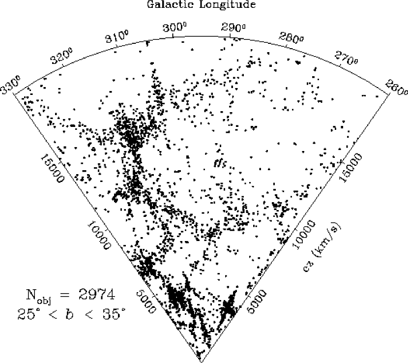
These structures and others are clearly visible in the wedge plot shown in Figure 10. In this figure, the Shapley Supercluster is the large ‘Finger-of-God’ at $l\approx 310\degr$ and $cz\approx 14000$ km s^-1, while the Hydra cluster is the sharply defined ‘Finger-of-God’ at $l\approx 270\degr$ and $cz\approx 4000$ km s^-1. There are many other clusters in the survey region, evidenced by the tell-tale ‘Fingers-of-God’ in Figure 10, most of which are Abell clusters in the direction of the Shapley Supercluster (cf. Figure 8). Along with the clusters, a number of wall-like structures can be seen, particularly in the vicinity of the Shapley Supercluster, where they form a structure similar to the famous ‘stick-man’ structure associated with the Coma cluster, that was found in the CfA redshift survey [1986].

Since the FLASH survey has morphological information, it is possible to examine the properties of each morphological type separately. We choose to divide the sample into two broad morphological types—early (E and S0) and late (Sp and Irr)—even though the type information we possess is more detailed. The reason for doing so is partly to minimize the effects of classification errors, but mainly so that there are enough objects in each grouping to allow meaningful comparisons.

Figure 9: The redshift distribution for all the galaxies in the FLASH survey with measured redshifts. The dashed line is the distribution expected from a homogeneous universe with the same luminosity function parameters and selection function as the FLASH survey.

Figure 10: Redshift wedge plot of all the galaxies in the FLASH survey, including those with unknown morphologies.

The redshift wedge plots of the early and late galaxy types are shown in Figures 11 and 12 respectively. The FLASH survey contains redshifts for $1272$ early-type galaxies, and $1802$ late-types. Although similar, the distributions of early and late types show some interesting differences. Figure 11 shows that the early-type galaxies are found predominantly within cluster cores, and less frequently within wall-like structures. The late-type galaxies are found in both clusters and wall-like structures, as shown in Figure 12, and thus can be considered as more representative tracers of the large-scale structure. A good example of this is the bridge of galaxies between $10000\leq cz\leq 15000$ km s^-1along $l=290\degr$, which is almost entirely populated with late-type galaxies, and is not visible in Figure 11.

9 Conclusion

The FLASH survey catalogue contains $4613$ galaxies brighter than $b_{J}$=16.7 within a $60\degr\times 10\degr$ region bounded by Galactic latitude $l$=260°–330° and Galactic longitude $b$=25°–35°. The galaxies are drawn from the the Hydra-Centaurus Catalogue of Raychaudhury [1990, 2002]. The FLASH survey region is richly structured, and includes the Shapley Supercluster and Hydra cluster, as well as many other Abell clusters, and the Supergalactic Plane.

The FLAIR-II fibre spectrograph at the UKST was used to obtain redshifts accurate to $\sim$100 km s^-1 for 1896 galaxies. A further 1245 redshifts were obtained from the NED and ZCAT catalogues, bringing the total number of galaxies with redshifts in the survey to $3141$ . The overall redshift completeness of the sample is 68 per cent. Although the completeness varies with apparent magnitude, dropping almost to 50 per cent at the faint survey limit, follow-up observations show that there is no explicit redshift bias. This magnitude-dependent incompleteness can therefore be corrected in a straightforward manner.

Figure 11: Redshift wedge plot for the early morphological types in the FLASH survey.

Figure 12: Redshift wedge plot for the late morphological types in the FLASH survey.

By selection, the FLASH survey region is not a fair sample of the universe. The redshift wedge plot for the whole survey region (Figure 10) reveals a remarkable amount of structure. The dominant structures are galaxy clusters, shown as ‘Fingers-of-God’ in the wedge plot, with the largest structure being the Shapley Supercluster. Walls and filaments connect the various clusters, forming in the vicinity of the Shapley Supercluster a structure similar to the ‘stick-man’ structure observed around the Coma cluster in the CfA survey, but on a much larger scale.

Different structures can be seen in the wedge plots for the early and late morphological types in the FLASH survey. The most representative tracer of large-scale structure are the late-type galaxies, which are associated with both the clusters and the wall-like structures. The early-type galaxies are less frequently associated with the wall-like structures, tending instead to be found predominantly in the cores of rich clusters.

Future papers in this series will examine the galaxy luminosity and correlation functions, with particular attention to the variations with morphological type, and reconstruct the peculiar velocity field in this volume of space in order to determine the contribution of the observed structures to the peculiar motion of the Local Group.

References

- [2000] Bardelli, S., Zucca, E., Zamorani, G., Moscardini, L., Scaramella, R., MNRAS, 2000, 312, 540
- [1993] Bedding, T., Gray, P. M., Watson, F., 1993, ASP Conf. Ser. 37: Fiber Optics in Astronomy II, p. 181
- [1982] Burstein, D., Heiles, C., 1982, AJ, 87, 1165
- [1990] Burstein, D., 1990, Rep. Prog. Phys. 53, 421
- [1999] Colless, M., Burstein, D., Davies, R. L., McMahan, R. K., Saglia, R. P., Wegner, G., MNRAS, 1999, 303, 813
- [2001] Colless, M., et al., MNRAS, 2001, submitted
- [1994] Drinkwater, M., Holman, B., FLAIR Data Reduction with IRAF, Anglo-Australian Observatory
- [1999] Drinkwater, M. J., Proust, D., Parker, Q. A., Quintana, H., Slezak, E., PASA, 1999, 16, 113
- [1997] Ettori, S., Fabian, A. C., & White, D. A. 1997, MNRAS, 289, 787
- [1991] Fabian, A. C., MNRAS, 1991, 253, 29
- [1999] Huchra, J. P., The Center for Astrophysics Redshift Catalogue, 2000, http://cfa-www.harvard.edu/huchra
- [1993] Kogut, A., Lineweaver, C., Smoot, G. F., Bennett, C. L., Banday, A., Boggess, N. W., Cheng, E. S., de Amici, G., Fixsen, D. J., Hinshaw, G., Jackson, P. D., Janssen, M., Keegstra, P., Loewenstein, K., Lubin, P., Mather, J. C., Tenorio, L., Weiss, R., Wilkinson, D. T., Wright, E. L., 1993, ApJ, 419, 1
- [1986] de Lapparent, V., Geller, M. J., Huchra, J. P., 1986, ApJ, 302, L1
- [1992] Loveday, J., Peterson, B. A., Efstathiou, G., Maddox, S. J., 1992, ApJ, 390, 338
- [1996] Loveday, J. 1996, MNRAS, 278, 1025
- [1988] Lynden-Bell, D., Faber, S. M., Burstein, D., Davies, R. L., Dressler, A., Terlevich, R. J., Wegner, G., 1988, ApJ, 326, 19
- [1990] Maddox, S. J., Efstathiou, G., Sutherland, W. J., Loveday, J., MNRAS, 243, 692
- [1987] Melnick, J., Moles, M., RMxAA, 1987, 14, 72
- [1994] Parker, Q. A., Watson, F. G. 1994, IAU Symp. 161: Astronomy from Wide-Field Imaging, 161, 85
- [1995] Quintana, H., Ramirez, A., Melnick, J., Raychaudhury, S., Slezak, E., AJ, 1995, 110, 463
- [1998] Ratcliffe, A., Shanks, T., Parker, Q. A., Broadbent, A., Watson, F. G., Oates, A. P., Collins, C. A., Fong, R., 1998, MNRAS, 300, 417
- [1989] Raychaudhury, S., 1989, Nat, 342, 251
- [1990] Raychaudhury, S., 1990, PhD thesis, University of Cambridge
- [2002] Raychaudhury, S., 2002, in preparation
- [1991] Raychaudhury, S., Fabian, A. C., Edge, A. C., Jones, C., Forman, W., MNRAS, 1991, 248, 101
- [1991] Watson, F. G., Oates, A. P., Shanks, T., Hale-Sutton, D., 1991, MNRAS, 253, 222
- [2000] York, D. G. et al. 2000, AJ, 120, 1579