Inflaton potential reconstruction in the braneworld scenario

Abstract

We consider inflaton potential reconstruction in the context of the simplest braneworld scenario, where both the Friedmann equation and the form of scalar and tensor perturbations are modified at high energies. We derive the reconstruction equations, and analyze them analytically in the high-energy limit and numerically for the general case. As previously shown by Huey and Lidsey, the consistency equation between scalar and tensor perturbations is unchanged in the braneworld scenario. We show that this leads to a perfect degeneracy in reconstruction, whereby a different viable potential can be obtained for any value of the brane tension $\lambda$. Accordingly, the initial perturbations alone cannot be used to distinguish the braneworld scenario from the usual Einstein gravity case.

I Introduction

Upcoming observations, particularly of cosmic microwave anisotropies, have the prospect of placing the first serious constraints on models for the origin of structure, amongst which inflation is currently the leading candidate (see Ref. LL for an extensive review). Provided the inflationary paradigm remains successful, an ultimate goal is the ‘reconstruction’ of the inflaton potential from observable quantities CKLL ; LLKCBA . Attention has primarily been focussed on the case of single-field slow-roll inflation, as it provides a class of simple models which can be considered within a common framework.

In order to have a robust interpretation of upcoming observations, such as those of cosmic microwave background anisotropies by the MAP and Planck satellites, it is imperative to develop an understanding of how the reconstruction process may be affected by degeneracies, whereby different cosmological models give rise to identical or near-identical observational predictions. Degeneracies have been considered in some depth as far as the usual cosmological parameters are concerned, the most important one being connected to the angular diameter distance to the last-scattering surface. As far as the initial perturbations are concerned, the most significant degeneracy discussed thus far is an approximate degeneracy between a tensor contribution to the anisotropies and the effect of early reionization, which though approximate requires accurate polarization measurements to be significantly broken.

A different possible degeneracy concerns the inflationary models themselves, and whether there might be different models giving rise to the same initial spectra of scalar and tensor perturbations. For single-field slow-roll models, there is a unique correspondence between the tensor spectrum and the inflationary potential, whereas if only the scalar perturbations can be observed there remains a one-parameter perfect degeneracy leading to a family of possible potentials CKLL . In this paper, we consider whether there might be additional degeneracies associated with the possibility that the physics of inflation might go beyond Einstein gravity with a single scalar field. Specifically, we consider the simplest incarnation of the braneworld scenario, in which at high energies both the classical background evolution and the form of the perturbations are modified. We will show that this leads to a perfect degeneracy even if both tensor and scalar perturbations are measured. This shows that the initial perturbations alone cannot be used to distinguish the braneworld scenario from the usual Einstein gravity one.

II Basic formulae

We restrict ourselves throughout to the simplest braneworld scenario bin ; shiro , based on the type-II Randall–Sundrum model RSII , where the Friedmann equation receives an additional term quadratic in the density. We use the slow-roll approximation, as formulated by Maartens et al. MWBH . Using the definitions of Ref. LLKCBA , the spectra of scalar MWBH and tensor LMW ; HL spectra are given by

$$A_{{\rm S}}^{2} = \frac{4}{25}\,\frac{H^{2}}{\dot{\phi}^{2}}\,\left(\frac{H}{2\pi}\right)^{2}\simeq\frac{512\pi}{75M_{4}^{6}}\,\frac{V^{3}}{V^{\prime 2}}\,\left(1+\frac{V}{2\lambda}\right)^{3}\,;$$ (1)

$$A_{{\rm T}}^{2} = \frac{4}{25\pi}\,\frac{H^{2}}{M_{4}^{2}}\,F^{2}(H/\mu)\,,$$ (2)

where

$$F(x) = \left[\sqrt{1+x^{2}}-x^{2}\ln\left(\frac{1}{x}+\sqrt{1+\frac{1}{x^{2}}}\right)\right]^{-1/2}\,,$$ (3)

$$= \left[\sqrt{1+x^{2}}-x^{2}\sinh^{-1}\frac{1}{x}\right]^{-1/2}\,,$$

and the slow-roll approximation has been used to obtain expressions in terms of the inflaton potential $V(\phi)$. Here $M_{4}$ is the four-dimensional Planck mass, and $\lambda$ is the brane tension. The mass scale $\mu$ is given by

$$\mu=\sqrt{\frac{4\pi}{3}}\,\sqrt{\lambda}\,\frac{1}{M_{4}}\,,$$ (4)

prime indicates derivative with respect to the scalar field $\phi$, and dot a derivative with respect to time.

The Hubble parameter $H$ is related to the energy density $\rho$ by

$$H^{2}=\frac{8\pi}{3M_{4}^{2}}\,\rho\,\left(1+\frac{\rho}{2\lambda}\right)\simeq\frac{8\pi}{3M_{4}^{2}}\,V\,\left(1+\frac{V}{2\lambda}\right)\,,$$ (5)

which reduces to the usual Friedmann equation for $\rho\ll\lambda$, the scalar field obeys the usual slow-roll equation

$$3H\dot{\phi}\simeq-V^{\prime}\,,$$ (6)

and the amount of expansion, in terms of $e$-foldings, is given by

$$\frac{dN}{d\phi}=\frac{H}{\dot{\phi}}$$ (7)

The expressions for the spectra are, as always, to be evaluated at Hubble radius crossing $k=aH$, and the spectral indices of the scalars and tensors are defined as usual by

$$n-1\equiv\frac{d\ln A_{{\rm S}}^{2}}{d\ln k}\quad;\quad n_{{\rm T}}\equiv\frac{d\ln A_{{\rm T}}^{2}}{d\ln k}\,.$$ (8)

If one defines slow-roll parameters, generalizing the usual ones, by MWBH

$$\epsilon_{{\rm B}} \equiv \frac{M_{4}^{2}}{16\pi}\,\left(\frac{V^{\prime}}{V}\right)^{2}\;\frac{1+V/\lambda}{\left(1+V/2\lambda\right)^{2}}\,;$$ (9)

$$\eta_{{\rm B}} \equiv \frac{M_{4}^{2}}{8\pi}\,\frac{V^{\prime\prime}}{V}\;\frac{1}{1+V/2\lambda}\,,$$ (10)

then the scalar spectral index, in the slow-roll approximation, obeys the usual equation

$$n-1\simeq-6\epsilon_{{\rm B}}+2\eta_{{\rm B}}\,.$$ (11)

The tensor index obeys a more complicated equation, but remarkably it still obeys the usual consistency equation HL

$$R\equiv\frac{A_{{\rm T}}^{2}}{A_{{\rm S}}^{2}}=-\frac{1}{2}n_{{\rm T}}\,.$$ (12)

This result is maintained because the normalization of the tensor mode function requires $F(x)$ to obey a particular differential equation. This tells us that the relation between scalar and tensor perturbations is unchanged in the braneworld scenario. In particular, this equation can be viewed as an expression giving the scalar spectrum corresponding to a given tensor spectrum, namely

$$A_{{\rm S}}^{2}=-2\frac{A_{{\rm T}}^{2}}{n_{{\rm T}}}=-\frac{A_{{\rm T}}^{3}}{dA_{{\rm T}}/d\ln k}\,.$$ (13)

Hence in the braneworld scenario, as in Einstein gravity, the scalars carry no additional information about the potential if the tensors are known. This invariance of the consistency relation under a change in gravitational physics is unexpected, since in most variations of standard inflation, e.g. warm inflation TB00 , this relation is substantially different.

II.1 Low-energy limit

Provided $\rho\ll\lambda$, the equations all reduce to the usual Einstein gravity ones and the normal reconstruction equations apply. In particular, if one is able to observe the tensor spectrum, it gives a unique potential (under the single-field assumption), and if the scalars can additionally be measured they obey consistency relations. If only the scalars can be measured, a unique potential cannot be obtained and there is a one-parameter family of possible models. Measurement of the tensors at a single scale is sufficient to remove this degeneracy.

II.2 High-energy limit

Before proceeding to the general case, it is instructive to analyze the high-energy limit. The key expressions are

$$A_{{\rm S}}^{2} \simeq \frac{64\pi}{75M_{4}^{6}}\,\frac{V^{6}}{V^{\prime 2}\lambda^{3}}\,;$$ (14)

$$A_{{\rm T}}^{2} \simeq \frac{8}{25M_{4}^{4}}\,\frac{V^{3}}{\lambda^{2}}\,;$$ (15)

$$n-1 \simeq -\frac{M_{4}^{2}}{4\pi}\,\frac{\lambda}{V}\left[6\left(\frac{V^{\prime}}{V}\right)^{2}-2\frac{V^{\prime\prime}}{V}\right]\,;$$ (16)

$$n_{{\rm T}} \simeq -\frac{3M_{4}^{2}}{4\pi}\,\frac{\lambda}{V}\left(\frac{V^{\prime}}{V}\right)^{2}\,.$$ (17)

Recalling that $n_{{\rm T}}$ is redundant due to the consistency equation, we see that we now have only three observable quantities but four parameters to measure, namely $V$ and its first two derivatives and $\lambda$. It is clear therefore that a unique reconstruction is no longer possible.

This can be made explicit by redefining variables to absorb the degeneracy. Defining

$$\alpha=V\lambda^{-2/3}\;\;;\;\;\beta=V^{\prime}\lambda^{-1/2}\;\;;\;\;\gamma=V^{\prime\prime}\lambda^{-1/3}\,,$$ (18)

gives a closed system for these three variables in terms of the observables, which can be inverted to give

$$\alpha^{3} \simeq \frac{25}{8}M_{4}^{4}\,A_{{\rm T}}^{2}\,;$$ (19)

$$\beta^{2} \simeq \frac{25\pi}{3}M_{4}^{2}\,A_{{\rm T}}^{2}\,\frac{A_{{\rm T}}^{2}}{A_{{\rm S}}^{2}}\,;$$ (20)

$$\gamma \simeq 25^{2/3}\,\frac{\pi}{2}\,M_{4}^{2/3}A_{{\rm T}}^{4/3}\left[4\frac{A_{{\rm T}}^{2}}{A_{{\rm S}}^{2}}+(n-1)\right]\,.$$ (21)

These resemble the usual reconstruction equations (see e.g. Ref. LLKCBA ). However the dependence on $\lambda$ is not a linear one, so its presence alters the functional form of the reconstructed potential and is not simply a scaling.

Finally, the validity of the high-energy approximation requires $V\gg 2\lambda$, which equivalently can be written

$$A_{{\rm T}}^{2}\gg\frac{64}{25}\,\frac{\lambda}{M_{4}^{4}}\,.$$ (22)

That $\lambda$ cannot be determined in the high-energy limit is no surprise, because in that limit it appears only in the combination $M_{4}^{2}\lambda$ which determines the five-dimensional Planck mass. As observations determine only dimensionless quantities, the overall mass scale cannot be determined and so the degeneracy in $M_{5}$ must be exact. This is precisely the same reason that one does not expect to determine the Planck mass from the perturbations in the usual four-dimensional case.

Figure 1: Eq. (24) in dimensionless form.

II.3 The general case

In the general case, the perturbation spectra in the braneworld are given by

$$A_{{\rm S}}^{2} \simeq \frac{32}{75M_{4}^{4}}\,\frac{V}{\epsilon_{{\rm B}}}\left(1+\frac{V}{2\lambda}\right)\,\left(1+\frac{V}{\lambda}\right)\,,$$ (23)

$$A_{{\rm T}}^{2} \simeq \frac{32}{75M_{4}^{4}}\,V\,\left(1+\frac{V}{2\lambda}\right)G^{2}(V/\lambda)\,,$$ (24)

$$n-1 \simeq -6\epsilon_{{\rm B}}+2\eta_{{\rm B}}\,,$$ (25)

where $G$ is a function obtained from Eqs. (2), (3) and (5) by $G^{2}(V/\lambda)\equiv F^{2}(H/\mu)$, and again the consistency equation renders an equation for $n_{{\rm T}}$ unnecessary. In the high-energy limit $G^{2}(V/\lambda)\rightarrow 3V/2\lambda$.

The brane tension $\lambda$ can be eliminated from these equations by a set of redefinitions to dimensionless variables

$$\tilde{V}\equiv\frac{V}{\lambda}\quad;\quad\tilde{A}_{{\rm S}}^{2}\equiv A_{{\rm S}}^{2}\,\frac{M_{4}^{4}}{\lambda}\quad;\quad\tilde{A}_{{\rm T}}^{2}\equiv A_{{\rm T}}^{2}\,\frac{M_{4}^{4}}{\lambda}\,.$$ (26)

This is sufficient to demonstrate that even in the general case the degeneracy is exact; one is able to reconstruct a potential from a given set of observations for any value of $\lambda$. The relation between $\tilde{A}_{{\rm T}}^{2}$ and $\tilde{V}$ is shown in Figure 1.

We now explicitly demonstrate the effects of the braneworld on the reconstruction of the inflaton potential. The aim in reconstruction is to take measurements of the various observables, corresponding to a particular wavenumber $k$, and use these to obtain the potential and its derivatives at the scalar field value $\phi$ (which without loss of generality can be taken to be zero) when that scale crossed the Hubble radius during inflation. As Eqs. (23)–(25) are not analytically invertible, we must proceed using numerical inversion.

In order to obtain $V$ from a measurement of the tensors, we invert Eq. (24) using a Newton–Raphson root-finding method. A different value of $V$ will be found for each choice of $\lambda$, and note from Figure 1 that the function is always uniquely invertible. In the limit $\lambda\rightarrow\infty$ we recover the results of standard inflation, while for small $\lambda$ the effects of the brane lead a given tensor amplitude to correspond to a lower potential magnitude, $V$.

Figure 2: The recovered slope of the inflaton potential as a function of $V/\lambda$.

To obtain the slope of the potential we invert the ratio of Eqs. (24) and (23) to give

$$\frac{V^{\prime}}{V}=\sqrt{\frac{16\pi R}{M_{4}^{2}}}\left[\frac{1+\tilde{V}/2}{G(\tilde{V})}\right]\,,$$ (27)

which depends on the observable $R$ and the degenerate combination $V/\lambda$. Figure 2 shows the general relation between $V^{\prime}/V$ and $V/\lambda$. For $V\ll\lambda$, the term in the square brackets tends to unity and we recover the standard inflationary result, while for $V\gg\lambda$ the relation approaches the high-energy limit $V^{\prime}/V\approx\sqrt{8\pi RV/3\lambda M_{4}^{2}}$, leading to a rapid increase in the obtained gradient of the inflation potential as $\lambda$ is reduced.

The second derivative of $V$ can be obtained from

$$\frac{V^{\prime\prime}}{V}=\frac{4\pi}{M_{4}^{2}}\left(1+\frac{\tilde{V}}{2}\right)\,\left[6R\,\frac{1+\tilde{V}}{G^{2}(\tilde{V})}+(n-1)\right]\,,$$ (28)

which is a function of the observables $R$ and $n-1$, plus the degenerate combination $V/\lambda$. Figure 3 shows the recovered curvature of the potential as a function of $V/\lambda$ for a range of values of $R$ and $n-1$. For $V\gg\lambda$ the magnitude of the curvature of the potential increases and asymptotes to Eq. (21).

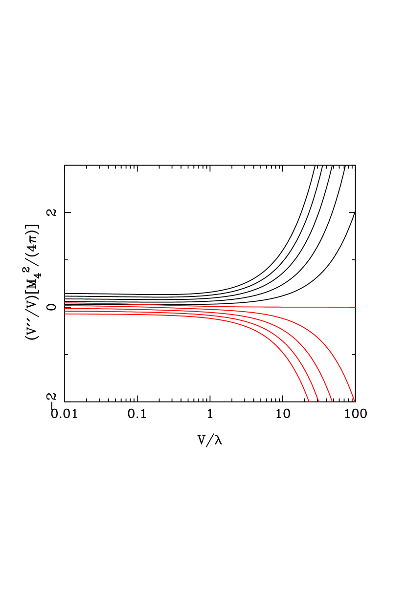
Figure 3: The recovered curvature of the inflaton potential in the braneworld scenario as a function $V/\lambda$. The upper set of five lines are for $R=0.01$ to $0.05$, with $n-1=0$, while the lower set are from the same range of $R$ with $n-1=-0.2$.

Finally we demonstrate these degeneracies for an example set of observables. We choose our observables to be $A_{T}^{2}=4\times 10^{-12}$, $R=0.01$, and $n-1=-0.05$; these numbers correspond roughly to the predictions from a quartic potential and are consistent with current observations WTZ (the ratio of contributions to the large-angle microwave anisotropies is about $4\pi R$ in our conventions). We reconstruct potentials for choices of $\lambda$ evenly spaced logarithmically in the range from $10^{-15}\,M_{4}^{4}$ to $10^{-9}\,M_{4}^{4}$. In each case, we plot only the portion of the potential accessible to observations; the relation between $\Delta\phi$ and the range of scales probed by observations depends on $\lambda$ and is computed via Eq. (7) as

$$\frac{\Delta\phi/M_{4}}{\Delta\ln k}=\sqrt{\frac{R}{4\pi}}\;\frac{1}{G(\tilde{V})}\,.$$ (29)

We take the Planck satellite as our guideline, which will have $\Delta\ln k\simeq 3.5$ on either side of the central point.

Figure 4: Different potentials as obtained for the different choices of $\lambda$ described in the text, with the highest curves corresponding to the highest $\lambda$. Einstein gravity is recovered as $\lambda\rightarrow\infty$. Each potential generates the same initial spectra.

Figure 4 shows a set of reconstructed model potentials for the different assumed values of $\lambda$, each of which reproduces our model observations. The ratio $V/\lambda$ obtained ranges from $0.01$ to $22$. For $V\ll\lambda$ the reconstructed potential is nearly independent of $\lambda$, closely approximating the Einstein gravity result. As $\lambda$ is decreased, the magnitude of the potential begins to decrease while its gradient steepens; at the same time the amount of potential constrained shrinks as the extra friction leads to slower rolling of the field.

To end, we mention that as well as reproducing the correct perturbations, a viable potential must be able to support enough subsequent inflation to stretch those perturbations to the observable scales. If the recovered potential develops a minimum or goes negative within the constrained range, our approach will have broken down, and refinement becomes necessary (going beyond the quadratic potential approximation and/or slow-roll) to test whether there is still a viable potential. However the approximate condition for the reconstruction to break down, $\Delta\phi\gtrsim|V^{\prime}/V^{\prime\prime}|$, does not change significantly as $\lambda$ is decreased, because in the high-energy limit $\Delta\phi$ reduces at the same rate as $V^{\prime}/V^{\prime\prime}$ (for fixed values of the observables). Hence if a viable potential exists in the $\lambda\rightarrow\infty$ limit, it is unlikely that the problem will become ill-defined for low values of $\lambda$.

III Conclusions

One of the most anticipated results of forthcoming high-accuracy CMB experiments is the probing of the physics of inflation, and in particular empirically reconstructing the form of the inflaton potential. However, it is important to be aware of the possible degeneracies that may arise. To date attention has been focussed on degeneracies between initial perturbation parameters and cosmological parameters such as reionization, suggesting that combinations of observations (for example CMB polarization as well as temperature, or completely different types of observation) are required to lift these degeneracies.

For early Universe cosmologists, more worrying are degeneracies that arise in predictions for the initial perturbations, which represent a fundamental limitation to the constraints we can extract and which are not broken by polarization. In this paper we have described how such a degeneracy arises in a braneworld scenario based on the Randall–Sundrum type-II model. We have shown that the unique reconstruction of the potential from scalar and tensor perturbation spectra in this scenario is no longer possible, with a different possible potential arising for each choice of brane tension. Accordingly, observations of the perturbation spectra cannot distinguish between the braneworld and standard inflation. It would be interesting to know if this is unique to the simplest braneworld scenario, or if it remains true in other versions. It would also be interesting to know if this result persists at higher order in the slow-roll expansion for the perturbations.

We end by stressing that our results refer to the initial perturbation spectra. Whether or not there might be significant braneworld effects on the subsequent evolution of the perturbations is presently unknown and is likely to be model dependent; for example in general the short-scale perturbation behaviour on the brane can be influenced by bulk perturbations which cannot be predicted on the brane (see Ref. Maartens for an overview). It may well be that the braneworld might manifest itself through such effects. If, however, the perturbation evolution turns out to be unaffected (for example if inflation is successful in diluting the effect of bulk perturbations), then finding observable traces of the braneworld in the low-energy universe may not be easy.

- (1) A. R. Liddle and D. H. Lyth, Cosmological Inflation and Large-Scale Structure, Cambridge University Press, Cambridge, 2000.
- (2) E. J. Copeland, E. W. Kolb, A. R. Liddle, and J. E. Lidsey, Phys. Rev. D48, 2529 (1993) [hep-ph/9303288].
- (3) J. E. Lidsey, A. R. Liddle, E. W. Kolb, E. J. Copeland, T. Barreiro, and M. Abney, Rev. Mod. Phys. 69, 373 (1997) [astro-ph/9508078].
- (4) P. Binétruy, C. Deffayet, and D. Langlois, Nucl. Phys. B565 (2000) 269 [hep-th/9905012]; P. Binétruy, C. Deffayet, U. Ellwanger, and D. Langlois, Phys. Lett. B477, 285 (2000) [hep-th/9910219].
- (5) T. Shiromizu, K. I. Maeda, and M. Sasaki, Phys. Rev. D62, 024012 (2000) [gr-qc/9910076].
- (6) L. Randall and R. Sundrum, Phys. Rev. Lett. 83, 4690 (1999) [hep-th/9906064].
- (7) R. Maartens, D. Wands, B. A. Bassett, and I. P. C. Heard, Phys. Rev. D62, 041301 (2000) [hep-ph/9912464].
- (8) D. Langlois, R. Maartens, and D. Wands, Phys. Lett B489, 259 (2000) [hep-th/0006007].
- (9) G. Huey and J. E. Lidsey, astro-ph/0104006.
- (10) A. N. Taylor and A. Berera, Phys. Rev. D62, 083517 (2000) [astro-ph/0006077].
- (11) X. Wang, M. Tegmark, and M. Zaldarriaga, astro-ph/0105091.
- (12) R. Maartens, gr-qc/0101059.