Voids in the PSCz Survey and the Updated Zwicky Catalog

Abstract

We describe an algorithm to detect voids in galaxy redshift surveys. The method is based on the void finder algorithm of El-Ad & Piran. We apply a series of tests to determine how accurately we are able to recover the volumes of voids using our detection method. We simulate voids of different ellipticity and find that if voids are approximately spherical, our algorithm will recover 100% of the volume of the void. The more elliptical the void, the smaller the fraction of the volume we can recover. We insist that voids lie completely within the survey. Voids close to the edge of the survey will therefore be underestimated in volume. By considering a deeper sample, we estimate the maximal sphere diameters are correct to within 30%.

We apply the algorithm to the Point Source Catalogue Survey (PSCz) and the Updated Zwicky Catalog (UZC). The PSCz survey is an almost all-sky survey with objects selected from the IRAS catalog. The UZC covers a smaller area of sky but is optically selected and samples the structures more densely. We detect 35 voids in the PSCz and 19 voids in the UZC with diameter larger than 20$h^{-1}$Mpc. Using this minimum size threshold, voids have an average effective diameter of 29.8$\pm 3.5h^{-1}$Mpc (PSCz) and 29.2$\pm 2.7h^{-1}$Mpc (UZC) and that they are underdense regions with $\delta\rho/\rho$ values of -0.92$\pm 0.03$ (PSCz) and -0.96$\pm 0.01$ (UZC) respectively. Using this quite stringent threshold for void definition, voids fill up to 40% of the volume of the universe.

1 Introduction

The distribution of galaxies in redshift surveys reveals vast regions of space that seem to be avoided by galaxies. These are termed voids, although voids may not be completely empty, but may harbor a few isolated galaxies. During the 1970’s, the use of galaxy redshift surveys to trace the large scale structure began in earnest. Gregory & Thompson (1978) showed evidence for the existence of superclusters and void regions with radii larger than 20$h^{-1}$Mpc using pencil beam surveys directed toward the Coma and Perseus cluster. Einasto, Joeveer & Saar (1980) discuss the chain-like distribution of galaxies and galaxy clusters and the existence of empty cell structures. Kirshner et al. (1981) discovered a void in Boötes that is 50$h^{-1}$Mpc in diameter. The ubiquity of voids and their importance in the large scale distribution of galaxies was first clearly shown by results from the Center for Astrophysics surveys (Davis et al. 1992; de Lapparent, Geller, & Huchra 1986; Geller & Huchra 1989) and the Southern Sky Redshift survey (da Costa et al. 1988, 1994; Maurogordato et al. 1992). Subsequent larger surveys at a variety of wavelengths have confirmed these results and have shown that no larger voids are seen at similar density contrast. See the review article by Rood (1998) and references therein for a discussion of the history of void detection and interpretation.

Voids appear to have little or no structure within them. Peebles (2001) discusses an apparent discrepancy between the cold dark matter model and observations. The cold dark matter model predicts that there should be matter and, hence galaxies, primarily dwarfs, within voids (Dekel & Silk 1986; Hoffman, Silk & Wyse 1992). However, studies of different types of galaxies show that they all seem to trace the same structures. Grogin & Geller (1999, 2000) identify a sample of void galaxies in the CfA2 survey and find evidence for environmental dependence of galaxy properties, although most of these galaxies in this sample avoid the centers of the voids. Surveys of dwarf galaxies indicate that they trace the same overall structures as ‘normal’ galaxies (Bingelli 1989) and pointed observations toward void regions also fail to detect a significant population of faint galaxies (Kuhn, Hopp & Elsässer 1997; Popescu, Hopp & Elsässer 1997), consistent with the widely observed result that galaxies have common voids regardless of Hubble type (e.g. Thuan, Gott & Schneider 1987; Babul & Postman 1990; Mo, McGaugh & Bothun 1994). Whether Lyman alpha clouds in voids are associated with galaxy halos or are a distinct population remains controversial (Lanzetta et al. 1995; Morris et al. 1993; see Stocke 2001 for further references). Either we are missing a population of galaxies that reside in the voids or the CDM models produce too much clustering of matter on small scales (Bode, Ostriker & Turok 2001). The sizes of voids have also been used to place constraints on CDM models. Blumenthal et al. (1992) and Piran et al. (1993) find that the frequency and size of voids detected in redshift surveys are difficult to reconcile with CDM models unless the Universe is open or that galaxies do not trace mass on very large scales.

There are several different algorithms in the literature for detecting voids (see, for example, Kauffmann & Fairall 1991; Kauffmann & Melott 1992; Ryden 1995; Ryden & Melott 1996; El-Ad & Piran 1997 (EP97); Aikio & Mähönen 1998) but due to the large diameter of voids (their characteristic diameter is as large as 50 $h^{-1}$Mpc) and the limited volume of most surveys, relatively few voids have been objectively detected. A search for voids has so far been made using the first slice of the Center for Astrophysics Survey (Slezak, de Lapparent & Bijaoui 1993), the Southern Sky Redshift Survey (Pellegrini, da Costa & de Carvalho 1989; El-Ad, Piran & da Costa 1996, EPC96), the IRAS 1.2 Jy Survey (El-Ad, Piran and da Costa 1997, EPC97), the Las Campanas Survey (Müller et al. 2000) and the PSCz Survey (Plionis & Basilakos 2001). Voids were detected in the CfA slice and the Las Campanas Survey, restricted to two-dimensions due to the small declination range of each data set. Eleven voids with $>$95% significance have been detected in the SSRS2 survey (EPC96), twelve voids with $>$95% significance have been detected in the IRAS 1.2-Jy Survey (EPC97) and fourteen voids with volumes larger than $10^{3}h^{-3}$ Mpc³ have been detected in the PSCz Survey (Plionis & Basilakos 2001). Statistically, voids have also been studied using the Void Probability Function (VPF, White 1979) and the Underdensity Probability ($U(R)$, Vogeley et al. 1989), which depend on the hierarchy of n-point correlation functions. The VPF is simply the probability that a randomly selected volume contains no galaxies. The $U(R)$ measures the frequency of regions with density contrast $\delta\rho/\rho$ below a threshold. These statistics reveal statistical information about the void population but do not give details on specific voids.

A first step in rectifying our relative neglect of voids is to quantitatively characterize their properties, as defined by surveys at different wavelength. Here we adapt the approach of EP97 in order to search for voids in the PSCz Survey (Saunders et al. 2000) and the Updated Zwicky Catalog (UZC, Falco et al. 1999). We describe the surveys in Section 2 and describe the algorithm in Section 3. We present our results and draw conclusions in Section 4 and 5 respectively.

2 The Surveys

We consider two surveys with different wavelength selection to see if the same voids are detected and if the properties of voids in overlap regions are similar (see Section 4.2). We consider different samples from the two surveys to check the robustness of results. In particular we are able to check the effect of the wall/field criteria on the detection of voids (see Section 4.5) and by how much the volume of voids is restricted by the sample depth (see Section 4.6).

2.1 The Updated Zwicky Catalog

The Updated Zwicky Catalog (Falco et al. 1999) includes a re-analysis of data taken from the Zwicky Catalog and Center for Astrophysics redshift survey to $M_{Zwicky}\mathrel{\hbox{\hbox to0.0pt{\hbox{\lower 4.0pt\hbox{$\sim$}}\hss}\hbox{$<$}}}$ 15.5 (Zwicky et. al 1961-1968; Geller & Huchra 1989; Huchra et al. 1990; Huchra, Geller & Corwin 1995; Huchra, Vogeley & Geller 1998 ) together with new spectroscopic redshifts for some galaxies and coordinates from the digitized POSS-II plates. Improvements over the previous catalogs include estimates of the accuracy of the CfA redshifts and uniformly accurate coordinates at the $<2^{\prime\prime}$ level. The UZC contains a total of 19,369 galaxies. Of the objects with m${}_{Zwicky}\mathrel{\hbox{\hbox to0.0pt{\hbox{\lower 4.0pt\hbox{$\sim$}}\hss}\hbox{$<$}}}15.5$, 96% have measured redshifts, giving a total number of 18,633 objects. The catalog covers two main survey regions; $20^{h}<\alpha_{1950}<4^{h}$ and $8^{h}<\alpha_{1950}<17^{h}$ both with $-2.5^{\circ}<\delta_{1950}<50^{\circ}$.

We consider three different samples from the catalog. We construct a volume-limited sample with $z_{\rm max}$=0.025 corresponding to a depth of 74$h^{-1}$Mpc, for an Einstein-de Sitter cosmology. The absolute magnitude of each galaxy is estimated to be

$$M=m_{Zwicky}-25-5{\rm log}[r(1+z)]-3z$$ (1)

and this sample is limited to $M_{lim}=-18.96$. Previous analyses of the CfA or UZC samples have removed areas in the South Galactic Cap region with extinction larger than $\Delta m\mathrel{\hbox{\hbox to0.0pt{\hbox{\lower 4.0pt\hbox{$\sim$}}\hss}\hbox{$>$}}}0.3$. We do not apply this cut as it severely restricts the volume of the survey. Instead, we compare the voids we find in the UZC with those we find in PSCz to examine if the paucity of galaxies in these regions of the catalog causes us to falsely detect voids.

This volume-limited sample contains 3518 galaxies, which is the largest number of galaxies in a volume limited sample that can be constructed from the catalog. Application of the wall/field criteria (defined in Section 3.2) to this sample yields 3240 wall galaxies and 278 field galaxies. We also consider the same volume limited sample without applying the wall/field criteria to see how the voids are affected when we insist they are completely empty. We also consider a sample that extends an extra 20$h^{-1}$Mpc in depth to estimate the impact of the survey boundary on the estimated sizes of voids.

2.2 The PSCz Survey

Objects in the PSCz Survey were selected from the IRAS Point Source Catalog (Beichman et al. 1984) which is a catalog of detections down to a flux limit of 0.6 Jy taken with the IRAS (Infra-Red Astronomical Satellite). Targets for the PSCz survey were chosen to maximise the sky coverage but at the same time other considerations such as completeness, flux uniformity, having a well defined sample area and redshift range were taken into account. (See Saunders et al. 2000 and references therein for a more complete description of target selection criteria.)

The PSCz survey covers 84% of the sky. Areas with incomplete IRAS data and high optical extinction, such as the plane of the Galaxy, are not included in the Survey. The PSCz survey contains 15,411 galaxies. Of order 8,000 objects had known redshifts in the literature (Saunders et al. 2000). Follow-up observations were carried out to obtain the remaining redshifts. The median redshift of the survey is 0.028 corresponding to a comoving depth of $\sim 80h^{-1}$Mpc assuming an EdS cosmology.

In a flux limited sample the number density of detectable objects decreases with distance. Thus, we are more likely to detect voids towards the edge of the survey because the average galaxy-galaxy separation increases. Therefore we restrict the depth of the sample to the median redshift, 0.028, which closely matches the depth of the UZC sample. As IR selected surveys are sparse compared to optically selected surveys, we keep all the galaxies in the sample, i.e. we do not construct a true volume-limited catalog. We find that void properties do not vary with depth over the range we consider, thus the void finding algorithm is robust with respect to small changes in the selection function. The average density of objects in this PSCz sample is comparable to the density of objects in the volume-limited UZC sample if we do not apply the volume limited criteria to PSCz. This allows us to compare voids found in the two surveys at similar sampling density.

As for the UZC, we consider this sample in two ways, one where we we apply the wall/field galaxy criteria (defined in Section 3.2) and one where we do not (and so all galaxies are wall galaxies). This sample contains 8425 galaxies (7743 wall galaxies and 682 field galaxies) A third sample is constructed in which we extend the sample by 20$h^{-1}$Mpc. Again, this is to examine by how much we underestimate the volume of voids when we impose our cut in depth.

3 The Void Finding Algorithm

3.1 Outline

Here we outline the steps involved in our void finding algorithm. Each of the steps are discussed in detail in the subsequent sections. The void finding algorithm we adopt is very similar to the method used by El-Ad & Piran (Void Finder EP97, EPC97).

Tests with toy model distributions and results of N-body simulations indicate that this algorithm is robust in locating voids and measuring their sizes. The method allows for “field galaxies” in the voids, which are removed before void detection. This step ensures that void detection is not dominated by shot noise of the few galaxies in these large underdensities. Setting a minimum void size prevent voids from percolating through small gaps in the dense wall-like or filamentary structures. This minimum void size is also set so that the voids are statistically significant in comparison with randomly occurring holes in a Poisson distribution with the same average density of objects. As long as the sampling density is high enough that the overdense structure are well-defined (no gaps comparable to or larger than the minimum void threshold), then void detection is not highly sensitive to the sampling density.

The steps of the void finding algorithm are as follows:

• Classification of galaxies as wall or field galaxies, Section 3.2

• Detecting empty cells in the distribution of wall galaxies, Section 3.3

• Growth of the maximal empty spheres, Section 3.4

• Classification of the unique voids, Section 3.5

• Enhancement of the void volume, Section 3.6

3.2 Wall and Field Galaxies

The first stage in identifying voids is to determine which galaxies are classed as field galaxies and which are wall galaxies. Here we follow the method of EP97. First we calculate the mean distance, d, to the $n^{\rm th}$ galaxy and the standard deviation on this value, $\sigma$. We then specify a length l_n such that any galaxy that does not have $n$ neighbours within a sphere of radius l_n is classified as a field galaxy. The value of l_n we adopt is given by l_n = d + 1.5$\sigma$ and we set $n$=3. For our main samples, the values of d and l₃ that we obtain for the PSCz survey are 3.42$h^{-1}$Mpc and 7.19$h^{-1}$Mpc respectively while for the UZC we obtain 3.46$h^{-1}$ and 6.52$h^{-1}$Mpc. This choice of sphere size means that field galaxies are found in regions with density contrast, $\delta\rho/\rho$, of less than -0.5. For n=3 $\sim$10% of galaxies are classified as field galaxies in both surveys. If $n$=0 then all the galaxies are field galaxies and the survey is just one large void (or two because of the disjoint geometry of both the PSCz and UZC). If $n$ is higher than 3, then the proportion of galaxies classified as field galaxies drops rapidly. We compare results for our main sample to an analysis of a sample where all the galaxies are classed as wall galaxies to see what effect the exclusion of field galaxies has on the voids we detect.

We also have to consider what effect the edges of the survey have on our wall/field criteria. Galaxies close to the edges may appear isolated and be classified as field galaxies but they may be part of large groups just outside the geometry of the sample under consideration. This could lead to a slight overestimation of the size of the voids near the survey boundary because a maximal sphere in the vicinity of an erroneously classified edge galaxy can be grown to the survey boundary rather than being bounded by that galaxy. As these wrongly classified field galaxies are only those close to the survey edge, the maximal spheres cannot be grown much larger and hence the void sizes should not be overestimated by a large amount. There is no indication that voids near the boundaries are larger than those interior to the surveys.

Similarly, we may overestimate the values of $\delta\rho/\rho$ for voids that lie close to the edges as the wrongly classified field galaxies may lie within a void. However, on inspection, few of these galaxies actually lie in voids due to the spherical nature of voids and the proximity of the survey boundary.

Figure 1: The void finder technique. The method is discussed in more detail in the text. Step 1, we identify an empty cell within a void. From that cell we find the nearest wall galaxy and grow the sphere to that radius. Step 2, we move away from the first galaxy, growing the sphere until the second galaxy is on the surface. Step 3, we connect the sphere center to the point which bisects the two detected galaxies and move the center along this vector until a third galaxy is on the radius. In 2D this is where we stop. In 3D, the final stage is to move the sphere center out of the plane defined by the first three galaxies. The open squares in the diagrams are previous void centers and earlier detected galaxies. The solid squares show the current void center and the galaxy detected at each stage. The points in this two dimensional example are randomly generated in a box with a circular area carved out as a demonstration of the technique.

3.3 Detecting the Empty Cells

The next step is to place the galaxies (either all the galaxies or just the wall galaxies when we apply the wall/field criteria) onto a three dimensional grid and count the number of galaxies in each cell. Cells that lie at a greater distance than the maximum radius of the sample under consideration are not considered further. The fineness of the grid defines the minimum size void that can be detected. If each grid cell has length l_cell, then voids with radius r = $\sqrt{3}$l_cell will be found. We fix l_cell to be the same as l₃.

3.4 Growth of the Maximal Spheres

Each empty grid cell (we will refer to these as holes) is considered to be part of a possible void. Our method finds the maximal sphere that can be drawn in the void, starting from the empty cell, and is shown schematically in Figure 1. From the center of the empty cell, we grow a sphere, increasing its radius until we find a galaxy that is just on the edge of it. We then find the vector that connects this galaxy with the center of the hole and move the center of the spherical hole along this direction, away from the first galaxy, growing the radius to keep the first galaxy on its surface, until a second galaxy is also on the surface. We next find the vector that bisects the line joining the two galaxies and move the hole in this direction until a third galaxy is found, as before. If voids are being detected in two dimensional data, the process stops here. However, we are considering three dimensional data so the final step is to grow the hole out of the plane formed by the first three galaxies. We insist that our voids lie completely in the survey i.e. they are contained within the volume specified by our survey boundaries and sample depth. At this stage we keep track of all the holes with radii larger than the value of the search radius used to classify field and wall galaxies, $l_{3}$.

Our method is somewhat redundant. We specify the minimum size of our holes that form voids but many voids are far larger than this and more than one empty cell may lie within the void region, thus we grow some voids more than once. However, it does guarantee that we find all the holes that can contribute to the voids volume so the redundancy is eliminated when we calculate the volume of the voids (see Section 3.6).

3.5 Classification of Unique Voids

Finding the holes is a robust process. Deciding which of those holes are unique voids requires more care. Our definition of a void is slightly different from that of EP97. First we sort the holes by radius, the largest first. The largest hole found is automatically a void. We define a fractional overlap parameter, $\eta_{1}$. If the second void overlaps the first by more than $\eta_{1}$ in volume, then we say it is a member of the first void rather than a new void. If not then it forms a separate void. We then check the third hole to see if it overlaps either of the previous voids by $\eta_{1}$ in volume. If it does, we add it to that void; if not, we form a new void. If it overlaps two voids by more than $\eta_{1}$ then we reject the hole as it links two larger, independent voids. We continue like this for all holes with radii larger than 10$h^{-1}$Mpc.

We have investigated how much holes should overlap and yet be considered separate voids. If the overlap threshold is high, say $\eta_{1}$=90%, then most of the holes are considered unique voids and the same empty region may be contained in more than one void. If the overlap fraction is too low, then voids that barely overlap are considered two parts of the same void. This means that if there are any small gaps in the walls, two spheres could be joined together to form a single void which, under visual inspection, obviously consists of two voids.

In figure 2 we show the number of voids we find for the PSCz (dashed line) and the UZC (solid line) as we vary the percentage overlap. The values seem to flatten off for $\eta_{1}<$30%. We fix the value of $\eta_{1}$ to be 10%. Visually, using our criteria of $\eta_{1}$=10%, voids appear to be distinct regions of the survey. For a void with a radius of 10$h^{-1}$Mpc and with an overlap region of $\eta_{1}$=10%, gaps in the walls would have to be larger than 9$h^{-1}$Mpc, which is larger than the wall/field galaxy criteria and larger than the average galaxy-galaxy separation in both surveys. Gaps of this size in the walls are rare so distinct voids are not connected. Therefore, if a hole with radii larger than 10$h^{-1}$Mpc overlaps a larger void by more than 10% of its volume, we merge the hole into that void. If $\eta_{1}$ is less than 10% of the smaller void’s volume, we deem the sphere to be a distinct void and if the hole overlaps two larger voids by 10% we reject it.

Figure 2: The number of voids in each survey as a function of overlap fraction, $\eta_{1}$, allowed between distinct voids (dashed line PSCz, solid line UZC). If spheres are allowed to almost completely overlap and still be classified as individual voids, then we detect too many voids in each survey. We adopt a value of $\eta_{1}=$10%.

We set a threshold of 10$h^{-1}$Mpc for the minimum size of voids. This threshold is larger than the search radius for defining field galaxies, $l_{3}$. This helps ensure that we do not identify gaps in the walls as voids. It is also the value at which the significance of detecting voids in the both the PSCz and UZC catalog drops below 95%, discussed in Section 4.1.

3.6 Enhancement of the Void’s Volume

We next enhance the volume of each void. We consider the holes that have radii less than the threshold of 10$h^{-1}$Mpc but greater than the radius for the wall/field galaxy criterion, l₃, (in the case where we do not make the wall/field galaxy cut we still use l₃ as the minimum sphere radius). Any hole that overlaps the maximal void sphere (as grown in Section 3.4) by $\eta_{2}>$50% of the smaller hole’s volume is also considered part of the larger void. If the hole overlaps with more than one void then it is not added to either of the voids as this would link two voids together that we wish to keep separate. If the hole is isolated it cannot be classed as a separate void as it is smaller than the threshold we use for void classification. The choice of $\eta_{2}=$50% is somewhat arbitrary but it fills the void volume without changing the overall spherical shape of the voids. We have compared the volumes of voids found using different values of $\eta_{2}$. For values of $\eta_{2}$ in the range 20-70%, the volumes of voids are robust to within 20%.

We compute the volume of each void by Monte Carlo integration, i.e. we embed it in a box that is larger than the void and generate many random particles within the box and count how many lie within one of the holes that make up the void. The ratio of the number of randoms in the void to the total number of randoms placed in the box multiplied by the volume of the box gives an estimate of the volume of the void. We could, in principle, calculate the volume of the void analytically as it is just formed by a series of overlapping spheres. However, if a void consists of more that three overlapping holes, the solution is rather complicated.

We are likely to underestimate the volumes of voids as we only consider holes that have radius greater than the search radius, $l_{3}$. If voids are highly elliptical then we will not detect the volume at the ‘corners’ of the ellipse. We test this by generating data containing mock voids of known elliptical shape. We take the average volume of a void, taken to be 15,000$h^{-3}$Mpc³, and generate ellipsoids with this volume that have axis ratios 1:1:X (i.e. if X is 1 then the void is spherical with radius 15.3$h^{-1}$Mpc). We then run the simulated data through our void finding algorithm and compare the volume obtained with the known volume of the void. The results are shown in Figure 3. If voids are spherical in shape then we recover 100% of its volume. The more elongated it becomes, the less of the volume we detect. This becomes significant if one of the axes is elongated by more than a factor of 2.5 than the others. If the axis are in the ratio 1:1.5:2 then we can recover 90% of the volume and if they are in the ratio 1:2:3 we can recover 70% of the volume. As voids are seen to be roughly spherical in nature we should be able to detect most of a void’s volume.

Finally in the case where we specify wall and field galaxies, we count the number of field galaxies that lie in each void to determine the underdensity of the void.

Figure 3: The accuracy to which we recover the volume of an ellipsoid with axis ratios 1:1:X. If the void is spherical then we recover 100% of the volume of the sphere. The more elongated the void, the smaller the fraction of the volume we recover when requiring that the maximum sphere size be larger than the wall/field criteria, $l_{3}$. We only show the results for ellipses with two axes equal and the third different as this is the worst case scenario. If the axis are in the ratio 1:1.5:2 we recover 90% of the volume and if they are in the ratio 1:2:3 we recover 70% of the volume.

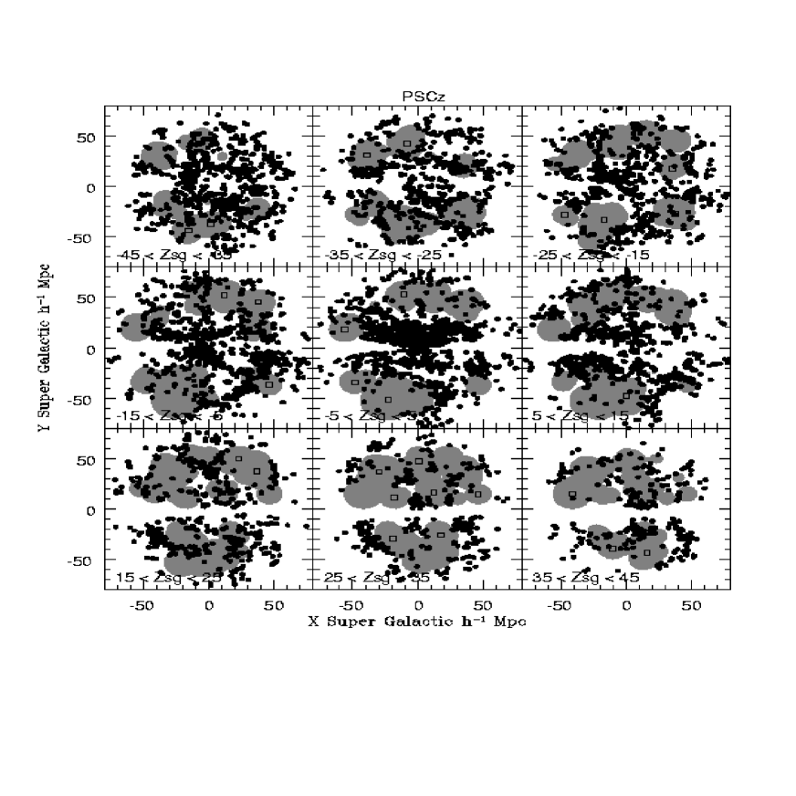
Figure 4: Voids in the PSCz Survey. We show the supergalactic coordinates (X,Y) for different values of Z. Each panel shows a 10$h^{-1}$Mpc slice starting at -45$h^{-1}$Mpc$<$Z$<$-35$h^{-1}$Mpc top left to 35$h^{-1}$Mpc$<$Z$<$45$h^{-1}$Mpc bottom right. The shaded regions are the voids. The filled points are the wall galaxies and the open squares show the void centers (as the voids have radii $>10h^{-1}$ Mpc they spread over more than one panel and thus some shaded areas do not contain a void center). No wall galaxies are found in the voids. Field galaxies are not shown.

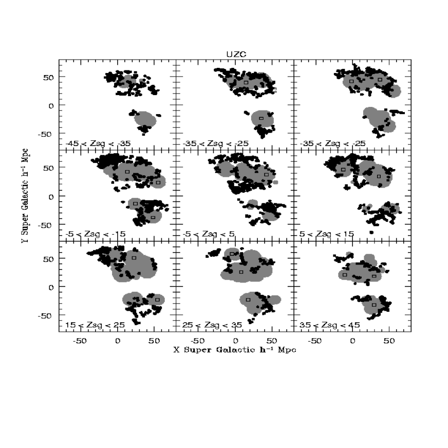
Figure 5: Voids in the UZC Survey. We show the supergalactic coordinates (X,Y) for different values of Z. Each panel shows a 10$h^{-1}$Mpc slice starting at -45$h^{-1}$Mpc$<$Z$<$-35$h^{-1}$Mpc top left to 35$h^{-1}$Mpc$<$Z$<$45$h^{-1}$Mpc bottom right. The shaded regions are the voids. The filled points are the wall galaxies and the open squares show the void centers (as the voids have radii $>10h^{-1}$ Mpc they spread over more than one panel and thus some shaded areas do not contain a void center). No wall galaxies are found in the voids. Field galaxies are not shown.

Figure 6: The left hand plot shows a comparison between the radii of the maximal sphere and the volume of voids detected in both the PSCz and UZC catalogue. The radii of the voids detected in the two surveys agree to with in 20%, indicating that sample selection plays little effect on the diameters of voids. The center and right hand plot give an indication of the amount we underestimate the radii of the maximal spheres (triangles) and the volumes (circles) of voids by insisting they lie entirely in the volume of the survey as a function of depth for the PSCz survey (center plot) and the UZC (right hand plot). Voids that lie closer to the depth boundary naturally suffer more from underestimation problems but even so, we estimate the radii are accurate to within 30%.

4 Results

Voids in the main PSCz and UZC sample are shown in Figure 4 (PSCz) and 5 (UZC). In both cases, the points represent the wall galaxies and the shadings represent areas that are covered by voids. Squares indicate the three dimensional center of each void. Projecting 3-D data onto a 2-D page makes the voids appear to contain galaxies but in reality voids are free from wall galaxies (but may contain field galaxies which are not shown). We find 35 voids with r$>10h^{-1}$Mpc in the PSCz survey and 19 voids with r$>10h^{-1}$Mpc in the UZC.

4.1 Significance of the Voids

We use the method of EPC97 to assess the significance of voids. The confidence level with which we detect a void is given by

$$p(r)=1-\frac{N_{\rm Poisson}(r)}{N_{\rm Survey}(r)}$$ (2)

where $N_{\rm Survey}(r)$ is the number of voids in the sample under consideration and $N_{\rm Poisson}$ is the number of voids found in Poisson realisations of the sample. These have the same number density of points and the same radial and angular selection functions of the sample but the points are unclustered. The closer $p(r)$ is to 1, the less likely a void could occur in a random distribution.

With a threshold of 10$h^{-1}$ Mpc for the void radius, we find an average of 1.9 voids in the mock PSCz realisations and an average of 1.1 voids in the UZC realisations. Thus the voids we detect in both the PSCz and UZC with radius $>$10$h^{-1}$ Mpc are significant at the 95% confidence level, which is why we set this minimum size threshold.

4.2 Sizes of the Voids

The largest hole in the PSCz survey has a diameter of 35.7$h^{-1}$Mpc, whereas in the UZC survey the largest hole has a diameter of 29.3$h^{-1}$Mpc. The wider angle covered by the PSCz survey allows somewhat larger voids to be detected. The average void in the PSCz survey has a maximal sphere diameter of 24.8$\pm 3.3h^{-1}$Mpc and an effective diameter of 29.8$\pm 3.5h^{-1}$Mpc (we find the effective diameter by calculating the diameter of a sphere that would match the volume of the void) whereas the average void in the UZC survey has a slightly smaller maximal sphere diameter of 23.6$\pm 2.7h^{-1}$Mpc and an effective diameter of 29.2$\pm 2.9h^{-1}$Mpc. The average void size obviously depends on the minimum size threshold of r$>$10$h^{-1}$ Mpc. Raising or lowering this threshold raises or lowers the average void size. The maximal spheres typically fill 60% of the void’s volume, found by dividing the volume of the void by the volume of the maximal sphere. There does not appear to be any trend with void size in this filling fraction.

We compare the voids detected in both the PSCz and the UZC. We are able to match 15 out of the 19 voids in the UZC to voids in the PSCz. Two (10 and 16 in the UZC list) of the voids detected in the UZC form one void in the PSCz survey. Void 19 appears to be a case where the maximal sphere in the PSCz survey lies just below the threshold of 10$h^{-1}$Mpc and so is not classed as a void in the PSCz. Voids 12 and 18 (marked with an asterisk in table 2) are found in areas with high extinction in the South Galactic Cap. There are few galaxies detected in the UZC in these regions so voids can be grown. As extinction is less of a problem in the IR, relatively more galaxies are detected in the PSCz sample and voids are not detected. Thus, these particular voids are suspect and we exclude them from calculation of the statistical properties of voids.

For the 15 voids that we do detect in both of the surveys, the diameter of the maximal spheres and the volumes we detect are very similar. In figure 6 we divide the diameters and volumes of the voids detected in the PSCz by the same values found from the UZC and find values fairly close to 1.

4.3 Density of Voids

In the case where we differentiate between wall and field galaxies, we can determine the density contrast of voids. We find that voids have a typical density contrast of $\delta\rho/\rho$ = -0.92$\pm 0.03$ in the case of the PSCz survey and -0.96$\pm 0.01$ in the case of the UZC survey. These values are very low; even with 10% of galaxies classed as field galaxies the field galaxies probably lie close to the structures traced by the wall galaxies and therefore are not detected within the void volume. Again, there is no trend seen between the underdensity and size of voids; the largest voids and the smallest voids all have consistent values of $\delta\rho/\rho$.

The total volume fraction occupied by voids in the PSCz and UZC surveys is 30% and 40% respectively. Compared to previous estimates, this value is low. De Lapparent, Huchra & Geller (1991) find that high density regions only fill 25% of the Center for Astrophysics slices, leaving up to 75% to be filled by lower density regions. The voids we detect are extremely low density voids, hence they fill a smaller fraction of the survey.

4.4 Comparison with other papers

We can compare results with voids detected by EPC97 in the 1.2 Jy Survey. The 1.2 Jy survey covers the same area as the PSCz survey but is sparser due to the higher flux limit. Consequently, fewer voids are found to the same significance level. 12 voids with $>95$% significance are found and these have an average diameter of 40$h^{-1}$Mpc. This is significantly larger that the voids we detect in the PSCz but voids must have a diameter larger than 25$h^{-1}$Mpc to be 95% significant, thus the smaller voids are not reported by EPC97. In most cases, we detect the same regions as voids as EPC97. We class void 7 in EPC97 as two separate voids because our sample includes fainter galaxies that restrict the growth of the maximal spheres. There are also two voids that EPC97 report as significant at the 80% level that we do not detect in the PSCz sample (voids 14 and 15 in EPC97).

A recent paper by Plionis & Basilakos (2001) examines voids in the PSCz survey. Voids are found by these authors using a smoothed apparent magnitude limited sample rather than the point distribution of galaxies and the paper concentrates on measuring the shapes of voids and making a comparison to various cosmological models. Plionis & Basilakos find 14 voids out to 80$h^{-1}$Mpc with volumes larger than 10${}^{3}h^{-3}$ Mpc; we find 23 such voids. 9 of the voids are detected using both methods. The remaining 5 voids lie at distances such that a void with a radius of $>10h^{-1}$Mpc would not fit fully in the survey geometry. The 14 voids that we detect but which Plionis & Basilakos do not detect appear to be surrounded by high density regions. The smoothing technique appears to smooth the galaxies into the voids, restricting the number of voids that can be detected.

4.5 No Field Galaxies

What happens if we do not remove field galaxies from the samples? In either the PSCz or the UZC Survey, we find that 90% of the same voids are detected whether or not we make the wall/field galaxy cut. As expected, we miss a couple of the voids when we do not classify galaxies in low density regions as field galaxies as they interrupt the growth of the maximal spheres, thus the spheres lie below the detection threshold of 10$h^{-1}$Mpc and the voids are not detected.

As the voids we detect when we make the wall/field galaxy cut are so empty ($\delta\rho/\rho$ = -0.92, -0.96), it is not surprising that there is relatively little difference between the voids detected with and without applying the wall/field galaxy criteria.

4.6 Edge Effects

We also compare the volumes of the voids found in our main sample with voids found in samples that extend 20$h^{-1}$Mpc in depth beyond the depth of our main samples. We compare the volumes of voids and diameters of maximal spheres in the center (PSCz) and right hand (UZC) plots in figure 6. This plot shows that in general we underestimate the volume of voids by a larger factor at larger distance. This is not unexpected as it is only voids found at large depth that should be affected by the survey depth limit. However, the diameter of the maximal spheres are in reasonable agreement and the diameters are found to be the same to within 20%.

D(Max-Sphere)	D(Equiv)	Volume	Distance	$\alpha$	$\delta$	$\delta\rho/\rho$	Max-Sphere
(h-1Mpc)	(h-1Mpc)	(h-3Mpc3)	(h-1Mpc)	degrees	degrees		Fraction
35.68	44.45	45992.1	56.34	355.0	-47.7	-0.91	0.52
31.34	37.12	26789.5	59.31	97.8	-50.5	-0.94	0.60
31.00	39.99	33496.0	54.44	224.9	-2.0	-0.92	0.47
30.02	31.28	16018.4	57.57	246.9	-19.6	-0.96	0.88
28.52	33.55	19773.2	59.22	242.4	33.9	-0.96	0.61
27.29	31.87	16955.0	52.01	256.8	0.9	-0.95	0.63
27.27	32.86	18585.3	58.63	334.3	4.8	-0.94	0.57
27.22	32.28	17606.6	56.80	61.1	-27.6	-0.92	0.60
26.88	28.85	12572.5	59.52	149.1	56.6	-0.90	0.81
26.83	36.78	26053.0	49.03	351.9	-21.1	-0.94	0.39
26.59	35.66	23749.8	41.18	34.0	-55.2	-0.99	0.41
26.41	34.71	21891.0	55.46	206.9	71.9	-0.95	0.44
26.08	32.09	17301.4	59.26	164.1	-29.3	-0.94	0.54
25.88	30.16	14357.5	58.90	209.4	-42.9	-0.93	0.63
25.73	29.27	13129.7	59.55	210.4	52.8	-0.97	0.68
24.44	31.89	16980.8	53.96	170.3	34.5	-0.92	0.45
24.10	31.15	15821.7	43.60	310.6	-29.4	-0.96	0.46
24.03	31.27	16012.0	49.65	159.7	5.3	-0.95	0.45
23.78	30.58	14976.6	53.82	192.8	15.9	-0.91	0.47
23.68	32.14	17384.9	52.11	49.3	15.0	-0.90	0.40
23.53	25.72	8905.3	59.24	316.0	-74.1	-0.95	0.76
23.38	26.02	9224.0	54.02	85.1	-6.1	-0.95	0.73
23.22	26.70	9965.7	58.41	51.5	-46.0	-0.91	0.66
22.90	26.02	9223.6	59.03	285.5	47.1	-0.88	0.68
22.82	27.82	11273.7	38.63	263.4	43.6	-0.96	0.55
22.54	24.24	7462.0	33.63	250.3	-5.6	-0.94	0.80
22.47	27.01	10322.9	56.80	317.2	-15.7	-0.96	0.57
22.14	26.66	9923.2	58.08	124.2	6.8	-0.96	0.57
21.09	24.57	7764.9	43.66	102.5	48.6	-0.97	0.63
20.97	20.83	4731.8	56.08	311.6	73.4	-0.86	1.02
20.95	26.36	9594.2	56.45	223.1	31.7	-0.93	0.50
20.66	27.51	10899.4	42.51	332.4	15.9	-1.00	0.42
20.50	23.26	6586.8	59.68	27.5	21.4	-1.00	0.69
20.38	22.60	6047.6	46.97	91.5	-22.2	-1.00	0.73
20.21	21.26	5034.4	58.53	58.1	-84.8	-0.96	0.86

Table 1: The voids in the PSCz survey, with a distance cut of r $<80h^{-1}$Mpc, where field galaxies are differentiated from wall galaxies. We give (reading left to right) the diameter of the maximal sphere detected in the void, the equivalent diameter assuming the volume of the void is spherical, the volume of the void, the location of the void in distance, $\alpha$ and $\delta$ coordinates assuming an Einstein-de Sitter Universe, the density contrast of voids and the ratio of the volume of the largest hole to the total void volume.

D(Max-Sphere)	D(Equiv)	Volume	Distance	$\alpha$	$\delta$	$\delta\rho/\rho$	Max-Sphere
(h-1Mpc)	(h-1Mpc)	(h-3Mpc3)	(h-1Mpc)	degrees	degrees		Fraction
29.31	39.73	32828.0	51.22	197.8	73.9	-0.95	0.40
28.91	36.12	24667.1	42.09	247.2	39.8	-0.95	0.51
27.31	33.79	20204.3	49.81	52.1	15.8	-0.97	0.53
27.14	32.22	17506.9	59.56	209.7	52.6	-0.97	0.60
25.20	33.92	20443.4	44.54	168.0	38.3	-0.96	0.41
24.83	29.25	13104.5	49.15	254.4	13.7	-0.97	0.61
23.94	28.20	11747.8	59.68	332.5	21.8	-0.96	0.61
23.55	27.63	11045.8	47.74	196.6	12.2	-0.95	0.62
23.17	26.75	10025.9	38.91	334.5	18.6	-0.96	0.65
23.00	29.63	13625.9	61.75	136.9	48.4	-0.97	0.47
21.49	26.29	9509.8	45.36	162.6	14.7	-0.96	0.55
21.18*	23.89	7142.6	61.65	3.7	42.0	-0.97	0.70
21.07	24.15	7378.5	63.02	32.5	19.7	-0.95	0.66
20.93	25.54	8723.1	60.93	256.2	41.7	-0.97	0.55
20.79	26.23	9454.6	51.65	277.2	57.5	-0.95	0.50
20.55	26.78	10060.5	56.82	139.4	65.1	-0.97	0.45
20.54	23.72	6990.5	62.58	212.2	26.4	-0.97	0.65
20.28*	21.07	4901.1	30.35	48.6	21.9	-0.97	0.89
20.20	26.91	10203.0	51.07	141.2	25.4	-0.95	0.42

Table 2: The voids in the UZC, with a distance cut of r $<73.6h^{-1}$Mpc, where field galaxies are differentiated from wall galaxies. We give (reading left to right) the diameter of the maximal sphere detected in the void, the equivalent diameter assuming the volume of the void is spherical, the volume of the void, the location of the void in distance, $\alpha$ and $\delta$ coordinates assuming an Einstein-de Sitter Universe, the density contrast of voids and the ratio of the volume of the largest hole to the total void volume. The two voids marked with an asterisk are discussed in the text.

5 Conclusions

We have developed and tested a void finding algorithm, similar to that of EP97, and applied it to the PSCz and UZC surveys. Our method differs slightly from that of EP97 in the criteria that we use to identify unique voids; there is no obvious definition of how to group holes into voids. We demonstrate that our technique gives robust results in the sense that different samples from the same survey yield the same voids and we detect similar voids from redshift surveys with different wavelength selection. As an extension to the work of EP97 and EPC97 we quantify the effect of our void definition on the number of voids detected within a survey and we provide estimates of how accurately we are able to recover the volume of voids. We determine that the diameters of the voids presented here are probably accurate to within 20%. Detecting voids with relative densities of $\delta\rho/\rho=-0.92$, we find that up to 40% of the volume in the surveys under consideration is found in void regions. This is consistent with the findings of EPC97 and shows that voids are indeed a large part of the universe.

The next generation of surveys, the 2dF Galaxy Redshift Survey (Colless et al. 2001 and references therein) and, in particular, the Sloan Digital Sky Survey (York et al. 2000 and references therein) will aid our understanding of voids. Both of these surveys cover a larger sky area than the UZC, although not quite as large an area as the IR surveys. The SDSS will cover a quarter of the sky in one contiguous area which will be especially useful for void detection. Both the 2dFGRS and the SDSS will reach fainter magnitude limits than previous surveys, approximately 4 magnitudes deeper than the UZC. This will allow us to construct volume limited samples with more galaxies, which extend to greater depths. Perhaps more importantly, the multiband digital photometry, as well as the deep spectroscopy, of the SDSS will also allow us to study the properties of the field galaxies in detail. We will have a large enough sample of galaxies found in low density environments to statistically check if they have different properties than the galaxies found in the wall regions, allowing the role of environment on galaxy properties and formation to be examined.

References

- (1) Aikio, J., & Mähönen, P. 1998, ApJ, 497, 534
- (2) Babul, A., & Postman, M., 1990, ApJ, 359, 280
- Beichman et al., (1998) Beichman, C.A., et al. 1998, IRAS Catalogs and Atlases, Vol 1: Explanatory Supplement (JPL)
- (4) Bingelli, B., 1989, in Large-Scale Structure and Motions in the Universe, ed. M. Mezetti, Dordrecht: Kluwer, 47
- (5) Blumenthal, G.R., da Costa, L.N., Goldwirth, D.S., Lecar, M. & Piran, T., 1992, ApJ, 388, 234
- (6) Bode, P., Ostriker, J.P., & Turok, N., 2001, ApJ, 556, 93
- (7) Colless, M., et al., 2001, MNRAS accepted, astro-ph/0106498
- (8) da Costa, L.N., et al., 1988, ApJ, 327, 544
- (9) da Costa, L.N., et al., 1994, ApJ, 424
- (10) Davis, M., Huchra, J.P., Latham, D.W., & Tonry, J., 1982, ApJ, 253, 423
- (11) Dekel, A., & Silk, J. 1986, ApJ, 303, 39
- (12) de Lapparent, V., Geller, M.J., & Huchra, J.P., 1986, ApJ, 302, L1
- (13) de Lapparent, V., Geller, M.J., & Huchra, J.P., 1991, ApJ, 369, 273
- (14) Einasto, J., Joeveer, M., & Saar, E., 1980, MNRAS, 193, 353
- (15) El-Ad, H., & Piran, T. 1997, ApJ, 491, 421
- (16) El-Ad, H., Piran, T., & da Costa, L.N. 1996, ApJ, 462, 13
- (17) El-Ad H., Piran, T., & da Costa, L.N. 1997, MNRAS, 287, 790
- (18) Falco, E.E., et al., 1999, PASP, 111, 438
- (19) Geller, M. J., & Huchra, J. P., 1989, Science, 246, 857
- (20) Gregory, S.A., & Thompson, L. A., 1978, ApJ, 222, 784
- (21) Grogin, N.A. & Geller, M. J., 1999, AJ, 118, 2561
- (22) Grogin, N.A. & Geller, M. J., 2000, AJ, 119, 32
- (23) Hoffman, Y., Silk, J., & Wyse, R.F.G. 1992, ApJ, 388, L13
- (24) Huchra, J. P., Vogeley, M. S., & Geller, M. J., 1999, ApJS, 121, 287
- (25) Huchra, J. P., Geller, M. J., & Corwin, H., 1995, ApJS, 99, 391
- (26) Huchra, J. P., Geller, M. J., de Lapparent, V., & Corwin, H., 1990, ApJS, 72, 433
- (27) Kauffmann, G., & Fairall, A.P., 1991, MNRAS, 248, 313
- (28) Kauffmann, G., & Melott, A.L. 1992, ApJ, 393, 415
- (29) Kirshner, R.P., Oemler, A. Jr., Schechter, P.L., & Shectman, S.A. 1981, ApJ, 248, L57
- (30) Kuhn, B., Hopp, U., & Elaässer, H., 1997, A&A, 318, 405
- (31) Lanzetta, K.M., Bowen, D.V., Tytler, D. & Webb, J.K., 1995, ApJ, 442, 538
- (32) Maurogordato, S., Schaeffer, R. & da Costa, L.N., 1992, ApJ, 390, 17
- (33) Mo, H.J., McGaugh, S.S., & Bothun, G.D., 1994, MNRAS, 267, 129
- (34) Morris, A.L., Weymann, R.J., Dressler, A., McCarthy, P.J., Smith, B.A., Terrile, R.J., Giovanelli, R. & Irwin, M., 1993, ApJ, 419, 524
- (35) Müller, V., Arabi-Bidgoli, S., Einasto, J., & Tucker, D. 2000, MNRAS, 318, 280
- (36) Peebles, P.J.E., 2001, ApJ, 557, 495
- (37) Pellegrini, P.S., da Costa, L.N., & de Carvalho, R.R., 1989, 339, 595
- (38) Piran, T., Lecar, M., Goldwirth, D.S., da Costa, L.N. & Blumenthal, G.R., 1993, MNRAS, 265, 681
- (39) Plionis, M., & Basilakos, S. 2001, MNRAS submitted, (preprint astro-ph/0106491)
- (40) Popescu, C., Hopp, U., & Elaässer, H., 1997, A&A, 325, 881
- (41) Rood, H.J., 1988, ARA&A, 26, 245
- (42) Ryden, B.S. 1995, ApJ, 452, 25
- (43) Ryden, B.S., & Melott, A.L. 1996, ApJ, 470, 160
- (44) Saunders, W. et al. 2000, MNRAS, 317, 55
- (45) Slezak, E., de Lapparent, V., & Bijaoui, A., 1993, ApJ, 409, 517
- (46) Stocke, J.T., 2001, in Extragalactic Gas at Low Redshift, ASP Conf. Series, Weymann Conf., astro-ph/0107481
- (47) Thuan, T.X., Gott, J.R. III, & Schneider, S.E., 1987, ApJ, 315, L93
- (48) Vogeley, M.S., Geller, M.J., & Huchra, J.P., 1989, BAAS, 21, 1171
- (49) White, S.D.M., 1979, MNRAS, 189, 831
- (50) York, D.G. et al. 2000, AJ, 120, 1579
- (51) Zwicky, F., Herzog, E., & Wild, P., 1961, Catalogue of galaxies and clusters of galaxies, (Pasadena: California Institute of Technology) Vol. I
- (52) Zwicky, F., & Herzog, E., 1962-1965, Catalogue of galaxies and clusters of galaxies, (Pasadena: California Institute of Technology) Vol. II-IV
- (53) Zwicky, F., Karpowicz, M., & Kowal, C., 1965, Catalogue of galaxies and clusters of galaxies, (Pasadena: California Institute of Technology) Vol. V
- (54) Zwicky, F., & Kowal, C.,, 1968, Catalogue of galaxies and clusters of galaxies, (Pasadena: California Institute of Technology) Vol. VI