Simulating the Performance of Large-Format Sub-mm Focal-Plane Arrays

Abstract

A robust measurement of the clustering amplitude of the sub-mm population of starburst galaxies requires large-area surveys ($\gg 1$ deg²). The largest-format arrays subtend only 10 arcmin² on the sky and hence scan-mapping is a necessary observing mode. Providing realistic representations of the extragalactic sky and atmosphere, as the input to a detailed simulator of the telescope and instrument performance, allows important decisions to be made about the design of large-area fully-sampled surveys and observing strategies. In this paper we present preliminary simulations that include detector noise, time-constants and array geometry, telescope pointing errors, scan speeds and scanning angles, sky noise and sky rotation.

1 Generating Realistic Synthetic Time-Series

A mapping simulator has been developed to generate synthetic bolometer time-series data and associated astrometric information which are then run through a realistic reduction pipeline (http://www.inaoep.mx/$\sim$echapin/scansim.html). This process allows one to develop and test the observing strategy and analysis software in advance of instrument delivery. Furthermore it is possible to assess the impact of instrumental design aspects on the science objectives.

Figure 1: 7-element, 500$\mu$m 1-$F\lambda$ spaced hexagonal close-packed array geometry with 59^′′ FWHM beams, and bolometer signals for a scan across a point source (path of source indicated by arrow).

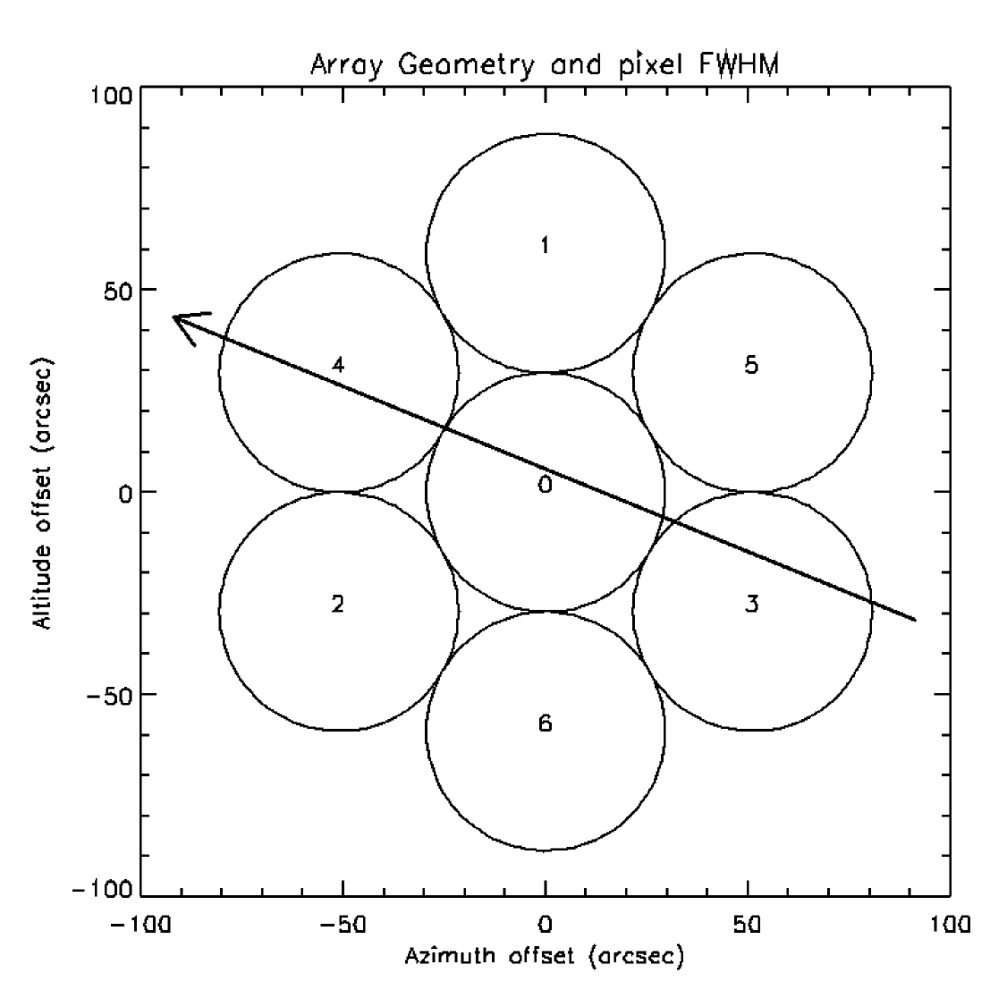
The simulated sky, typically generated by convolving a synthetic catalogue of extra-galactic sources with the telescope beam simulations , is assigned equatorial coordinates on the celestial sphere. The geometry of the array is defined and the beam positions on the sky are determined relative to the telescope bore-sight. The telescope is then arbitrarily located and the beams are scanned across the simulated sky model (in some pattern on an Alt-Az coordinate system for a given local time) and, using a rigorous calculation of the astrometry, the positional information and noiseless flux density time-series is determined for each bolometer in the array.

More realistic time-series are produced by incorporating features characteristic of real instruments, the pointing performance of the telescope, and the non-negligible contribution of the atmosphere (sky noise and attenuation).

Sources of instrumental noise in the time-series include: 1) addition of an uncorrelated Gaussian system noise component; 2) multiplication by gain factors (or different responsivities) for each detector; 3) addition of independent low frequency $1/f$ noise for each bolometer time-series to model the slowly-changing detector baselines in long duration scans; 4) convolution with an $e^{-t/\tau}$ impulse function to mimic the instantaneous response of the detectors. The instrumental noise components for a linear detector are summarized by the following expression for the response:

$$I_{measured}=G\times F+I_{dark}$$ (1)

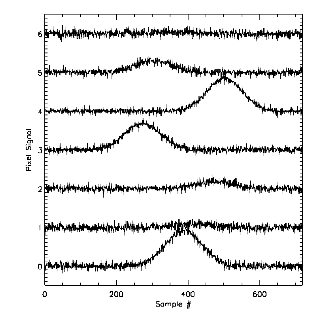
where $G$ is the detector gain, $F$ is the incident flux and $I_{dark}$ is the dark current consisting of both broad-band and $1/f$ noise components. The perfect astrometry may also be corrupted by adding random and systematic pointing errors. Fig. 1 shows the time-series for a 7-pixel feed-horn coupled array scanned across a point source at 500$\mu$m.

2 Sky Noise

Figure 2: A 360 $\times$ 180 degree² simulation of sub-mm sky emission at 850$\mu$m from cells of water vapour distributed in a flat plane at an altitude of 600m above the telescope.

Figure 3: Simulations of one-second point-and-stare total power observations with a fully-sampled (0.5-$F\lambda$) $40\times 40$ pixel monolithic array at 850$\mu$m with 14^′′ FWHM beams. In the case of perfect flat-fielding (left panel), two significant sources with a S/N of 25 and 12$\sigma$ are clearly observed against a typical sky-background gradient. In contrast, the fainter of the sources blends into the background noise when the gains of the bolometers are only known to a precision of $\sim 1\%$ (right panel).

Sky noise at sub-mm wavelengths is due to variable emission from cells of water vapour moving across the field-of-view of the telescope. This sky signal is significantly greater than the astronomical signal, and errors introduced through its imperfect subtraction lead to increased noise and artifacts in the reduced data. Thus, this important component of noise must be considered in all realistic simulations of ground-based observations.

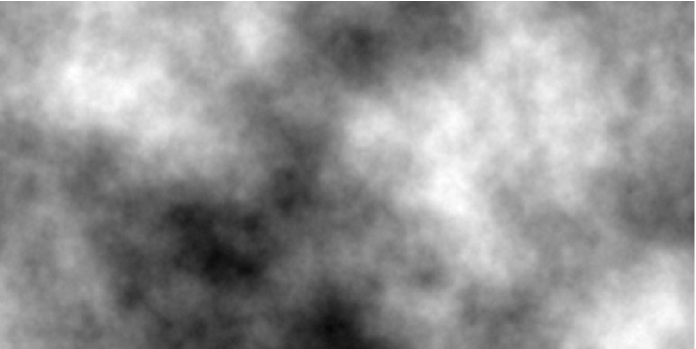
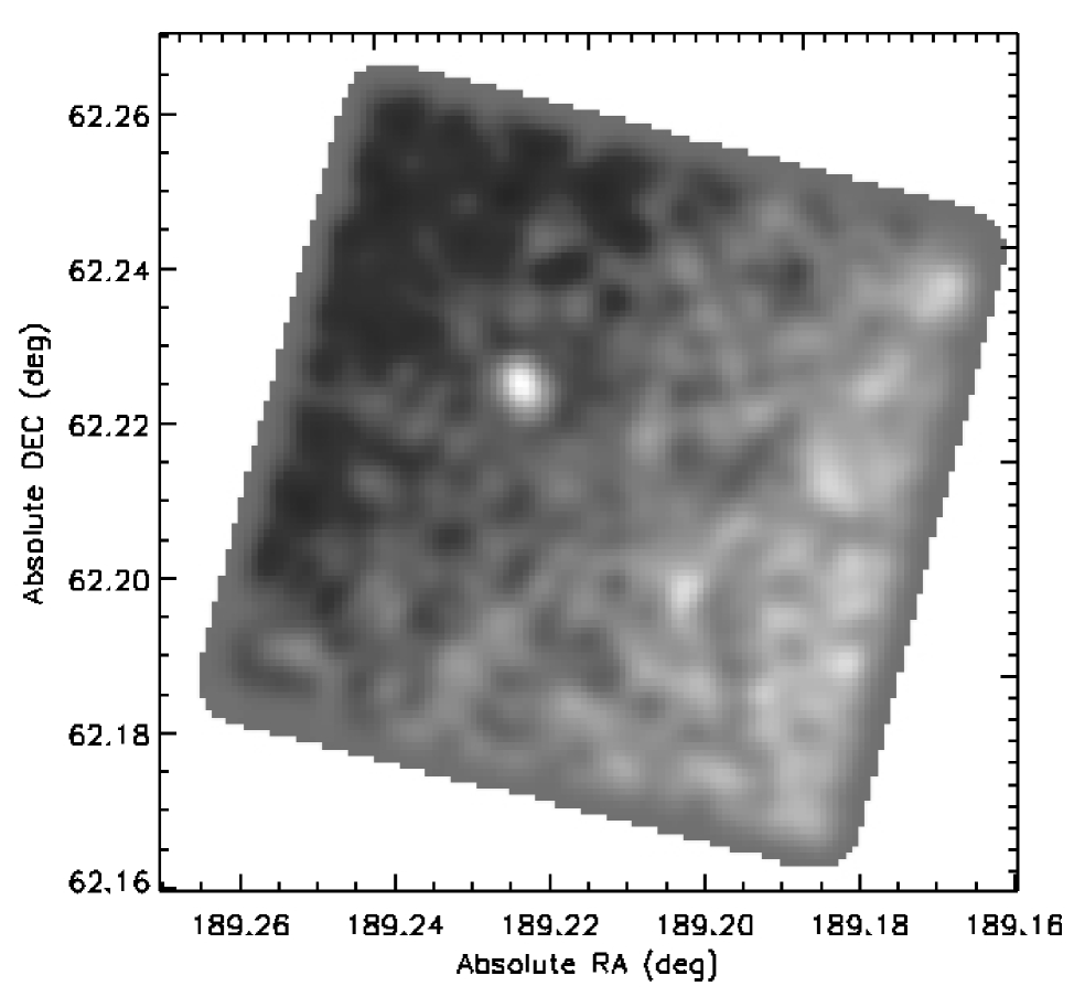
Data from the SCUBA camera scuba on the James Clerk Maxwell Telescope on Mauna Kea suggests the sky generates $1/f$-like noise that is correlated across the array. An empirical model that reproduces the observed spectrum of signals measured with the SCUBA array at 850$\mu$m assumes the sky consists of cells of water vapour, generated by convolving Gaussian noise with a symmetrical $(1/f)^{11/6}$ function, where $f$ is the 2-D spatial frequency, distributed in a flat-plane at some fiducial altitude, moving at the wind-speed above the telescope aperture (Fig. 2). This planar sky-model is passed across the simulated beams to produce a strong, variable sky signal.

Each 850$\mu$m pixel in the SCUBA2 array under good weather conditions will be illuminated by a sky background power of 8pW with a photon noise in a 1s integration of $4.3\times 10^{-5}$pW. While the total power of the sky may be removed by subtracting the median signal of the off-source sky bolometers, strong gradients still remain and can dominate the astronomical signals. DC sky measurements with SCUBA are used to estimate these gradients by transforming the time-series into a spatial signal via the recorded wind speed, assuming the emission is from a fixed altitude above the telescope, and scaling it accordingly for the different background loading of the SCUBA2 pixels. The estimated median change in the sky level across an 8 arcmin field of view is $7\times 10^{-4}$pW (about an order-of-magnitude greater than the photon noise). These estimates of the expected gradients and DC power levels allow the proper scaling and bias of the planar-cloud model used to generate the sky component of bolometer signals in the simulation.

Effective subtraction of the sky in the case of total power measurements depends critically upon the knowledge of detector gains and drifts. In Equation (1), $G$ and $I_{dark}$ vary from pixel to pixel and need to be removed using separate operations. The gain $G$ is slowing-changing, and characterized by performing flat-field observations with long integrations. The flat-fielding error must be smaller than the photon noise measured in the longest astronomical integration. In addition $G$ is multiplied by the large sky signal ($\gg$ astronomical signal), small errors in its measurement will lead to residual artifacts upon dividing it out of the response. An initial estimate suggests that $G$ will need to be measured to an accuracy of $\ll 1\%$. $I_{dark}$ consists of broad-band (white) noise plus a slowly varying $1/f$ component; the drift may be subtracted by measuring “dark” frames (1s integrations) in the absence of sky signal every few minutes.

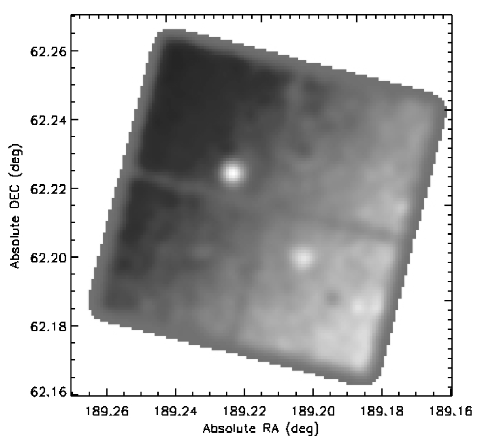
Fig. 3 demonstrates, for pointed total-power observations, two examples of the effects described above. In conclusion, the requirement to flat-field at sub-mm wavelengths with a precision of $\ll 1\%$ presents a major obstacle to the efficient use of large-format monolithic arrays on telescopes operated in total power mode.

References

- (1) Hughes, D. H. and Gaztañaga, E., “Submillimetre Galaxy Surveys” in Star Formation from the Small to the Large Scale, edited by F. Favata et al., ESLAB Symposium 33, Noordwijk, 2000, pp. 29–36, astro-ph/0004002.
- (2) Holland, W. S. et al., MNRAS, 303, 659–672 (1999).