Physical Implications of the X-ray Properties of Galaxy Groups and Clusters

Abstract

Within the standard framework of structure formation, where clusters and groups of galaxies are built up from the merging of smaller systems, the physical properties of the intracluster medium, such as the gas temperature and the total X-ray luminosity, are predicted to possess well defined self-similar scaling relations. Observed clusters and groups, however, show strong deviations from these predicted relations. We argue that these deviations are unlikely to be entirely due to observational biasses; we assume they are physically based, due to the presence of excess entropy in the intracluster medium in addition to that generated by accretion shocks during the formation of the cluster. Several mechanisms have been suggested as a means of generating this entropy. Focussing on those mechanisms that preheat the gas before it becomes a constituent of the virialized cluster environment, we present a simple, intuitive, physically motivated, analytic model that successfully captures the important physics associated with the accretion of high entropy gas onto group and cluster-scale systems. We use the model to derive the new relationships between the observable properties of clusters and groups of galaxies, as well as the evolution of these relations. These include the luminosity-temperature and luminosity-$\sigma$ relations, as well as the temperature distribution function and X-ray luminosity function. These properties are found to be a more accurate description of the observations than those predicted from the standard framework. Future observations that will further test the efficacy of the preheated gas scenario are also discussed.

1 Introduction

In currently favoured models for structure formation, virialized structures, such as groups and clusters of galaxies, are the results of sequences of gravitationally-driven accretion and mergers of smaller “building blocks”. According to the simplest (and what has effectively come to be regarded as the “standard”) of such models, the thermodynamic properties of the intracluster medium (ICM) are established by shocks and compression occuring during the accretion process. This model predicts that the intrinsic properties of the haloes (e.g.   mass, temperature, circular velocity, etc.) obey self-similar scalings. In turn, these imply that observable properties, such as the X-ray luminosity (L) and the temperature (T) of the intracluster gas in clusters and groups ought to scale as $L\propto T^{2}$ [Kaiser 1991, Eke et. al. 1996] and $L\propto T$ (Balogh, Babul & Patton 1999), respectively. Such predictions, however, do not match the observed relation for either the clusters, which is approximately $L\propto T^{3}$ [Edge, Stewart 1991, Markevitch 1998], or the groups, which is argued to be even steeper [Ponman et. al. 1996, Helsdon, Ponman 2000]. The theoretical models are also unable to account for the large, flat cores in the X-ray surface brightness profiles of the majority of the clusters [Lewis et. al. 2000]. Moreover, there is an indication of a discrepancy between the theoretical and the observed mass-temperature relationship. Several authors [Ettori, Fabian 1999, Nevalainen et. al. 2000, Xu, Jin, Wu 2001] have fit the mass-temperature data for systems with temperatures greater than 1 keV with a simple power-law and find $M\propto T^{1.7-1.9}$, which is steeper than the standard theoretical result: $M\propto T^{3/2}$. Finally, the standard model also predicts an entropy-temperature relationship that appears to be in conflict with the observed trend of a gradual flattening towards low temperatures [Ponman, Cannon, Navarro 1999, Lloyd-Davies, Ponman & Cannon 2000].

Broadly speaking, proposed resolutions to these problems can be grouped into three classes: those which appeal to observational biases or neglected physics such as cooling; those in which thermal energy is injected into the gas, either before or after collapse; and models which invoke non-thermal processes. We review these solutions in more detail below.

We start by addressing the possibility that no heating whatsoever is required. Firstly, it is possible that many, if not most, of the discrepant trends mentioned above are the result of observational biases arising due to the low surface brightnesses of the lower mass systems [Mulchaey 2000]; we will discuss this issue in §4. However, the best way to approach this problem is to create “mock” images from the models, and subject them to the same selection and reduction procedures as the real data (Poole et. al. , in preparation). Secondly, most of the analytic models of the ICM that we discuss below disregard the effects of cooling. Recent simulations, which include cooling (e.g. Lewis et. al. 2000; Pearce et. al. 2000; Muanwong et. al. 2001, Bryan & Voit 2001), have shown that this can have a significant effect on cluster and group gas profiles. One possibility is that as the low entropy gas in the central regions cools, condenses into dense, cold structures, and the higher entropy gas flows in to fill the volume, the X-ray luminosity will decrease. Whether this actually happens, however, has yet to be convincingly demonstrated. Lewis et. al. (2000) find that in their high resolution cluster simulations, the inclusion of cooling (and star formation) in fact leads to an increased X-ray luminosity. Finally, Bryan (2000) has suggested that galaxy formation is more efficient in groups than in clusters, which reduces the amount of hot gas and therefore the X-ray luminosity. However, this interpretation has been challenged by Balogh et. al. (2001), who claim that the observed trend on which Bryan’s conclusion is based is the result of biases in measuring the gas fractions of galaxy groups.

We now turn our attention to models which use energy injection to break the self-similar relations. Such a model was originally proposed by Kaiser (1991), and has been subsequently explored by many authors (e.g. Evrard & Henry 1991; Bower 1997; Cavaliere et. al. 1997, 1998; 1999; Balogh, Babul & Patton 1999; Wu, Fabian & Nulsen 2000; Lowenstein 2000; Tozzi & Norman 2001; Voit & Bryan 2001). In general, these models require that at least the central $\sim 10^{13}{\rm\,M_{\odot}}$ of the ICM has been injected with energy unassociated with the collapse and virialization of the groups and clusters at the level of 1–3 keV per particle.

There are many mechanisms for injecting the required energy into the intracluster medium. The one most commonly invoked is thermal energy from supernova explosions occuring within the group/cluster galaxies [Valageas, Silk 1999, Ponman, Cannon, Navarro 1999, Lowenstein 2000, Bower et al 2001, Brighenti, Mathews 2001]. The studies that have considered this possibility have, however, generally tended to conclude that even if the heating were to take place before collapse (when the energetics are most favourable), in order to have the required impact, the mean efficiency with which the supernovae energy is deposited into the ICM must be very high and that the initial mass function in the galaxies must be skewed towards high masses [Balogh, Babul, Patton 1999, Valageas, Silk 1999, Lowenstein 2000, Bower et al 2001, Brighenti, Mathews 2001]. The former is possible if a large fraction of the stars in the galaxies formed in intense starbursts [Heckman 2001] or, as suggested by recent high-resolution simulations by Lewis et. al. (2000), a significant fraction of the stars in the cluster are diffusely distributed within the intracluster volume. On the other hand, there is no compelling evidence for an IMF that is very different from that observed locally (e.g. Wyse 1997).

There is potentially another large source of thermal energy in quasars and active galactic nucleii (e.g. Valageas & Silk 1999; Wu et. al.  2000). Kormendy & Richstone (1995) and Magorrian et. al.  (1998) present strong evidence that most spheroidal galaxies are likely to harbour massive black holes of typical mass $\sim 10^{8}{\rm\,M_{\odot}}$ in their centers. When fueled, these black holes are expected to behave like quasars and under reasonable assumptions, there appears to be more than enough energy available from these objects to heat $\sim 10^{13}{\rm\,M_{\odot}}$ of gas in the surrounding environment to a temperature of $\sim 10^{6}$ K (e.g. Fabian 1999). Moreover, in order to account for the observed number density of quasars at $z\lower 2.15277pt\hbox{$\;\buildrel>\over{\sim}\;$}2$, Silk & Rees (1998) suggest that most of these black holes must have been active at some earlier epoch. The main drawback of this scheme is that the coupling between quasars and their surrounding medium is not well understood. One possibility is that the ambient medium is heated by shocks and turbulence created by fast moving jets produced by the active black holes (c.f. Kaiser & Alexander 1999; Rizza et al 2000). Another possibility is that quasars eject nearly spherical high velocity outflows that then shock-heats the ambient intergalactic medium. There is evidence for such outflows: Studies of the UV Broad Absorption Lines (BALs) suggest that these are created in outflows with velocities reaching $\sim 0.1c$ and having covering factors as large as 50% (e.g. Brandt et. al. 1999).

Yet another possible origin of pre-collapse heating is suggested by recent detailed high-resolution numerical studies of cluster formation in its proper cosmological setting [Lewis et. al. 2000] and of the evolution of the intergalactic medium [Cen et. al. 1995, Cen, Ostriker 1999, Davé et. al. 2001]. These simulations show that a significant fraction of the baryons outside virialized regions have temperatures in the range $10^{5}-10^{7}\;K$, at least at the present time, and that the corresponding entropy is comparable, if not somewhat greater, than the minimum entropy level required to explain the various X-ray correlations exhibited by groups and clusters. Cen et. al.  (1995) and Cen & Ostriker (1999) have suggested that this warm-hot diffuse medium is the result of the intergalactic medium being shocked during the formation of transient large-scale features such as sheets and filaments. A recent study by Davé et al (2001) of the distribution of the warm intergalactic medium supports this hypothesis. The implication of these results is that the entropy floor is a natural outcome of the currently favoured theoretical models.

Finally, the UV, radio and X-ray observations are increasingly showing that the intracluster medium is not a simple single-phase thermal medium as has been generally assumed but rather, is a rich, complex phenomenon, much like the interstellar medium. Specifically, there is growing evidence that the intracluster medium is composed of an X- ray luminous thermal component as well as a relativistic plasma — comprised of relativistic electrons, tangled magnetic fields and possibly even relativistic protons — ejected from quasars and active galactic nucleii (see, for example, Ensslin et. al. 1997). The presence of protons dramatically affects the evolution of the plasma and the extent to which it can affect the thermal component. Estimates of the energetics suggest that the total energy of such a plasma will be comparable to that of the thermal component (Ensslin & Kaiser 2000). Moreover, the presence of the protons ensures that the plasma will retain the bulk of its energy over cosmological timescales even though the electrons will radiate away their energy via synchotron/inverse-compton processes on very short timescales. The bubbles of relativistic plasma are expected to inflate until they reach pressure equilibrium with the ambient medium, in the process displacing the ambient thermal gas and creating low density cavities. There is growing evidence for the presence of such cavities in the X-ray observations of clusters [Bohringer et. al. 1995, Clarke et. al. 1997, McNamara et. al. 2000]. The detection of $\sim 5--10\;\mu$G magnetic fields via Faraday rotation measurements in over 16 clusters (Feretti et. al. 1995; 1999; Clarke, Kronberg, Bohringer 2001) lends further credence to the scenario. The presence of a relativisitic fluid with substantial pressure in the protogroup/protocluster environment will modify the accretion flow onto the haloes, especially those of lower mass. It will also affect the equilibrium distribution of gas in the haloes, resulting in lower gas densities in the central regions and hence, an “entropy floor”.

In this paper, we explore the consequences of entropy injection by one of the processes described above into the volume encompassing the intergalactic medium destined to form the ICM of groups and clusters. Drawing upon insights derived from detailed high resolution numerical simulations (e.g. Lewis et. al. 2000) as well as building on prior work by Balogh, Babul & Patton (1999), we have developed a simple, intuitive, physically motivated, analytic model that successfully captures most of the important physics associated with the accretion of high entropy gas onto the entire range of relevant halos, from low-mass groups to massive clusters.

A brief overview of the model is as follows: Unaffected by the energy injection, the dominant dark matter component will, in due course, collapse and virilize to form bound halos (§ 2.1). We assume that the dark matter in the halos will settle into a cuspy distribution as suggested by recent high-resolution numerical simulations. On the other hand, the collapse of the baryonic component is defined by the competition between gravity and the pressure forces engendered by the pre-heating (§ 2.2). If the maximum infall velocity purely due to the gravity of the halos ($\sim\sqrt{GM_{h}/R_{h}}$) is subsonic, the flow will be strongly modified by pressure and the gas will not experience accretion shocks. We assert that the baryons will accumulate onto such halos isentropically at the rate given by the adiabatic Bondi accretion rate. This element of our model was first described in Balogh, Babul, Patton (1999). The treatment presented there, however, was restricted to low mass halos because the “isentropic accretion” assumption is only valid for such systems. If the gravity of the halos is strong enough to drive the flow into the transonic or the supersonic regime, the gas will experience accretion shocks and the concomitant increase in entropy. In this paper, we extend our earlier model by taking our cue from recent high-resolution hydrodynamic simulations of clusters and modeling the entropy profile of the gas as $S(r)=S_{O}+\alpha\ln(r/r_{c})$ when the “isentropic accretion” assumption breaks down. Under all conditions, the distribution of hot diffuse gas inside the halos is governed by the requirement that it be in thermal pressure-supported hydrostatic equilibrium within the halo’s gravitational potential well.

The strength of our model lies in the fact it is both physically illuminating and allows us to compute and track the time-evolution of the X-ray properties of groups and clusters with relative ease. Our model neglects the complicated process of gas cooling but we note that, if the gas is preheated, gas cooling becomes less important because the gas density in low mass systems is reduced.

The present paper is organized as follows: In § 2, we briefly review the Balogh, Babul, Patton (1999) model and describe the extension to cluster scales, where accretion shocks become important. For specificity, we shall develop the model within the context of a flat $\Lambda$-CDM cosmological model with $\Omega_{\rm m}=0.3$, $h=0.75$ and unless otherwise specified, a big bang nucleosynthesis value $\Omega_{b}=0.019h^{-2}$ [Burles, Tytler 1998, Burles, Nollett, Turner 2001]. In § 3, we first present the gas distributions in our models, and the baryon fractions as a function of radius (§3.1). We then explore various scaling relations between gas temperature, lumionsity, and cluster mass or velocity dispersion, and make extensive comparisons with available data (§3.2–§3.4). We also present temperature/luminosity functions for objects spanning the entire mass range from groups to clusters, out to $z=1$, which demonstrate a very favourable comparison with the available data (§3.5). In § 4, we discuss the results in light of recent observations and critically assess the observational evidence favouring the “pre-heated model”. Our conclusions are summarized in § 5.

2 The Theoretical Framework

Our model for the formation of groups and clusters can be separated into two elements, which for simplicity’s sake we treat separately. The first element is the assemblage of the gravitationally bound structures (haloes) of the appropriate mass. This process is essentially driven by the collapse and virialization of the dark matter. The second element of the model involves the accumulation and the subsequent redistribution, within the halo, of the diffuse baryons.

2.1 The Dark Matter Haloes

Since dark matter is the gravitationally dominant component, we will assume that the first of the two processes mentioned above proceeds independently of the second. Specifically, we assume that the formation of the dark haloes as well as their internal structure and dynamics following virialization is everywhere dominated by the dark component.

Let us first consider a population of haloes of mass $M_{h}$ observed at redshift $z_{\rm obs}$. These haloes will have formed over a range of redshifts. This distribution of the redshift of formation of a population of haloes of a given mass can be derived using the analytic distribution function of Lacey, Cole (1993; 1994), assuming a spectrum of initial density fluctuations given by the Cold Dark Matter power spectrum [Bardeen et. al. 1986]. To do so, however, we need to specify what we mean by “formation”. Following Balogh, Babul, Patton (1999), we define the epoch of formation of a given halo as the redshift, $z_{\rm form}$, when 75% of the mass of the final halo mass at $z_{\rm obs}$ has been assembled and virialized in a halo. We note that throughout this paper, we will refer to the radius of this virialized region as the virial radius, ($R_{\rm vir}$), of the halo with the final (observed) mass $M_{h}$ that forms at redshift $z_{\rm form}$.

The remaining 25% of the halo’s final mass accumulates between redshifts $z_{\rm form}<z<z_{\rm obs}$. We assume that this additional mass accretes gently — so that internal structure of the halo is not disturbed — and that it largely accumulates in the outer regions of the halo. We will refer to the actual radius that encompasses mass $M_{h}$ at the epoch of observation ($z_{\rm obs}$) as $R_{h}$.

The above definition of halo formation is motivated by the results of numerical simulations [Navarro, Frenk, White 1996, Navarro, Frenk, White 1995] that suggest that the depth of the potential well, as traced by the circular velocity $V_{c}$ at the virial radius, remains relatively unchanged after $\sim$75% of the cluster mass is in place; the remaining 25% of the mass is accreted typically in minor mergers that do not significantly disrupt the mass distribution already in place.

Turning our attention to individual haloes, we assume that at ${z_{\rm form}}$ the distribution of the virialized mass is given by:

$$\rho_{DM}(r)={\rho_{DM,\circ}\left({r\over r_{s}}\right)^{-n}\left(1+{r\over r_{s}}\right)^{n-3}},$$ (1)

where $n=1.4$–$1.5$, $r_{s}$ is the scale radius and $\rho_{DM,\circ}$ is the normalization of the profile. Recent ultra-high resolution numerical simulations [Moore et. al. 1998, Klypin et. al. 1999, Lewis et. al. 2000] show that the radial distribution of dark matter in the haloes is best described by such a profile.

The normalization, $\rho_{DM,\circ}$, the size of the virialized region, $R_{\rm vir}$, and therefore, the shape and the depth of the gravitational potential well of the haloes will vary according to the epoch of halo formation; haloes of a given mass that form at an earlier epoch are denser, more compact and therefore, have a deeper potential. The normalization and the size of the virialized region at ${z_{\rm form}}$ ($R_{\rm vir}$) are specified by the requirements that (1) the mass contained within the virial radius is $M_{\rm form}=0.75M_{h}(z_{\rm obs})$ and (2) the mean density interior to $R_{\rm vir}$ satisfies the virialization criterion:

$$\bar{\rho}_{DM}(R_{\rm vir},z_{\rm form}) =\rho_{DM,\circ}(z_{\rm form})\left({3\over 3-n}\right)\left({r_{s}\over R_{\rm vir}}\right)^{n}\;\;\ \ \ \ \ \ \ \ \ \ \ \$$

$$\ \ \ \ \times\ _{2}F_{1}(3-n,3-n,4-n,-R_{\rm vir}/r_{s})$$

$$=F(z_{\rm form})^{2}\Delta_{c}(0)\rho_{\rm crit}(0),$$ (2)

where ${}_{2}F_{1}$ is the hypergeometric function and [c.f. Balogh, Babul, Patton (1999) for details]

$$F(z)^{2}= \left[1-\Omega_{m}+(1+z)^{3}\Omega_{m}\right]\Delta_{c}(z)/\Delta_{c}(0),$$

$$\Delta_{c}(z)= 49+96\Omega_{m}(z)+{200\Omega_{m}(z)\over 1+5\Omega_{m}(z)},$$

$$\Omega_{m}(z)= {\Omega_{m}(1+z)^{3}\over 1-\Omega_{m}+\Omega_{m}(1+z)^{3}}.$$

As for the scale radius, ultra-high resolution numerical simulations of cluster-scale haloes indicate that $r_{s}/R_{\rm vir}\approx 0.20$–0.25 [Lewis et. al. 2000]. We, therefore, assume $r_{s}=$0.25$R_{\rm vir}$. There are suggestions [Navarro, Frenk, White 1995, Bullock et al 2001] that this ratio may vary weakly with mass, with the ratio $r_{s}/R_{\rm vir}$ being somewhat smaller for lower mass systems. We have — for present purposes — chosen to ignore this complication. We do not expect the distribution of preheated gas in our model to be sensitive to the precise value of $r_{s}$ because the gas temperatures is much hotter than the “temperature” corresponding to the local gravitational potential.

2.2 The Hot Diffuse Gas in The Haloes

The fundamental assertion underlying our model is that one of the processes described in §1 injects energy into the volume encompassing matter destined to collapse to form groups and clusters of galaxies, raising the entropy of the diffuse gas in the volume such that $kTn_{e}^{-2/3}$ is in the range $100$–$500$ keV cm². For the present purposes, we shall assume that the added energy increases the thermal energy of the gas (as opposed to introducing a relativistic component). For simplicity, we also assume that there exists a single, universal, initial value of $kTn_{e}^{-2/3}$ and attempt to ascertain its value from the observations.

As described in Balogh, Babul, Patton (1999), the response of the heated diffuse gas to the gravitational collapse and virialization of the group/cluster dark matter halo is determined by the competition between the opposing forces of pressure and gravity. In the case of sufficiently small haloes, the pressure forces can slow down the gas accretion flow to the point where the flow is subsonic everywhere and these haloes will not be able to accrete their full complement of baryons, $M_{\rm b}=(\Omega_{\rm b}/\Omega_{\rm m})\;M_{h}$, by $z_{\rm obs}$. For such systems, we follow the prescription outlined in Balogh, Babul, Patton (1999). We assert that the gas distribution will accrete isentropically onto the haloes, and continue to evolve adiabatically. The equation of state of a gas distribution evolving thusly is $P=K_{\circ}\rho_{\rm gas}^{5/3}$, where the constant $K_{\circ}=kT/(\mu m_{H}\rho_{\rm gas}^{2/3})$ (where $\mu=0.59$ for fully ionized H and He plasma with Y=0.25) is a measure of the specific entropy of the gas and the accretion rate of the gas onto the halo is specified by the adiabatic Bondi accretion rate [Bondi 1952]:

$$\dot{M}_{\rm Bondi} =4\pi\lambda G^{2}M_{h}^{2}(\gamma K_{\circ})^{-3/2}\rho_{g}^{{3\over 2}(5/3-\gamma)},$$ (3)

$$\approx 1.86\pi\lambda G^{2}M_{h}^{2}K_{\circ}^{-3/2},\text{\ \ \ $\gamma=5/3$}$$

where $\lambda=0.25$ is the dimensionless accretion rate. For completeness, we note that we shall often quote $K_{\circ}$ in units of $K_{34}\equiv 10^{34}{\rm ergs}{\rm\,g}^{-5/3}{\rm\,cm}^{2}$, which, for a fully ionized H and He plasma with Y=0.25, is also equivalent to $kTn_{e}^{-2/3}=948.9{\rm\,keV}{\rm\,cm}^{2}$.

As discussed in Balogh, Babul, Patton (1999), the gas content of the halo at $z_{\rm obs}$ can be estimated as $M_{\rm gas}\approx\dot{M}_{\rm Bondi}t_{H}(z_{\rm obs})$, where $t_{H}$ is the Hubble time. Consequently, the halo gas fraction will scale as $M_{\rm gas}/M_{h}\propto M_{h}$. There is, however, a threshold mass above which the above estimate for $M_{\rm gas}$ implies $M_{\rm gas}/M_{h}>\Omega_{\rm b}/\Omega_{\rm m}$, i.e. a halo gas fraction that is larger than the universal baryon fraction. For such haloes, we cap the gas fraction at the universal value, recognizing that gas cannot fall in at a rate faster than that dictated by gravity. We also note that in this discussion of the halo gas fraction, we have implicitly assumed that the fraction of baryons locked up in stars is, to first order, negligible (e.g. Fukugita, Hogan, Peebles 1998, Balogh et. al. 2001) and therefore, $M_{\rm gas}\approx M_{\rm b}$.

In Balogh, Babul, Patton (1999), we determined the distribution of gas in the haloes by requiring that the isentropically accreted gas, with equation of state $P=K_{\circ}\rho_{\rm gas}^{5/3}$, is in thermal pressure-supported hydrostatic equilibrium within the halo’s gravitational potential well. This, combined with the total amount of gas in the haloes, completely specifies the gas density distribution in the haloes:

$$\begin{split}{\rho_{\rm gas}(r)\over\rho_{\rm gas}(R_{h})}&=\left[1+C\int_{r}^{R_{h}}\left({r^{\prime}\over R_{h}}\right)^{-2}M_{h}(r^{\prime})\;dr^{\prime}\right]^{3/2},\\ &\ \ \ \ \ \ C={2G\rho_{\rm gas}(R_{h})^{-2/3}\over 5K_{\circ}R_{h}^{2}}\end{split}$$ (4)

However, the above treatment, like the assertion that the gas will accrete onto the haloes isentropically breaks down for sufficiently high mass haloes. According to Equation 4, the density (and hence, the temperature) of the intracluster gas at the halo radius decreases with increasing halo mass, and tends towards zero. This result is clearly unphysical and indicative of the growing importance of accretion shocks.

Physically, the accretion flow is expected to behave as follows: during accretion onto a low mass halo, the gas velocity never exceeds the local sound speed and the flow can be treated as isentropic. However, as the mass of the halo is increased, the gas pressure forces become progressively less important in comparision with the gravity and the maximum infall velocity of the accreting gas will rise from subsonic through trans-sonic to supersonic. In the latter case, the gas that falls onto the halo will experience accretion shocks that will vary in strength from weak shocks, associated with mildly supersonic flows, to very strong shocks in the case of highly supersonic flows. Since the passage through shocks is marked by an increase in entropy, the flow can no longer be considered isentropic.

Taking our cue from the above physical description and the the results of recent high resolution hydrodynamic simulations of cluster formation [Lewis et. al. 2000], we model the distribution of gas in haloes where the gas has traversed through an accretion shock as follows: We demand that, regardless of how gas accretion occurs, the temperature of the intracluster at the halo radius at $z_{\rm obs}$ be greater than, or equal to, $\leavevmode\kern 1.00006pt\raise 2.58334pt\hbox{\sevenrm1}\kern-1.49994pt/\kern-1.99997pt\lower 3.01385pt\hbox{\sevenrm2}\;T_{h}$, where $kT_{h}\equiv\leavevmode\kern 1.00006pt\raise 2.58334pt\hbox{\sevenrm1}\kern-1.49994pt/\kern-1.99997pt\lower 3.01385pt\hbox{\sevenrm2}\;\mu m_{H}V_{c}^{2}(R_{h})$ is the temperature corresponding to the circular velocity at $R_{h}$.

The above constraint establishes a critical halo mass: $M_{\rm isen}$. For $M_{h}<M_{\rm isen}$, the isentropically accreted gas in hydrostatic equilibrium within the halo (with a density profile given by Equation 4) is, at $R=R_{h}$, hotter than $\leavevmode\kern 1.00006pt\raise 2.58334pt\hbox{\sevenrm1}\kern-1.49994pt/\kern-1.99997pt\lower 3.01385pt\hbox{\sevenrm2}\;T_{h}$. We can, therefore, safely assume that the gas accreted isentropically as described in Balogh, Babul, Patton (1999) and summarized above.

For more massive haloes, the temperature of the isentropic distribution of gas at $R_{h}$ is less than $\leavevmode\kern 1.00006pt\raise 2.58334pt\hbox{\sevenrm1}\kern-1.49994pt/\kern-1.99997pt\lower 3.01385pt\hbox{\sevenrm2}T_{h}$ and the gas must therefore be shock heated in order to meet our temperature constraint. To follow the shock history accurately requires a detailed treatment of the halo merger history, which we do not consider. However, at some early time, the most massive cluster progenitor will have had a mass less than $M_{\rm isen}$, and will have accreted its gas isentropically. We will assume, then, that a cluster is able to adiabatically accrete a total amount of gas given by $(\Omega_{\rm b}/\Omega_{\rm m})\;M_{\rm isen}$, and that this gas settles to the bottom of the potential well, forming an isentropic core with a radius $r_{c}$. Gas that accretes after the haloes have grown more massive than $M_{\rm isen}$ will be shocked (and shock-heated), with increasing strength as the halo grows more massive.

Let us consider a gas shell that accretes after the halo mass exceeds $M_{\rm isen}$ but before it has grown to its final (observed) mass $M_{h}(z_{\rm obs})$. As the gas shell is shocked, its entropy increases. Once through the shock, numerical simulation results [Lewis et. al. 2000] suggest that the gas shell will evolve adibatically within the halo potential, sinking deeper into the potential, compressing and heating up as additional gas shells are accreted. The gas in the shell will obey the relationship $P=K\rho_{\rm gas}^{5/3}$, where the value of $K$ is set by the post-shock value of the gas entropy in the shell.

Generalizing the above, we assume that even outside the isentropic core, the gas equation of state is $P=K(r)\rho_{\rm gas}^{5/3}$, where $K(r)=K_{\circ}$ for $r\leq r_{c}$. Again taking our cue from the Lewis et. al. (2000) simulation results, we model the entropy profile of the gas as

$$S(r)\equiv\ln\left({T/\rho_{\rm gas}^{2/3}}\right)=S_{\circ}+\alpha\ln(r/r_{c}),$$ (5)

where $\alpha=0$ for $r<r_{c}$, and therefore,

$$\ln K(r)=\ln K_{\circ}+\alpha\ln(r/r_{c}).$$ (6)

Neglecting the self-gravity of the gas and requiring that the gas is in thermal pressure-supported hydrostatic equilibrium within the halo potential yields:

$$\begin{split}\rho_{\rm gas}(r)&=\rho_{\rm gas}(r_{c})\left({r\over r_{c}}\right)^{-3\alpha/5}\ \ \ \ \ \ \ \ \ \ \ \ \ \ \ \\ &\;\;\times\left[1-C^{\prime}\int_{r_{c}}^{r}\left({r^{\prime}\over r_{c}}\right)^{-(2+3\alpha/5)}M_{h}(r^{\prime})\;dr^{\prime}\right]^{3/2}\!\!\!\!\!\!\!\!,\ \ \ \\ &\ \ \ \ \ \ \ \ \ \ \ \ C^{\prime}={2G\rho_{\rm gas}(r_{c})^{-2/3}\over 5K_{\circ}r_{c}^{2}}\end{split}$$ (7)

where, as noted above, $\alpha=0$ for $r<r_{c}$ and $M_{h}(r)$ is the halo dark matter mass within radius $r$. The gas temperature is given by:

$$kT(r)=\mu m_{H}K_{\circ}\left({r\over r_{c}}\right)^{\alpha}\rho_{\rm gas}(r)^{2/3}.$$ (8)

Specifying the three parameters: $r_{c}$, $\rho_{\rm gas}(r_{c})$ and $\alpha$ completely determines the model. The normalization, $\rho_{\rm gas}(r_{c})$, is determined by requiring that the total gas mass within $R_{h}$ is equal to $(\Omega_{\rm b}/\Omega_{\rm m})\;M_{h}$. The core radius is set by requiring $M_{\rm gas}(r_{c})=(\Omega_{\rm b}/\Omega_{\rm m})\;M_{\rm isen}$. Finally, the value of $\alpha$ is constrained by requiring that $T(R_{h})=\leavevmode\kern 1.00006pt\raise 2.58334pt\hbox{\sevenrm1}\kern-1.49994pt/\kern-1.99997pt\lower 3.01385pt\hbox{\sevenrm2}T_{h}$.

Figure 2: The three-dimensional radial profiles of the gas temperature, entropy and density for representative haloes at $z=0$, assuming that the entropy constant of the preheated gas is $K_{\circ}=0.45K_{\rm 34}$ or $kTn_{e}^{-2/3}\approx 427{\rm\,keV}{\rm\,cm}^{2}$. The thick, solid curves show the profiles for a halo with critical mass $M_{h}=M_{\rm isen}\equiv 8.4\times 10^{13}{\rm\,M_{\odot}}$, i.e. a halo where the gas is isentropic and its temperature at $R_{h}$ is equal to $\leavevmode\kern 1.00006pt\raise 2.58334pt\hbox{\sevenrm1}\kern-1.49994pt/\kern-1.99997pt\lower 3.01385pt\hbox{\sevenrm2}T_{h}$. The thin, solid lines show the profiles for a halo with subcritical mass ($M_{h}<M_{\rm isen}$). The dotted and the dashed lines correspond to the profiles in super-critical haloes of mass $M_{h}=4.75M_{\rm isen}=4\times 10^{14}{\rm\,M_{\odot}}$ and $M_{h}=47.5M_{\rm isen}=4\times 10^{15}{\rm\,M_{\odot}}$, respectively.

Figure 4: A different perpective on the three-dimensional radial profiles of the gas temperature, entropy and density for a group with $M_{h}=10^{13}{\rm\,M_{\odot}}$ (subcritical, dashed curves) and a cluster with $M_{h}=4\times 10^{14}{\rm\,M_{\odot}}$ (supercritical, solid curves). The thick lines correspond to the preheated model with $K_{\circ}=0.45K_{\rm 34}$ or $kTn_{e}^{-2/3}\approx 427{\rm\,keV}{\rm\,cm}^{2}$ and the thin lines show the standard, isothermal model with $T_{\rm gas}=T_{\rm vir}(z_{\rm form})$. The juxtaposition of the preheated and the isothermal profiles illustrates the impact of the entropy floor on the temperature and density profiles.

2.3 An isothermal model

To compare and contrast the properties of the model described above, we also construct a model in which the gas is assumed to be isothermal. We use the same halo potential, and again require the gas to be in pressure-supported hydrostatic equilibrium, but at a temperature $T=T_{\rm vir}(z_{\rm form})\approx T_{h}$.

3 Results

3.1 Properties of the Gas Distribution in Model Groups and Clusters

In Figures 2 and 4, we plot the three-dimensional radial profiles of the gas temperature, entropy and density for a set of representative haloes at $z=0$. In computing these, we have adopted a value of $K_{\circ}=0.45K_{\rm 34}$ or equivalently, $kTn_{e}^{-2/3}\approx 427{\rm\,keV}{\rm\,cm}^{2}$ (for a fully ionized H and He plasma with Y=0.25). This particular choice for the value of the entropy is the consequence of our requiring the model L–T relationship to match both the shape and the amplitude of the observed trend across the entire range of systems, from poor groups to rich clusters. We discuss this more fully in § 3.2, where we also compare our value to those adopted in other theoretical studies as well as to those derived from X-ray observations. We note that for our adopted entropy level, the corresponding value of the critical halo mass is $M_{\rm isen}=8.4\times 10^{13}{\rm\,M_{\odot}}$.

The temperature, entropy and density profiles for a subcritical halo with mass $M_{h}=3\times 10^{12}{\rm\,M_{\odot}}$ are plotted as the thin, solid curves in Figure 2. The gas has accreted onto the halo isentropically and therefore, the entropy profile is constant across the halo at a value of $kTn_{e}^{-2/3}\approx 427{\rm\,keV}{\rm\,cm}^{2}$. In addition, both the temperature and the density profiles are nearly flat, within a factor of two. We also note that the gas temperature at $R=R_{h}$ is nearly a factor of $\sim 4$ larger than $T_{h}$. As seen in Figure 4, the impact of the entropy floor is to push the temperature of the gas that accumulates in subcritical haloes well above the $T_{\rm vir}$ for the halo and, as a result, the gas is more diffuse and extended compared to that of the isothermal model.

As the halo mass is increased, the profiles tend to steepen. The profiles for a halo with critical mass $M_{h}=M_{\rm isen}=8.4\times 10^{13}{\rm\,M_{\odot}}$ are shown as thick, solid curves in Figure 2. This is the most massive cluster onto which the gas is able to accrete isentropically, hence the flat entropy profile. The temperature of the gas at $R=R_{h}$ is equal to $\leavevmode\kern 1.00006pt\raise 2.58334pt\hbox{\sevenrm1}\kern-1.49994pt/\kern-1.99997pt\lower 3.01385pt\hbox{\sevenrm2}T_{h}$. This is also true (by definition) of the temperature of the gas at $R=R_{h}$ in all haloes more massive than $M_{\rm isen}$. In Figure 2, the profiles of two super-critical haloes of mass $4\times 10^{14}{\rm\,M_{\odot}}$ and $4\times 10^{15}{\rm\,M_{\odot}}$ are shown as dotted and dashed curves, respectively. The gas in these two supercritical haloes, however, is not purely isentropic. Gas that accretes onto haloes that eventually grow to be supercritical while their mass is subcritical, will accrete isentropically and form the isentropic core. Gas that accretes onto these haloes after their mass has grown larger than $M_{\rm isen}$ will experience accretion shocks and an associated increase in entropy. An examination of the entropy profiles shows this core/envelope structure of the gas distribution in supercritical haloes. If, in these massive haloes, we characterize the size of the isentropic core by its radius $r_{c}$, then for a critical mass halo (short dashed curves), the core radius is equal to the radius of the halo and for supercritical haloes, $r_{c}<R_{h}$. We point out that the “kink” in the density and temperature profiles for super-critical haloes is a consequence of our treating the entropy profile as piecewise continuous. In reality, we expect this transition to be smooth.

For supercritical haloes, the impact of the entropy floor diminishes with increasing halo mass. This is best illustrated by a comparison of the preheated and isothermal profiles for a supercritical halo ($M_{h}=4\times 10^{14}{\rm\,M_{\odot}}$); we show this comparison in Figure 4. Beyond the central isentropic core, the temperature and density profiles of the two models are very similar. This is particularly true for the density profiles. The gentle decline in the temperature profile of the preheated model is, in fact, not due to preheating but rather due to compression of gas shells. This type of compressional heating is expected even if the gas had not been preheated. Recent cluster simulations also show a gently declining temperature profile towards the cluster periphery; in fact, outside the isentropic core, the temperature profile of the preheated gas model agrees very well with the results of the Lewis et. al.  (2000) simulation of a Virgo-mass cluster, which did not include any preheating. As an aside, we note that this latter result suggests that, strictly speaking, a purely isothermal model is not the most realistic standard with which to compare the pre-heated models, though it is still a fairly good approximation.

We note that one possible way of testing some of the key assumptions underlying our model, such as the universality of the value of the entropy floor, is to compare the radial density, temperature and entropy profiles of the gas distribution in our model halos against those of actual groups and clusters. Recent observations, based on ROSAT PSPC observations of low-temperature groups, suggest that entropy gradients in these groups are not flat (Lloyd-Davies, Ponman & Cannon 2000), in apparent conflict with the model presented here. However, the systematic uncertainties in determining even the projected temperature gradient from these data are sufficiently large that we cannot claim a strong discrepancy. Observational data from Chandra and XMM, which have superior spatial and energy resolution, will provide a stronger test. Furthermore, it is essential that the theoretical models be subjected to the same inherent observational biases due to low surface brightness, limited resolution and deprojection analyses, in order to make a fair comparison with the data (see § 4). We are currently in the process of carrying out analyses of this kind (Poole et al, in preparation)

Finally, for the convenience of readers who would like to reconstruct our model profiles for their own use, we plot in Figure 6, the values of the three model parameters, $\alpha$, $r_{c}$ and $\rho_{\rm gas}(r_{c})$, in haloes of different mass. We remind the reader that $\alpha$ determines the entropy profile for $r>r_{c}$; inside the core, the gas is isentropic and $\alpha=0$. Note that for clusters more massive than $M\approx 10^{14.5}{\rm\,M_{\odot}}$, the slope of the entropy profile outside the core is nearly independent of cluster mass (to within 10 per cent, $\alpha\approx 1.1$) while $r_{c}$ steadily decreases. This means that, outside the isentropic core, the entropy profiles of all clusters more massive than this limit are predicted to be nearly identical, once they are scaled to the value of the entropy at the virial radius.

Figure 6: A plot of the three model parameters, $\alpha$, $r_{c}$ and $\rho_{\rm gas}(r_{c})$, in haloes of different mass. $\alpha$ determines the entropy profile outside the core; inside the core, $\alpha=0$. These parameters correspond to an entropy floor of $K_{\circ}=0.45K_{\rm 34}$ or $kTn_{e}^{-2/3}\approx 427{\rm\,keV}{\rm\,cm}^{2}$.

Figure 8: The solid, short-dashed and long-dashed curves give the mean gas fraction within three different radii ($R_{h}$, $R_{200}$ and $R_{500}$, respectively) in the haloes at $z_{\rm obs}=0$, as a function of the total halo mass. The $R_{h}$ curve shows the gas fraction within the entire halo. This fraction is constrained to be no greater than $M_{\rm gas}/M_{h}=0.112$, the universal value for the cosmology under consideration. $R_{200}$ and $R_{500}$ are radii within which the mean dark matter mass density is 200 and 500 times the critical cosmological density at $z_{\rm obs}=0$, respectively. All of the curves are computed assuming that the entropy constant of the preheated gas is $K_{\circ}=0.45K_{\rm 34}$ or $kTn_{e}^{-2/3}\approx 427{\rm\,keV}{\rm\,cm}^{2}$.

In Figure 8, we plot the gas fraction $M_{\rm gas}/M_{h}$ within different regions characterized by $R_{h}$, $R_{200}$ and $R_{500}$ in the haloes at $z_{\rm obs}=0$, as a function of the total halo mass. These curves are computed using three dimensional gas and dark matter density profiles; the gas profile corresponds to that for an entropy constant $K_{\circ}=0.45K_{\rm 34}$. The short-dashed and long-dashed curves shows the gas fraction in regions within which the mean total mass density is 200 and 500 times the critical cosmological matter density at $z_{\rm obs}=0$, respectively. Although the amplitudes of the two curves are different, their behaviour is similar. For very low mass haloes ($M\lower 2.15277pt\hbox{$\;\buildrel<\over{\sim}\;$}7\times 10^{12}{\rm\,M_{\odot}}$), the gas fraction inside $R_{200}$ and $R_{500}$ is very small because the gas fraction in the entire halo is much less than the universal value of 0.0112 (c.f. the solid curve, which shows the gas fraction within the entire halo) and thermal pressure prevents the gas that is in the halo from concentrating in the center. With increasing halo mass, the halo gas fraction rises as $M_{\rm gas}/M_{h}\propto M_{h}$. The gas mass rises faster than the total halo mass. This increase, coupled with compression of the gas, results in a rise in the gas fractions within $R_{200}$ and $R_{500}$. As per our model, once the halo gas fraction reaches the universal value, it cannot increase any further, hence the flattening of the solid curve. From this point on, the increase in $M_{\rm gas}$ tracks the increase in $M_{h}$. The transition also impacts upon the growth of the gas fraction within $R_{200}$ and $R_{500}$. From this point on, the increase in the gas fraction within these two radii is entirely due to the compression and concentration of the gas. The increase is only checked when the mass enclosed within the radius under consideration exceeds $M_{\rm isen}$. For $R_{200}$, this happens at $M_{h}=1.3\times 10^{14}{\rm\,M_{\odot}}$ and for $R_{500}$, this happens at a slighly larger mass of $M_{h}=1.6\times 10^{14}{\rm\,M_{\odot}}$.

With an eye towards observations, the curves in Figure 8 predict that for systems with masses greater than $7\times 10^{12}{\rm\,M_{\odot}}$, there should be no observed variation in the gas fraction within the halo as a whole. However, the gas fraction within $R_{200}$ or $R_{500}$ should increase steadily with mass, approximately proportional to $M_{h}^{0.5}$ on mass scales below rich clusters. Recent analyses [David, Jones, Forman 1995, Mohr, Mathiesen, Evrard 1999, Fujita, Takahara 1999, Bryan 2000] suggest that the gas fraction in groups is lower that than in clusters, growing with halo mass as $M_{h}^{0.4}$; however, this trend has yet to be firmly established. As discussed by several authors (e.g. Mulchaey 2000; Roussel et. al. 2000; Balogh et. al. 2001), while many rich clusters have their X-ray emissions detected out to their peripheries, the detected X-ray emissions from groups is typically limited to the central regions. The lower gas fractions for groups, therefore, is more likely indicative of the paucity of gas in the central regions.

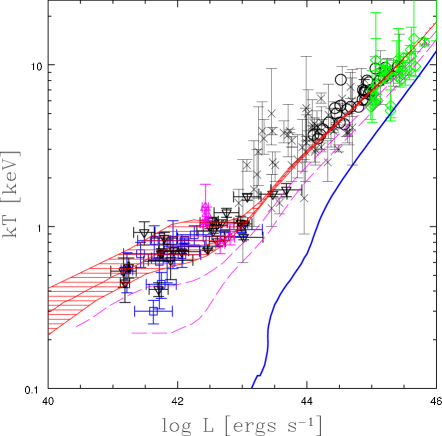
Figure 10: The $z=0$ luminosity–temperature relation, with data from Markevitch (1998, circles), Allen, Fabian (1998, diamonds), David et. al. (1993 ,crosses), Ponman et. al. (1996, squares), Mulchaey, Zabludoff (1998, triangles), and Helsdon, Ponman (2000, inverted triangles). The error bars are omitted from the Markevitch data, as they are smaller than the data symbols. The heavy, solid curve is the L–T relationship for haloes with isothermal gas at temperature $T=T_{\rm vir}(z_{\rm form})\approx T_{h}$, assuming the mean redshift of formation for haloes of a given mass. The hatched region shows the model results for an entropy constant of $K_{\circ}=0.45K_{\rm 34}$ or $kTn_{e}^{-2/3}\approx 427{\rm\,keV}{\rm\,cm}^{2}$. The width of the region reflects the range of formation redshifts for clusters of a given mass. Across the entire range, from poor groups to rich clusters, this “preheated” model results give an excellent match to observations. Finally, the two dashed curves show the model results for entropy constants $K_{\circ}=0.24K_{\rm 34}$ and $K_{\circ}=0.12K_{\rm 34}$ (i.e. $kTn_{e}^{-2/3}\approx 227{\rm\,keV}{\rm\,cm}^{2}$ and $kTn_{e}^{-2/3}\approx 114{\rm\,keV}{\rm\,cm}^{2}$, respectively).

3.2 The Luminosity-Temperature Relationship of Model Groups and Clusters

We use the latest version of the Raymond-Smith plasma code (Raymond, Cox, Smith 1976; Raymond, Smith 1977) to calculate the X-ray volume emissivity of the hot gas in the haloes. This code takes into account various radiative processes that can occur in low density plasma such as permitted, forbidden, and semiforbidden line transitions, dielectronic recombination, bremsstrahlung, radiative recombination, and two-photon continua. The code can treat plasma of arbitrary metallicity, taking into account the influence of elements up to Fe and Ni, with temperature ranging from $10^{4}$ K to $10^{8}$ K. This is important since the gas in the haloes of interest to us range from a few $\times 10^{6}$ K ($\sim 0.3{\rm\,keV}$) to $10^{8}$ K ($\sim 10{\rm\,keV}$). The X-ray emission of a plasma with $kT<4{\rm\,keV}$ is dominated by recombination radiation whereas emission of hotter gas is largely due to bremsstrahlung. For the purposes of calculating the X-ray emissivity of the hot plasma, we assume a constant metallicity of 0.3 Z_⊙.

In Figure 10, we plot the $z_{\rm obs}=0$ luminosity–temperature (L–T) relation for groups and clusters. The luminosity is the bolometric X–ray lumionsity of the halo and is computed by integrating the volume emissivity out to $R_{h}$, while the temperature is a luminosity–weighted average temperature (c.f. Equation 24 of Balogh, Babul, Patton 1999). We compare these results with data from from David et. al. (1993), Ponman et. al. (1996), Allen & Fabian (1998), Markevitch (1998), Mulchaey, Zabludoff (1998) and Helsdon & Ponman (2000). The Helsdon, Ponman luminosities have been corrected, using their published estimates for the correction factors, for emission between the observed radius and the virial radius. For the other group data, we have adopted an average correction (based on the Helsdon, Ponman analysis) of a factor of two in luminosity. We discuss this bias further in §4.

As a reference point, we show the results for the isothermal model as the heavy solid curve. This illustrates the now well-known result that the isothermal L–T curve is too steep to match the observations, even for clusters with temperatures greater than a few keV. In this temperature range, the relationship scales as $L\propto T^{2}$. Due to the dominance of recombination radiation at temperatures of less than 4 keV, the relationship steepens even more, approaching $L\propto T$. Also note that, in contrast with Balogh, Babul, Patton (1999), the isothermal model is overluminous at all temperatures. This is a consequence of adopting a dark matter potential which is very concentrated; in Balogh, Babul, Patton (1999), we assumed an isothermal potential with a flat core, which greatly reduces the total luminosity. We note further that haloes with $kT\mathrel{\hbox{\hbox to0.0pt{\hbox{\lower 4.0pt\hbox{$\sim$}}\hss}\hbox{$<$}}}0.5$ keV will radiate all of their energy in a Hubble time in the isothermal model, and, thus the approximation that cooling can be neglected breaks down severely in such systems.

Figure 10 also shows the L–T relationship for the preheated models with entropy constants $K_{\circ}=0.45K_{\rm 34}$ (the hatched region), $K_{\circ}=0.24K_{\rm 34}$ and $K_{\circ}=0.12K_{\rm 34}$ (the two dashed curves). A quick comparison of the three curves shows that the normalisation depends on the initial entropy. The lower of the two dashed curves is constructed with an entropy constant of $K_{\circ}=0.12K_{\rm 34}$ or $kTn_{e}^{-2/3}\approx 112{\rm\,keV}{\rm\,cm}^{2}$, close to that suggested by Helsdon, Ponman (2000) and Lloyd-Davies, Ponman, Cannon (2000). Although this curve may perhaps be seen to trace the lower envelope for the data, it is clear that it fails to match the majority of the observations across the entire range from poor groups to rich clusters.

To account for both the amplitude and the slope of the L-T relationships across the entire range from poor groups to rich clusters, we are required to consider models with entropy constants higher than $kTn_{e}^{-2/3}\approx 100{\rm\,keV}{\rm\,cm}^{2}$. The hatched region in Figure 10 corresponds to a model with $K_{\circ}=0.45K_{\rm 34}$ or $kTn_{e}^{-2/3}\approx 427{\rm\,keV}{\rm\,cm}^{2}$. This “preheated” model result gives an excellent match to observations across the entire range, from poor groups to rich clusters, and it is on the basis of this match to the observed L–T data that we adopt the $K_{\circ}=0.45K_{\rm 34}$ as our preferred model.

Our “preferred” value of the entropy floor is considerably higher than the value of $60$–$120{\rm\,keV}{\rm\,cm}^{2}$ (for $h=0.75$) derived by Lloyd-Davies et. al. (2000) from an analyses of ROSAT PSPC observations of low-temperature groups. As we have already noted (and elaborate upon further in § 4), comparing theoretical results with those derived from X-ray observations of groups is not straightforward due to the substantial systematic and statistical uncertainties in the observations resulting from the finite resolution of the X-ray telescopes and the intrinsic faintness of the groups. For one thing, only the very central regions of the systems are often detectable above the X-ray background (Mulchaey 2000; Roussel et. al. 2000; Helsdon, Ponman 2000) and typically, even this central region tends to be defined by only a small number of X-ray photons. As shown in Figure 11, even crudely modeling the limited X-ray extent reduces the required value of the entropy floor to $\approx 330{\rm\,keV}{\rm\,cm}^{2}$. However, even this latter value is still higher than the “observed value”. We, however, do not expect to be able to reduce the entropy floor significantly below this latter value without, for example, altering the dark matter profile of the halo and/or jettisoning the assumption that the value of the entropy floor is a universal constant. As illustrated in Figure 5, lowering the universal value of the entropy floor, while keeping the halo dark matter density distribution consistent with that seen in high-resolution cold dark matter simulations, leads to a drop in the amplitude of the model L–T curve and results in a mismatch between the theoretical and observational L–T correlations on the cluster scales. On these scales, the observational biases that affect the group results are not an issue. And neither are most of the key assumptions underlying our model, such as the “Bondi approximation”, as these predominantly affect only the distribution of gas in the low mass halos.

Comparing our value of the entropy floor with those required in other theoretical models, we note that Tozzi & Norman (2001) require a “high” level of entropy injection, in the range of $190$–$960{\rm\,keV}{\rm\,cm}^{2}$, to match the observed L–T correlations at $\sim 0.5$–$2{\rm\,keV}$. On the other hand, Cavaliere et. al.  (1999) assume an entropy injection that is comparable to the value measured by Lloyd-Davies et. al. (2000), and while their model L–T relationship is consistent with the observations on the group scale, as noted by Lloyd-Davies et. al. (2000), they fail to reproduce the slope of the L–T relationship at high temperatures. Finally, motivated by the results of Lloyd-Davies et. al. (2000), da Silva et. al. (2001) have recently carried out numerical simulations with a mean entropy floor of $\sim 80{\rm\,keV}{\rm\,cm}^{2}$ but they find that the $z=0$ groups and clusters in their simulation volume do not match the observed X-ray scaling relations. The upshot of all this is that there is considerable more work that needs to be done in order to bridge theory and observations. One possibility is that the entropy floor is a function of the halo mass (but see the discussion in the Appendix of Balogh, Babul & Patton 1999) and therefore, the value of the entropy floor on group scale is intrinsically lower than on the cluster scale. Alternatively, the results may be indicating that the underlying dark matter distribution is too cuspy. Flattening the inner profiles of the dark matter halos reduces the depth of the potential well and may result in the lowering of the entropy floor. (In Balogh, Babul & Patton 1999, we adopted dark matter halos with flat inner cores and required an entropy floor of $\sim 350{\rm\,keV}{\rm\,cm}^{2}$ as opposed to $\sim 430{\rm\,keV}{\rm\,cm}^{2}$ in the present study in order to match the observed group L-T results without even taking into account any observational biases.) Group and cluster data from Chandra and XMM, with superior spatial and energy resolution, are likely to go a long way towards resolving such issues.

The $K_{\circ}=0.45K_{\rm 34}$ model L–T curve is plotted in Figure 5 embedded within a hatched region, the width of which is related to the redshift range $z_{\rm obs}=0<z_{\rm form}<z_{1\sigma}$ within which 68.3% of the haloes have formed. This dispersion in the model L–T relation is also in excellent agreement with the observed scatter. The width of the hatched region is larger at low luminosities than at high luminosities, reflecting the broader distribution of formation times for low mass haloes [c.f. Balogh, Babul, Patton (1999), especially Figure 2, for details]. Interestingly, this 1-$\sigma$ band encompasses most of the group data shown in Figure 10. As noted by Balogh, Babul, Patton (1999), this match raises an extremely interesting possibility that the observed dispersion in the L–T relation is primarily due to the distribution of halo formation times. The model also predicts a very small dispersion at high luminosities and several studies [Fabian et. al. 1994, Arnaud, Evrard 1999, Markevitch 1998] have demonstrated that scatter in the L–T relation can be reduced to a very small value (an r.m.s. dispersion of about 0.11 in log L at a given T) by excluding cooling flow regions from the observed X-ray data. It is also worth pointing out that because of the very narow width of the hatched region at high luminosities, the $K_{\circ}=0.45K_{\rm 34}$ matches the observations in this regime.

At low temperatures and luminosities, the “preheated” model L–T relation scales as as $L\propto T^{4.7}$. This scaling is in excellent agreement with the results of Helsdon & Ponman (2000) based on their sample of 24 X-ray bright groups with temperatures ranging from $0.5$–$1.7{\rm\,keV}$. It is also consistent with the results of Mulchaey & Zabludoff (1998). The latter claim that their data is consistent with $L\propto T^{3}$ that describes the cluster data, which it is, but the sample consists of only nine groups spanning a rather narrow range in temperature.

At $L\approx 10^{42}{\rm ergs\,s^{-1}}$ ($T\approx 0.8{\rm\,keV}$), the L–T curve veers away from the low luminosity, low temperature asymptote. This point corresponds to the transition between haloes with $M_{\rm gas}/M_{h}<\Omega_{\rm b}/\Omega_{\rm m}$ and $M_{\rm gas}/M_{h}=\Omega_{\rm b}/\Omega_{\rm m}$. Prior to this transition point, the gas density and temperature gradients in the haloes are fairly shallow. Once past the transition point, the central gas density (and temperature) increases while that at the halo radius drops. The profiles, though steepening, are still sufficiently flat that the contribution of the hotter gas in the center to the emission-weighted temperature is offset by the cooler gas at larger radii, and the observed temperature remains roughly constant. In due course, however, the steeping of the gas density profiles with increasing halo mass begins to affect the emission-weighted temperature. As the gas profile steepens, an increasing fraction of the halo luminosity comes from the central regions where the gas is hotter and once a significant fraction of the luminosity originates in these central regions, the observed temperature begins to rise. Luminosity, on the other hand, depends sensitively on gas density and therefore, continues to increase throughout.

A second transition occurs at $L\approx 10^{43}{\rm ergs\,s^{-1}}$ ($T\approx 1{\rm\,keV}$). This transition separates systems onto which the gas accretes isentropically and systems in which accretions shocks become increasingly important. Shock heating imposes a lower limit to the gas temperature. As the halo mass grows larger and the shocked gas comes to dominate that intracluster medium, the L–T systems asymptotes to $L\propto T^{2.5}$, close to the observed $L\propto T^{2.7}$ relationship for clusters [Edge, Stewart 1991, Markevitch et. al. 1998].

Figure 12: The $z=0$ mass-temperature relation for the “preheated” model with entropy constant of $K_{\circ}=0.45K_{\rm 34}$ or $kTn_{e}^{-2/3}\approx 427{\rm\,keV}{\rm\,cm}^{2}$. The mass in the left panel is the total halo mass while in the right panel, it corresponds to the mass within $R_{500}$. The hatched region illustrates the dispersion expected due to the range for formation redshifts for groups and clusters of a given mass. Over the entire range, from very low to very high mass haloes, $M\propto T^{1.5-1.8}$, with the exact value of the power-law index depending on which mass is being considered. The short dashed curves show the $M\propto T^{3/2}$ relationship expected from self-similar scaling arguments. The self-similar model has been renormalized to match the pre-heated results in the $T\approx 2-3{\rm\,keV}$ range. For systems with $T<0.7{\rm\,keV}$, the normalization of the pre-heated model is nearly a factor of $\sim 3.5$ higher than the power-law extension of the high-temperature relationship. Nevalainen et. al. (2000) find that fitting the observed mass–temperature data for systems with temperatures greater than 1 keV with a simple power-law yields $M\propto T^{1.79}$ (long dashed line).

3.3 The Mass-Temperature Relationship

In Fig. 6, we plot the $z_{\rm obs}=0$ mass–temperature relation for groups and clusters for our preferred preheated model. The temperature plotted is, as before, the emission-weighted temperature, and the mass in the left plot is the total halo mass while in the right plot, it corresponds to the mass within $R_{500}$. A visual inspection of the figure shows that mass–temperature relationship is very sensitive to the thermal history of the gas.

For haloes with temperatures $T>1{\rm\,keV}$, the temperature rises monotonically with halo mass. The $\sim 1{\rm\,keV}$ scale separates systems onto which the gas accretes isentropically and systems in which accretion shocks become increasingly important. In the preheated model, the M–T relation for massive clusters is $M\propto T^{1.6-1.7}$, somewhat steeper than the self-similar result, if the mass being considered is the total mass, which is probably the best assumption for massive clusters (Mulchaey 2000). The slope is indistinguishible from the self-similar result if one scales against $M_{500}$. Ettori, Fabian (1999) as well as Nevalainen et. al. (2000) have fit the mass-temperature data for systems with temperatures greater than 1 keV with a simple power-law and find $M\propto T^{1.7-1.9}$, in reasonable agreement with the model.

For low temperature groups ($T<0.7{\rm\,keV}$), the preheated model predicts $M\propto T^{1.6}$, which is slightly steeper than the isothermal, self-similar $M\propto T^{3/2}$ relationship but similar to the M–T relation for massive pre-heated clusters. Note, however, that the emission-weighted gas temperature of a group of a given mass in the pre-heated model is nearly a factor of 3.5 higher than that expected from the extension of the cluster M–T relationship to lower masses.

As already discussed, in the preheated model the baryonic fraction of the low temperature groups is determined by the Bondi accretion rate and when this fraction exceeds the universal value, we argue that the baryon fraction of the halo will freeze at the universal value since gas cannot fall into the halo at a faster rate than that established by gravitationally induced accretion. As in the case of the L–T relation, this transition results in the model M–T curve breaking away from its low luminosity, low temperature asymptote at $T\approx 0.7{\rm\,keV}$. For a range of masses, the emission-weighted temperature of the gas is nearly independent of the halo mass. The reason for this behaviour has already been discussed in the context of the L–T relationship (Section 3.2).

3.4 The Luminosity-$\sigma$ Relationship

Since it is not possible to directly observe cluster masses, we consider the line-of-sight velocity dispersion for the model haloes. We define this as $\sigma_{\rm los}=V_{c}/\sqrt{2}$, which is a good approximation for haloes of our adopted potential [Lokas, Mamon 2001]. In Figure 14, we plot the $z_{\rm obs}=0$ $L$–$\sigma_{\rm los}$ relation for the groups and clusters. We also show variety of sources compiled from the literature: Mulchaey, Zabludoff (1998), David et. al. (1993), Ponman et. al. (1996), Markevitch et. al. (1998), and Xue, Wu (2000).

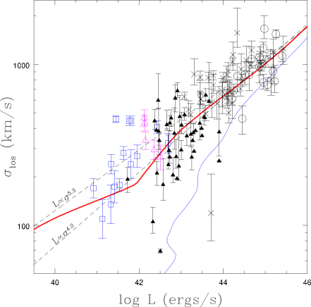
Figure 14: The thick solid curve shows the $z=0$ $L$–$\sigma_{\rm los}$ relation for the “preheated” model with entropy constant of $K_{\circ}=0.45K_{\rm 34}$ or $kTn_{e}^{-2/3}\approx 427{\rm\,keV}{\rm\,cm}^{2}$. We also show $L-\sigma_{\rm los}$ relation (thin solid curve) for the isothermal, self-similar model. The preheated model scales as $L\propto\sigma_{\rm los}^{5}$ at high luminosities, and $L\propto\sigma_{\rm los}^{9.4}$ at low luminosities. We also plot as dashed lines the power-law best-fit scaling found by Wu et. al. (1999, $L\propto\sigma_{\rm los}^{5.3}$) and Mulchaey, Zabludoff (1998, $L\propto\sigma_{\rm los}^{4.2}$). The data plotted are from Mulchaey, Zabludoff (1998, open triangles), David et. al. (1993, crosses), Ponman et. al. (1996, open squares), Markevitch et. al. (1998, circles), and Xue, Wu (2000, filled triangles).

The thick solid curve shows the $z=0$ $L$–$\sigma_{\rm los}$ relation for the “preheated” model with entropy constant of $K_{\circ}=0.45K_{\rm 34}$ or $kTn_{e}^{-2/3}\approx 427{\rm\,keV}{\rm\,cm}^{2}$. At high luminosities, the curve asymptotes to $L\propto\sigma_{\rm los}^{5}$ and at low luminosities, it scales as $L\propto\sigma_{\rm los}^{9.4}$. Given the considerable scatter in the data, the “preheated” model prediction is indistinguishable from the power-law scaling relations $L\propto\sigma_{\rm los}^{4.2}$, $L\propto\sigma_{\rm los}^{4.4}$, $L\propto\sigma_{\rm los}^{4.5}$, $L\propto\sigma_{\rm los}^{4.9}$ and $L\propto\sigma_{\rm los}^{5.3}$ of Mulchaey, Zabludoff (1998), Mahdavi & Geller (2001), Helsdon & Ponman (2000), Ponman et al (1996) and Wu et. al. (2000), respectively. In fact, analyses of the group and cluster data by Ponman et al (1996), Mulchaey, Zabludoff (1998), Helsdon, Ponman (2000) and Mahdavi, Geller (2001) all agree that as it stands, the $L$–$\sigma_{\rm los}$ relation for the groups is essentially the same as that for the clusters. As noted by Mulchaey (2000), “within the errors, the slopes derived by Mulchaey, Zabludoff(1998), Ponman et al (1996) and Helsdon, Ponman (2000) are indistinguishable.”

3.5 The Group-Cluster Temperature and Luminosity Function

The mass function of dark matter haloes is now quite well established by theory, and depends on cosmology and the shape of the power spectrum. Although Press-Schechter formalism, which has been used by many authors (including ourselves in Balogh, Babul, Patton 1999), provides a (surprisingly) good description of the mass function, large numerical simulations (e.g. Governato et. al. 1999) now provide us with a firm basis for the development of an improved formalism. We use the mass function of Jenkins et. al. (2001), which is a good, “universal” description, to within about 10%. We leave the normalisation, $\sigma_{8}$, as a free parameter.

The differential luminosity function is obtained from the mass function and the derivative $dM/dL$, which we evaluate numerically. An analagous procedure provides us with the differential temperature function; for comparison with observations, we integrate this function to give the cumulative temperature function, the number of galaxies with temperatures greater than $T$.

3.5.1 The Temperature Function

In Figure 16 we show the observed temperature function from Henry (2000), after making the necessary volume correction to convert the results to our adopted cosmological model. The solid points are the data at $z=0$. The open symbols represent clusters at $z\approx 0.4$, and show clear evidence for negative evolution; clusters of a given temperature are about three times less common at $z=0.4$ than they are locally.

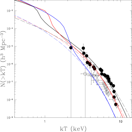
Figure 16: The cumulative temperature function. Data are from Henry (2000), converted to our cosmological parameters. The solid points are the $z=0$ data, and the open points are clusters at $z\approx 0.4$. The dashed lines are the isothermal models at $z=0$, $z=0.4$, and $z=1$, such that $N(>T)$ decreases with redshift at high temperatures. The solid lines are the preheated models at the same redshifts; the direction of evolution at the high temperature end is the same as for the isothermal models. We choose $\sigma_{8}=0.88$ and $\sigma_{8}=0.78$ for the isothermal and preheated models, respectively, to provide a good match to the $z=0$ data.

The isothermal model results are plotted as dashed lines in Figure 16. We have chosen $\sigma_{8}=0.88$ so that the model provides a reasonable match to the $z=0$ data. Model results at $z=0.4$ and $z=1.0$ are also plotted, and they demonstrate negative evolution for $kT>1$ keV. The direction and amount of evolution to $z=0.4$ in the data is well matched by the model.

The solid lines in Figure 16 represent the temperature function derived from our preheated models. In this case, we need to use a lower value of $\sigma_{8}=0.78$ to match the $z=0$ data. Thus, the normalisation of the power spectrum from the temperature function is dependent on the thermodynamic history of the gas, to about 10%. At high temperatures, $kT>3$ keV, the direction and amount of evolution of these models is quite similar to the isothermal models. Though the shape of the temperature function itself is steeper than that of the isothermal, it is not at the level which will be easily measured observationally. Therefore, apart from the normalisation, it is difficult to distinguish between the models on cluster scales.

At lower temperatures, the isothermal and preheated models diverge. At $z=0$, $N(>kT)$ rises sharply below $kT=1$ keV in the preheated model. This is due to the nearly flat relation between $T$ and $M$ as shown in Figure 12: halo masses between $10^{12.5}$ and $10^{14}$ at $z=0$ have nearly the same temperature of $kT=0.8$ keV. This is the mass range where the gas mass fraction is fixed at $\Omega_{b}/\Omega_{m}$, and $kT(R_{h})>{1\over 2}kT_{h}$, and we have discussed the cause of the constant temperature in this regime, in §3.2. The model therefore predicts an overabundance of clusters within a narrow temperature range around $kT=0.8$ keV, relative to the isothermal model. Below this temperature, the temperature function of the isothermal and preheated models become approximately parallel again, since the slopes of their respective $M-T$ relations are not very different. The direction of evolution of the temperature function below $kT=1$ keV also changes to positive evolution in the case of the preheated models. This is because the “constant temperature” regime occurs at a higher temperature at higher redshifts. Therefore, the sharp increase in the temperature function occurs at $kT=2$ keV at $z=1$, for example.

3.5.2 The Luminosity Function

The differential luminosity function is shown in Figure 18. The data are taken from the RDCS [Rosati, della Ceca, Norman, Giacconi 1998] and the EMSS [Gioia et. al. (1990), Henry et. al. 1992]. We correct the data to our chosen cosmology, and correct the luminosities to bolometric values. For the models, we use the values of $\sigma_{8}$ chosen to match the temperature function, namely $0.78$ for the preheated models, and $0.88$ for the isothermal models.

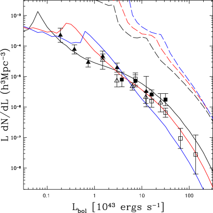
Figure 18: The differential luminosity function. Data are from the RDCS (triangles) and the EMSS (squares), converted to our cosmological parameters. Solid symbols are the low redshift data ($z<0.2$); the open symbols are high redshift clusters ($0.3<z<0.6$). The solid lines are the preheated models at $z=0$, $z=0.5$, and $z=1$, such that $N(>L)$ decreases with redshift at high luminosities. The dashed lines are isothermal models at the same redshifts; evolution is strictly positive in these models.

While the preheated model matches the $z=0$ data very well, the normalisation of the isothermal model is much too high. From the luminosity-temperature relation (Figure 10) it is clear that this should be so. For a given temperature, the isothermal luminosities are too high, even in the most massive clusters, where the gas is expected to be approximately isothermal. In particular, this is different from the result in Balogh, Babul, Patton (1999), where the isothermal luminosity function was not so discrepant with the data. The reason is that, in the model of Balogh, Babul, Patton (1999), we artificially introduced a flat core in the isothermal potential, to prevent the luminosities from diverging. As the size of this flat region is decreased, the luminosity of a given mass halo increases. In the current isothermal models there is no explicit need for such artificial structures since the potential we use does not lead to a divergent luminosity. However, the potential is necessarily steeper in the centre, which leads to higher densities and higher luminosities.

In the preheated models, the kink in the $z=0$ luminosity function at $10^{42}$ ergs s^-1 is due to a sharp change in slope of the $M-L$ relation, as shown in Figure 20. This corresponds to the point in the models where the gas mass fraction is equal to $\Omega_{b}/\Omega_{m}$, and there is a discontinuity in $dM/dL$. In the isothermal models, the non-monotonic shape at low luminosity is due to the corresponding very low temperatures (see Figure 10), where cooling is dominated by line emission and the cooling function changes rapidly with temperature. The shape of the luminosity function in this temperature regime will be quite sensitive to the metallicity, for that reason.

Figure 20: The relationship between mass and luminosity for the isothermal (dashed line) and preheated (solid line) models. The isothermal model is overluminous, relative to the preheated models, due to the steep central potential. This leads to the difference in luminosity functions seen in Figure 18.

The preheated model predicts mild negative evolution of the luminosity function at bright luminosities. This is in quite good agreement with the data, which show such evolution for $L>10^{44}$ ergs s^-1, but no evolution at lower luminosities. In contrast, the isothermal models show weak evolution at high luminosities, and stronger positive evolution at lower luminosities.

4 Discussion

There has been considerable interest in comparing and contrasting the correlations between the various X-ray properities, and between the X-ray and the optical properties, of groups and clusters. Although, at present there is no clear consensus on what the trends are indicating (Mulchaey 2000), studies of these kind can potentially provide considerable insight into the nature of the ICM in groups and clusters, and into the dominant mechanisms underlying their formation and evolution. While there is no doubt that to a fair extent the lack of consensus stems from the fact that the X-ray and optical properties of groups as not well determined — as discussed by Mulchaey (2000), the X-ray and optical properties of poor groups are subject to statistical and systematic uncertainties caused by small number statistics in both group members and X-ray photons — the fact that the discussions of the correlations have tended to focus on very different aspects also adds to the current state of affairs.

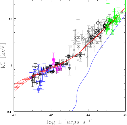
Figure 22: The $z=0$ luminosity–temperature relation for the preheated model (hatched region) and the isothermal model (solid line), in which the luminosity and temperature are computed by integrating the X-ray emissions out to the typical radius characterizing the spatial extent of the observed X-ray emissions from systems of a given temperature. The data are the same as in Figure 10; however the luminosities of the low temperature systems have not been corrected for emission outside the observed radius (since we now take account of this in the models). In constrast with the results presented in Figure 10, the entropy constant of the “preheated” model that best fits the data is $K_{\circ}=0.35K_{\rm 34}$ or $kTn_{e}^{-2/3}\approx 330{\rm\,keV}{\rm\,cm}^{2}$.

In an effort to help establish a common basis for discussing the commonalities and differences between the X-ray and optical properties of groups and clusters, we consider four questions:

1) Are the X-ray and optical trends of the clusters and groups accounted for by the standard isothermal model for their formation and evolution? Figures 10 and 14, for example, facilitate a comparison of the model predictions and the observed results. These figures clearly indicate that the isothermal model fails to account for the observations. However, there are both observational and theoretical caveats to consider. In computing the X-ray luminosities of our theoretical haloes, we integrated the emissivity over the entire halo and specifically, out to the virial radius in the plane of the sky. While the X-ray emission from rich clusters is indeed detected out to the cluster periphery, Mulchaey (2000), Roussel et. al. (2000) and [Helsdon, Ponman 2000] have pointed out that only the central regions of groups are detected, as the low surface brightness regions are overwhelmed by the X-ray background. Consequently, only a small fraction of the gas and thus, the X-ray luminosity, is directly detected in low temperature systems.

There are two strategies for working around the problem of differing X-ray extents of emissions from groups and clusters. One option is to attempt to correct the observations for the “missing flux”, in effect estimating the luminosity that would have been detected had the spatial extent of the observed X-ray emissions extended out to the virial radius in the plane of the sky, and then compare the corrected luminosity to theoretical results. This is the strategy that has been adopted, for example, by Mulchaey (2000) in the construction of his Figure 3 and by Helsdon and Ponman (2000). Such corrections, however, require either an assumption of a model for the properties and the spatial distribution of the gas outside the observed region or the adoption of some scheme (e.g.  the beta model) to extrapolate the distribution of the X-ray surface brightness distribution in groups out to their virial radii. Either approach is prone to gross systematic uncertainty. A better approach for carrying out “fair comparisons” between observations and theory is to subject the theoretical results to similar observational and instrumental biases and limitations as the observations. In essence, the goal is to create mock observations that are as realistic as possible and analyze these observations in exactly the same way as the real observations. We are in the process of carrying out a detailed analyses of this kind (Poole et al, in preparation) but, as a prelude, we have used the relationship between the observed temperature of a system and its projected radial extent of the detected X-ray emissions, derived from the observations and kindly provided to us by Mulchaey (2000, private communications), to construct theoretical luminosity-temperature curves that attempt to take into account, admittedly very crudely, the limited extent of detected X-ray emissions from low temperature systems. However, this has almost no effect on the isothermal models, as shown in Figure 22. This is because the temperature is fixed relative to the virial temperature and, furthermore, the steep density profiles mean that the luminosities are dominated by emission at $R<0.1R_{\rm vir}$. There is a larger effect on the preheated model, and a lower entropy constant of $K_{\circ}=0.35K_{\rm 34}$ or $kTn_{e}^{-2/3}\approx 330{\rm\,keV}{\rm\,cm}^{2}$ is required to fit the data. This is a factor of 0.78 smaller than in the “uncorrected” case. Comparing the original and truncated X-ray luminosities, we find a correction factor of $\sim 2$ for systems with $kT<1{\rm\,keV}$, which is in good agreement with the correction factors adopted by Helsdon and Ponman (2000) in their analyses. For hotter systems, the correction factor drops sharply to $\sim 1.3$ for systems with $kT\sim 2{\rm\,keV}$ and to $\sim 1.1$ by $kT=3{\rm\,keV}$. We note also that the dependence on formation epoch is greatly reduced in the low mass systems. While we recognize that our efforts to incorporate observational biases in the calculation of the theoretical curves are rather crude, the results do suggest that the isothermal model does not describe the gas distribution in groups or clusters.

2) Do the X-ray and optical correlations of groups an clusters scale similarly? This question is more difficult to address without actually going through the process of making mock but realistic observations of groups exhibiting similar correlations. We are in the process of doing so (Poole et. al. in preparation).

At the moment, given the large uncertainties in the measurements of group properties and the fact that the extent of the measured X-ray emissions from groups covers a small fraction of their projected surface area, Figures 10 and 14 do not rule out the possibility that the X-ray/optical correlations of groups and clusters scale in exactly the same way. The limited radial extent of the observations alone will cause departures from self-similar scaling on group scales resulting in steepening of the luminosity-temperature relationship (flattening in our Figure 10). Whether the observed steepening can be accounted for by this effect is the one of the central issues that has yet to be resolved.

However, even if cluster scaling relations provide a suitable description of the observations across the entire range, from rich clusters to groups, one is still faced with a puzzling conundrum: What is the theoretical basis for the scaling relations? What is the best model for describing the spatial, the dynamical and the thermodynamical state of the hot intracluster medium in the haloes? As discussed above, the isothermal model is certainly not it.

3) Is there then a theoretical model that can account for the observed trends of both groups and clusters? Based on the analyses presented in this paper, we would argue that the “preheated” model is just such a model. The “preheated” model appears to be able to account for most of the observed X-ray and optical correlations and the more careful analyses of the kind presently underway will allow us to further strengthen the model’s footing. In the process, we also expect that some of the details, such as the optimal range for model parameters including the entropy constant $K_{\circ}$, may change.

Much more importantly, there are some fundamental issues associated with the “preheating” model that have yet to be resolved: What is the cause of the preheating? Does preheating affect only limited volumes of the universe, volumes that eventually collapse to form groups and clusters, or is it ubiquitous? In the introduction, we briefly discussed some of these issues; however, there is considerably more work to be done.

Figure 24: Correlations between the integrated SZ flux and the X-ray luminosity for clusters and groups placed at z=0.1 (heavy curves) and z=1.0 light curves) for the preheated (solid) and isothermal (dashed) models.

4) Are there tests that one can subject the preheated model to? The preheated model has a clear signature in the density and entropy profiles, which can distinguish it from isothermal models. With the high sensitivity and good resolution of the Newton and Chandra telescopes, it is now possible to observe these profiles directly (e.g.  David et. al.  2001). However, to make this comparison between data and models fairly, it will be necessary to create realistic mock observations from the models and to “reduce” them in a way that is analagous with the real data, to properly account for effects such as spatial resolution, projection, and the limits of the energy bandpass (Poole et. al. , in preparation).

The Sunyaev-Zel’dovich (SZ) effect [Sunyaev, Zeldovich 1972, Sunyaev, Zeldovich 1980, Rephaeli 1995, Birkinshaw 1999] offers another potential probe of the thermal state of the intracluster medium in groups and clusters. Briefly, cosmic microwave background (CMB) photons passing through structures like galaxy clusters as they propagate towards us, will tend to get inverse Compton scattered by the hot electrons in the intracluster medium. While conserving the number of photons, the process does result in a preferential increase in the energy of the photons and hence, a distortion in the CMB spectrum in the direction of the structure.

Although long recognized as a potentially powerful tool with which to study the intra- as well as intercluster/intergalactic medium, SZ measurements have proven to be very difficult. Advances in detector technology, observing techniques, and the sheer perseverance of the people involved have, however, have brought the field to the threshold of maturity.

The study of the SZ distortion offers an independent means (from the studies of X-ray emissions) of probing the thermal state and the spatial distribution of intracluster gas in groups and clusters. In fact, SZ studies should prove to be particularly revealing since the SZ flux density of a cluster, integrated over its face, is proportional to the total thermal energy of the ICM [Bartlett 2000].

In recognition of the above, we are carrying out a detailed study of SZ effect as a test of the isentropic model and of the “preheating” scenario (McCarthy et. al. in preparation). As a prelude, we show in Figure 24, the plot of the ratio $S\nu/f\nu$ for groups and clusters, in units of mJy, against their X-ray luminosity. Here, $S\nu$ is the total SZ flux density from a cluster, found by integrating the surface brightness over the face of the group/cluster (c.f.  Bartlett 2000):

$$\begin{split}S_{\nu}&(x,M,z,z_{\rm form})=j_{\nu}(x)D_{a}^{-2}(z)\;\;\;\;\\ &\;\;\;\times\int{kT(M_{\rm form},z_{\rm form})\over m_{e}c^{2}}n_{e}(M_{\rm form},z_{\rm form})\sigma_{T}\;\;dV,\end{split}$$ (9)

where the integral is over the entire virial volume of the cluster, $D_{a}$ is the angular diameter distance, $\sigma_{T}=0.6652\times 10^{-24}$c m² is the Thompson cross section, and the function $j_{\nu}(x)$ describes the shape of the spectrum, as a function of the dimensionless frequency $x=h\nu/kT_{\circ}$. $T_{\circ}=2.78$ K is the temperature of the unperturbed CMB spectrum, and $j_{\nu}(x)=2(kT_{\circ})^{3}(hc)^{-2}f_{\nu}(x)$, with

$$f_{\nu}(x)={x^{4}\mbox{e}^{x}\over\left(\mbox{e}^{x}-1\right)^{2}}\left[{x\over\mbox{tanh}(x/2)}-4\right].$$ (10)

The plot also shows the predictions for the standard isothermal model.

Over four orders of magnitude in luminosity, the preheated model SZ flux scales almost exactly proportionally with luminosity. Even at high luminosities, the slope is very different from that of the isothermal model, and this difference increases toward lower luminosities. We can therefore expect to obtain interesting constraints from even the brightest SZ sources.

5 Summary

We have constructed a physical model for the gas distribution in dark matter haloes, assuming the gas has been preheated to a uniform but otherwise arbitrary entropy. Apart from this constraint, the critical assumptions are:

• Gas in virialised haloes is in pressure-supported hydrostatic equilibrium.

• Gas is accreted at the Bondi rate, up to the maximum that can be accreted gravitationally.

• Some fraction, between 0 and 1, of the gas is accreted adiabatically, and settles in the bottom of the potential to form an isentropic core. The size of this core is governed by a critical halo mass, below which we expect shocks to be negligible.

• Outside the isentropic core, the gas is shock heated. We assume a linear dependence of entropy on radius in this region, constrained to match the results of numerical simulations.

In addition to the detailed construction of the models, we have shown a variety of global scaling relations, between halo mass, velocity dispersion, and gas temperature and luminosity. We have made a detailed and critical comparison with data, and shown that the model is able to match the observed relations very well, over many orders of magnitude. The minimum entropy required is $K_{\circ}=0.45K_{\rm 34}$ or $kTn_{e}^{-2/3}\approx 427{\rm\,keV}{\rm\,cm}^{2}$. However, the strongest constraints on the models come from low-temperature systems like galaxy groups, and the observational biases in this data is troublesome enough that we anticipate the level of this entropy minimum is yet to be determined precisely.

References

- Arnaud, Evrard 1999 Arnaud, M., Evrard, A. E. 1999, MNRAS, 305, 631
- Allen & Fabian 1998 Allen, S. W., Fabian, A. C., 1998, MNRAS, 297, 57
- Balogh, Babul, Patton 1999 Balogh M.L., Babul A., Patton D.R., 1999, MNRAS, 307, 463
- Balogh et. al. 2001 Balogh, M. L., Pearce, F. R., Bower, R. G., Kay, S. T. 2001, MNRAS, 326, 1228
- Bardeen et. al. 1986 Bardeen J. M., Bond J. R., Kaiser N., Szalay A. S., 1986, ApJ, 304, 15
- Bartlett 2000 Bartlett J. G. 2000, astro-ph/0001267
- Birkinshaw 1999 Birkinshaw, M., 1999, Phys. Rep., 310, 98 ture, 380, 603
- Bondi 1952 Bondi H., 1952, MNRAS, 112, 195
- Bohringer et. al. 1995 Bohringer H., Nulsen P.E.J., Braun R., Fabian A.C., 1995 MNRAS, 274, 67
- Bower 1997 Bower R. G., 1997, MNRAS, 288, 355
- Bower et al 2001 Bower R.G., Benson A.J., Lacey C.G., Baugh C.M., Cole S., Frenk C.S., 2001, MNRAS, 325, 497
- Brandt et al 1999 Brandt W.N., Gallagher S.C., Laor A., Wills B.J., 1999, astro-ph/9910302, To appear in the Proceedings of the Bologna 1999 X-ray Conference “X-ray Astronomy 1999: Stellar Endpoints, AGN and the Diffuse Background”
- Brighenti, Mathews 2001 Brighenti, F., Mathews, W. G. 2001, ApJ 553, 103
- Bryan 2000 Bryan, G. L. 2000, ApJ, 544, L1
- Bryan, Voit 2001 Bryan, G. L., Voit, G. M. 2001, ApJ 556, 590
- Bullock et al 2001 Bullock, J. S., Kolatt, T. S., Sigad, Y., Somerville, R. S., Kravtsov, A. V., Klypin, A. A., Primack, J. R., Dekel, A. 2001, MNRAS, 321, 559
- Burles, Nollett, Turner 2001 Burles, S., Nollett, K. M., Turner, M. S., 2001, ApJ 552, 1
- Burles, Tytler 1998 Burles, S., Tytler, D. 1998, ApJ, 499, 699
- Cavaliere et. al. 1998 Cavaliere A., Menci N., Tozzi P., 1998, ApJ, 501, 493
- Cavaliere et. al. 1997 Cavaliere A., Menci N., Tozzi P., 1997, ApJ, 484, L21
- Cavaliere et. al. 1999 Cavaliere A., Menci N., Tozzi P., 1999, MNRAS, 308, 599
- Cen, Ostriker 1999 Cen, R., Ostriker, J. P., 1999, ApJ, 514, 1
- Cen et. al. 1995 Cen, R., Kang, H., Ostriker, J. P., Ryu, D., 1995, ApJ, 451, 436
- Clarke et. al. 1997 Clarke D.A., Harris D.E., Carilli C.L., 1997, MNRAS, 284, 981
- Clarke et. al. 2001 Clarke, T.E., Kronberg, P.P., Bohringer, H. 2001, ApJ, 547, L111
- da Silva et. al. 2001 da Silva, A.C. et. al. , 2001, ApJ, 561, 15
- Davé et. al. 2001 Davé, R., Cen, R., Ostriker, J. P., Bryan, G. L., Hernquist, L., Katz, N., Weinberg, D. H., Norman, M. L., O’Shea, B. 2001, ApJ 552, 473
- David, Jones, Forman 1995 David L. P., Jones C., Forman W., 1995 ApJ, 445, 578
- David et. al. 1993 David L. P., Slyz A., Jones C., Forman W., Vrtilek S. D., Arnaud K. A., 1993, ApJ, 412, 479
- David et. al. 2001 David L.P., Nulsen P.E.J., McNamara B.R., Forman W., Jones C., Ponman T., Robertson B., Wise M., 2001, ApJ, 557, 546
- Edge, Stewart 1991 Edge A. C., Stewart G. C., 1991, MNRAS, 252, 414
- Eke et. al. 1996 Eke V. R., Cole S., Frenk C. S., 1996, MNRAS, 282, 263
- Ensslin, Kaiser 2000 Ensslin, T.A., Kaiser, C.R., 2000 A&A, 360, 417
- Ensslin et. al. 1997 Ensslin, T.A., Biermann, P.L., Kronberg, P.P., Wu, X.-P. 1997, ApJ, 477, 560
- Evrard, Henry 1991 Evrard A. E., Henry J. P., 1991, ApJ, 383, 95
- Ettori, Fabian 1999 Ettori, S., Fabian, A.C. 1999, MNRAS, 305, 834
- Fabian 1999 Fabian A. C., 1999, MNRAS, 308, L39
- Fabian et. al. 1994 Fabian A. C., Crawford C. S., Edge A. C., Mushotzky R. F., 1994, MNRAS, 267, 779
- Feretti et. al. 1995 Feretti L., Dallacasa D., Giovannini G., Tagliani A., 1995, A&A, 302, 680
- Feretti et. al. 1999 Feretti L., Dallacasa D., Govoni F., Giovannini G., Taylor G.B., Klein U., 1999, A&A, 344, 472
- Fujita, Takahara 1999 Fujita, Y., Takahara, F. 1999, ApJL 519, 51
- Fukugita, Hogan, Peebles 1998 Fukugita, M., Hogan, C. J., Peebles, P. J. E. 1998, ApJ, 503, 518
- Gioia et. al. (1990) Gioia, I. M., Henry, J. P., Maccacaro, T., Morris, S. L., Stocke, J. T., Wolter, A. 1990, ApJ, 356, L35
- Governato et. al. 1999 Governato, F., Babul, A., Quinn, T., Tozzi, P., Baugh, C. M., Katz, N., Lake, G. 1999, MNRAS, 307, 949
- Heckman 2001 Heckman T.M., 2001, in Gas and Galaxy Evolution, ASP Conference Proceedings, Vol. 240. Edited by John E. Hibbard, Michael Rupen, and Jacqueline H. van Gorkom. San Francisco: Astronomical Society of the Pacific, p345 (astro-ph/0009075)
- Helsdon, Ponman 2000 Helsdon, S. F., Ponman, T. J., 2000, MNRAS, 315, 356
- Herny 2000 Henry J. P. 2000, ApJ 534, 565
- Henry et. al. 1992 Henry, J. P., Gioia, I. M., Maccacaro, T., Morris, S. L., Stocke, J. T., Wolter, A. 1992, ApJ, 386, 408
- Jenkins, A. et al., 2001 Jenkins, A. et al., 2001, MNRAS, 321, 372
- Kaiser, Alexander 1999 Kaiser C.R., Alexander P. 1999, MNRAS, 305, 707
- Kaiser 1991 Kaiser N., 1991, ApJ, 383, 104
- Klypin et. al. 1999 Klypin, A. A., Göttlober, S., Kravstov, A. V., Khokholov, A. M. 1999, ApJ, 516, 530
- Kormendy, Richstone 1995 Kormendy J., Richstone D.O., 1995, ARAA, 33, 581
- Lacey, Cole 1993 Lacey C., Cole S., 1993, MNRAS, 262, 627
- Lacey, Cole 1994 Lacey C., Cole S., 1994, MNRAS, 271, 676
- Lewis et. al. 2000 Lewis, G. F., Babul, A., Katz, N., Quinn, T., Hernquist, L., Weinberg, D. 2000 ApJ, 536, 623
- Lokas, Mamon 2001 Lokas, E. L., Mamon, G. A. 2001, MNRAS 321, 155
- Lowenstein 2000 Lowenstein M., 2000, ApJ, 532, 17
- Lloyd-Davies, Ponman & Cannon 2000 Lloyd-Davies, E.J., Ponman, T.J., Cannon, D.B. 2000, MNRAS, 315, 689
- Magorrian J. et. al. Magorrian J. et. al. , 1998, AJ, 115, 2285
- Mahdavi, Geller 2001 Mahdavi, A., Geller, M.J., 2001, ApJ, 554, L129
- Markevitch 1998 Markevitch M., 1998, ApJ, 504, 27
- Markevitch et. al. 1998 Markevitch M., Forman W. R., Sarazin, C. L., Vikhlinin A., 1998, ApJ 503, 72
- McNamara et. al. 2000 McNamara B.R. et. al. , 2000, ApJ, 534, L135
- Moore et. al. 1998 Moore, B., Governato, F., Quinn, T., Stadel, J., Lake, G. 1998, ApJ, 499, L5
- Mohr, Mathiesen, Evrard 1999 Mohr, J. J., Mathiesen, B., Evrard, A. E. 1999, ApJ, 517, 627
- Muanwong et. al. 2001 Muanwong, O., Thomas, P. A., Kay, S. T., Pearce, F. R., Couchman, H. M. P. 2001, ApJ 552, 27
- Mulchaey, Zabludoff 1998 Mulchaey J. S., Zabludoff A. I., 1998, ApJ, 496, 73
- Mulchaey 2000 Mulchaey, J. S. 2000, ARA&A, 38, 289
- Navarro, Frenk, White 1995 Navarro J. F., Frenk C. S., White S. D. M., 1995, MNRAS, 275, 720
- Navarro, Frenk, White 1996 Navarro J. F., Frenk C. S., White S. D. M., 1996, ApJ, 462, 563
- Nevalainen et. al. 2000 Nevalainen, J., Markevitch, M., Forman, W., 2000, ApJ, 532, 694
- Pearce et. al. 2000 Pearce, F. R., Thomas, P. A., Couchman, H. M. P., Edge, A. C. 2000, MNRAS, 317, 1029
- Ponman et. al. 1996 Ponman T. J., Bourner P. D. J., Ebeling H., Bohringer H., 1996, MNRAS, 283, 690
- Ponman, Cannon, Navarro 1999 Ponman, T. J., Cannon, D. B., Navarro, J. F. 1999, Nature, 397, 135
- Rephaeli 1995 Rephaeli, Y. 1995, ARA&A, 33, 541
- Raymond, Cox, Smith 1976 Raymond J. C., Cox D. P., Smith B. W., 1976, ApJ, 204, 290
- Raymond and Smith 1977 Raymond, J. C. and Smith, B. W. 1977, ApJ (Sup), 35, 419
- Roussel, Sadat, Blanchard 2000 Roussel, H., Sadat, R., Blanchard, A. 2000, A& A, 361, 429
- Rizza et al 2000 Rizza, E., Loken, C., Bliton, M., Roettiger, K., Burns, J. O., Owen, F. N., 2000 AJ, 119, 21
- Rosati, della Ceca, Norman, Giacconi 1998 Rosati, P., della Ceca, R., Norman, C., Giacconi, R. 1998, ApJ, 492, L21
- Silk, Rees 1998 Silk J., Rees M.J., 1998, A&A, 331, L4
- Sunyaev, Zeldovich 1972 Sunyaev, R. A., Zeldovich, Y. B. 1972, A&A, 20, 189
- Sunyaev, Zeldovich 1980 Sunyaev, R. A., Zeldovich, I. B. 1980, ARA&A, 18, 537
- Tozzi, Norman 2001 Tozzi, P., Norman, C. 2001, ApJ, 546, 63
- Valageas, Silk 1999 Valageas P., Silk, J., 1999, A&A, 350, 725
- Voit, Bryan 2001 Voit, G. M., Bryan, G. L. 2001, ApJ 551, 139
- Wu Xue Fang Wu X-P, Xue Y-J, Fang L-Z., 1999, ApJ, 524, 22
- Wu Fabian Nulsen 2000 Wu K.K.S., Fabian A.C., Nulsen P.E.J., 2000, MNRAS, 318, 889
- Wyse 1997 Wyse R.F.G., 1997, ApJ, 490, L69
- Xu, Jin, Wu 2001 Xu, H., Jin, G., Wu, X.-P. 2001, ApJ, 553, 78
- Xue Wu Xue Y, Wu X-P., 2000, ApJ, 538, 65