Formation of internal shock waves in bent jets

Abstract

We discuss the circumstances under which the bending of a jet can generate an internal shock wave. The analysis is carried out for relativistic and non–relativistic astrophysical jets. The calculations are done by the method of characteristics for the case of steady simple waves. This generalises the non–relativistic treatment first used by Icke (1991). We show that it is possible to obtain an upper limit to the bending angle of a jet in order not to create a shock wave at the end of the curvature. This limiting angle has a value of $\sim$75\text{\,}\mathrm{\SIUnitSymbolDegree}$$ for non–relativistic jets with a polytropic index $\kappa=4/3$, $\sim$135\text{\,}\mathrm{\SIUnitSymbolDegree}$$ for non–relativistic jets with $\kappa=5/3$ and $\sim$50\text{\,}\mathrm{\SIUnitSymbolDegree}$$ for relativistic jets with $\kappa=5/3$. We also discuss under which circumstances jets will form internal shock waves for smaller deflection angles.

1 Introduction

In a previous article (Mendoza & Longair, 2001), we discussed a mechanism by which galactic and extragalactic jets, can change their original straight trajectory if they pass through a stratified cold and high density region. For the case of galactic jets this could be a cloud in the vicinity of an H–H object. For extragalactic jets, this region could be a nearby galaxy, the interstellar medium of the host galaxy or the intracluster medium itself. Physically, what is important is that the medium interacting with the expanding jet from the source has a non–uniform density.

As mentioned by Icke (1991) and Mendoza & Longair (2001), when a jet bends, it is in direct contact with the surroundings and one should expect that entrainment from the surrounding gas might cause a severe disruption of the jet itself. Assuming that this entrainment is not important, for example by an efficient cooling, what its left is a high Mach number flow inside a collimated flow that bends. When a supersonic flow bends, the characteristics emanating at each point of the flow tend to intersect (Landau & Lifshitz, 1987; Courant & Friedrichs, 1976). Since every hydrodynamical quantity has a constant value on a given characteristic line, this intersection causes the different physical quantities in the flow, such as the density or pressure, to be multivalued. This situation cannot occur in nature and a shock wave is formed.

The formation of shock waves inside a jet are potentially dangerous. These shock waves could give rise to subsonic flow in the jet and collimation might no longer be achieved. The present article discusses the circumstances under which an internal shock wave should be expected in a bent jet. The analysis presented in this article generalises that made by Icke (1991) by introducing relativistic effects into the flow. This generalisation has a drastic effect on the results. Relativistic jets cannot bend as much as non–relativistic jets. As we will see below this occurs because, when relativistic effects are taken into account, the characteristic lines in the flow are beamed in the direction of the flow velocity. The beaming increases as the velocity of light is approached by the flow. In other words, the chances for an intersection between characteristic lines of uniform plane–parallel flow (before the bending) and a curved flow increase because of this beaming.

In order to analyse in detail the bending of relativistic jets we discuss the following points in each section. We write down the equations of relativistic hydrodynamics in section 2 and their non–relativistic counterparts. This sets the scene for discussing the propagation of disturbances in flows which leads naturally to the definition of the relativistic Mach number and characteristics. This generalises the traditional approach to gas dynamics and characteristic surfaces such as that discussed for non–relativistic hydrodynamics by Landau & Lifshitz (1987). The relativistic Mach number was first introduced by Chiu (1973) and some of its properties are well described by Königl (1980). The most important result to be proved in this section is the beaming of characteristic lines in the direction of motion of the flow for relativistic flows. Section 4 analyses the relativistic and non–relativistic cases for a flow depending on one angular variable, known as Prandtl–Meyer flow. This leads naturally to the generalisation of a type of flow called rarefaction waves in non–relativistic hydrodynamics (Landau & Lifshitz, 1987) which in turn is essential for the understanding of flows that move through a certain angle. In section 5 we use the main results of the Prandtl–Meyer flow to describe steady simple waves. These waves form naturally for steady plane parallel flow at infinity when the jet turns through an angle with a certain curved profile. It is then possible to apply the necessary physical ingredients to the steady simple waves formed. We then calculate an upper limit to the deflection of a jet in order to avoid the formation of a shock at the end of its curvature. This limit does not mean that a jet which curves through a small deflection angle is safe from generating an internal shock wave. So, we also calculate a lower limit, for which a shock could form at the onset of the curvature. Finally, in section 7 we discuss the astrophysical consequences of the results described above.

2 Basic equations

In order to understand the formation of internal shock waves in a bent jet it is necessary to understand some of the basic properties of the gas dynamics of relativistic flows.

The equations of motion for an ideal relativistic flow are described by the 4–dimensional Euler’s equation (Landau & Lifshitz, 1987):

$$\omega u^{k}\frac{\partial u_{i}}{\partial x^{k}}=\frac{\partial p}{\partial x^{i}}-u_{i}u^{k}\frac{\partial p}{\partial x^{k}},$$ (1)

in which Latin indices take the values $0,\ 1,\ 2,\ 3$. The vector $x^{k}=(\mathrm{\text{ $c_{0}$ }}t,\boldsymbol{r})$, where $\boldsymbol{r}$ represents the three dimensional radius vector, $c_{0}$ the speed of light and $t$ the time coordinate. The Galilean metric $g_{ik}$ for flat space time is given by $g_{00}\!=\!1$, $g_{11}\!=\!g_{22}\!=\!g_{33}\!=\!-1$ and $g_{ik}\!=\!0$ when $i\!\neq k\!$. The pressure is represented by $p$, $\omega=e+p$ is the enthalpy per unit proper volume and $e$ is the internal energy density. The four–velocity $u^{k}=\mathrm{d}x^{k}/\mathrm{d}s$ where the relativistic interval $\mathrm{d}s$ is given by $\mathrm{d}s^{2}=g_{kl}\mathrm{d}x^{k}\mathrm{d}x^{l}$. The values of the different thermodynamic quantities are measured in their local proper frame.

The space components of eq.(1) give the relativistic Euler equation:

$$\frac{\gamma\omega}{\mathrm{\text{ $c_{0}$ }}^{2}}\left\{\frac{\partial\boldsymbol{v}}{\partial t}+\boldsymbol{v}\cdot\boldsymbol{\mathrm{grad}}\,\boldsymbol{v}\right\}=-\boldsymbol{\mathrm{grad}}\,p-\frac{\boldsymbol{v}}{\mathrm{\text{ $c_{0}$ }}^{2}}\frac{\partial p}{\partial t},$$ (2)

where $\boldsymbol{v}$ is the three dimensional flow velocity and $\gamma$ is the Lorentz factor for a flow with this velocity.

For an ideal flow, in the absence of sources and sinks, the relativistic continuity equation is given by (Landau & Lifshitz, 1987):

$$\frac{\partial n^{k}}{\partial x^{k}}=0,$$ (3)

where the particle flux 4–vector $n^{k}\!=\!nu^{k}$ and the scalar $n$ is the proper number density of particles in the fluid.

A polytropic gas obeys the relation:

$$p\propto n^{\kappa},$$ (4)

where the polytropic index $\kappa$ is a constant and has the value $5/3$ for an adiabatic monoatomic gas in which relativistic effects are not taken into account. In the case of an ultrarelativistic photon gas it has a value of $4/3$. It is not difficult to show that for a polytropic gas, the speed of sound $a$ and the enthalpy per unit mass, the specific enthalpy, $w$ of are related to each other by the following formula (Stanyuokovich, 1960):

$$\frac{\mathrm{\text{ $c_{0}$ }}^{2}}{w}=1-\frac{1}{\kappa-1}\frac{a^{2}}{\mathrm{\text{ $c_{0}$ }}^{2}}.$$ (5)

The quantities in the relativistic case are defined with respect to the proper system of reference of the fluid, whereas in classical mechanics these quantities are referred to the laboratory frame. In the relativistic case the thermodynamic quantities, such as the internal energy density $e$, the entropy density $\sigma$ and the enthalpy density $\omega$ are all defined with respect to the proper volume of the fluid. In non–relativistic fluid dynamics, these quantities are defined in units of the mass of the fluid element they refer to. For instance, the specific internal energy $\epsilon$, the specific entropy $s$ and the specific enthalpy $w$ are all measured per unit mass in the laboratory frame. When taking the limit in which the speed of light $c$ tends to infinity we must also bear in mind that the internal energy density $e$ includes the rest energy density $nm\mathrm{\text{ $c_{0}$ }}^{2}$, where $m$ is the rest mass of the particular fluid element under consideration. Therefore the following non–relativistic limits should be taken in passing from relativistic to non–relativistic fluid dynamics:

$$mn \xrightarrow[\mathrm{\text{ $c_{0}$ }}\rightarrow\infty]{}\rho\sqrt{1-v^{2}/\mathrm{\text{ $c_{0}$ }}^{2}}\approx\rho\left(1-v^{2}/2c^{2}\right),$$

$$e \xrightarrow[\mathrm{\text{ $c_{0}$ }}\rightarrow\infty]{}nm\mathrm{\text{ $c_{0}$ }}^{2}+\rho\epsilon\approx\rho\mathrm{\text{ $c_{0}$ }}^{2}-\frac{1}{2}\rho v^{2}+\rho\epsilon,$$

$$\frac{\omega}{n} \xrightarrow[\mathrm{\text{ $c_{0}$ }}\rightarrow\infty]{}m\mathrm{\text{ $c_{0}$ }}^{2}+m\left(\epsilon+\frac{p}{\rho}\right)\approx m\left(\mathrm{\text{ $c_{0}$ }}^{2}+w\right),$$ (6)

where $\rho$ is the mass density of the fluid in the laboratory frame.

3 Characteristics and Mach number

The properties of subsonic and supersonic flow, are completely different in nature. To begin with, let us see how perturbations with small amplitudes are propagated along the flow for both subsonic and supersonic flows. For simplicity in the following discussion we consider two dimensional flow only. The relations obtained below are easily obtained for the general case of three dimensions.

If a gas in steady motion receives a small perturbation, this propagates through the gas with the velocity of sound relative to the flow itself. In another system of reference, the laboratory frame, in which the velocity of the flow is $v$ along the $x$ axis, the perturbation travels with an observed velocity $\boldsymbol{u}$ whose $x\text{ and }y$ components are given by:

$$u_{x}=\frac{a\cos\theta+v}{1+av\cos\theta/\mathrm{\text{ $c_{0}$ }}^{2}},$$ (7)

$$u_{y}=\frac{\gamma^{-1}a\sin\theta}{1+av\cos\theta/\mathrm{\text{ $c_{0}$ }}^{2}},$$ (8)

according to the rule for the addition of velocities in special relativity (Landau & Lifshitz, 1994). The polar angle $\theta$ and the velocity of sound $a$ are both measured in the proper frame of the fluid. Since a small disturbance in the flow moves with the velocity of sound in all directions, the parameter $\theta$ can have values $0\!\leq\!\theta\!\leq\!2\pi$. This is illustrated pictorially in Fig. 1.

\psfrag{F}{ $\theta$ }\psfrag{H}{ $\boldsymbol{v}$ }\psfrag{K}{ $a\hat{\boldsymbol{e}}_{r}^{\prime}$ }\psfrag{L}{ (a) }\psfrag{M}{ (b) }\psfrag{X}{ $\boldsymbol{v}$ }\psfrag{Y}{ $a\hat{\boldsymbol{e}}_{r}^{\prime}$ }\psfrag{Z}{ $\boldsymbol{u}$ }\psfrag{A}{ $\alpha$ }\psfrag{O}{ $0$ }\includegraphics[scale={0.50}]{fig.2.1.eps}

Figure 1: Region of influence of small amplitude perturbations. A perturbation of small amplitude is produced in the flow at some point $0$. This is carried by the flow which has velocity $\boldsymbol{v}$. In the case of subsonic flow, as shown in panel (a), the perturbation is able to propagate to the whole space. When the flow is supersonic the perturbation is propagated only downstream inside a cone with aperture angle $2\alpha$. The speed of sound $a$ and the angle $\theta$ are measured in a frame of reference in which the flow is at rest –the proper frame of the flow. The vector $\boldsymbol{u}$ is the relativistic addition of vectors $\boldsymbol{v}\text{ and }a\hat{\boldsymbol{e}}_{r}^{\prime}$, where $\hat{\boldsymbol{e}}_{r}^{\prime}$ is a unit radial vector in the proper frame of the flow.

Let us consider first the case in which the flow is subsonic, as illustrated in case (a) of Fig. 1. Since by definition $v\!<\!a$ and $\mathrm{\text{ $c_{0}$ }}^{2}>av$, it follows from eqs.(7)-(8) that $u_{x}(\theta\!=\!\pi)\!<\!0\text{ and }u_{y}(\theta\!=\!\pi)\!=\!0$. In other words, the region influenced by the perturbation contains the velocity vector $\boldsymbol{v}$. This means that the perturbation originating at $0$ is able to be transmitted to all parts of the flow.

When the velocity of the flow is supersonic, the situation is quite different, as shown in case (b) of Fig. 1. For this case, $u_{x}(\theta\!=\!\pi)\!>\!0\text{ and }u_{y}(\theta\!=\!\pi)\!=\!0$. In other words, the velocity vector $\boldsymbol{v}$ is not fully contained inside the region of influence produced by the perturbation. This implies that only a bounded region of space will be influenced by the perturbation originating at position $0$. For the case of steady flow, this region is evidently a cone. Thus, a disturbance arising at any point in supersonic flow is propagated only downstream inside a cone of aperture angle $2\alpha$. By definition, the angle $\alpha$ is such that it is the angle subtended by the unit radius vector $\hat{\boldsymbol{e}}_{r}$ with the velocity vector $\boldsymbol{v}$ at the point in which the azimuthal unit vector $\hat{\boldsymbol{e}}_{\alpha}$ is orthogonal with the tangent vector $\mathrm{d}(a\hat{\boldsymbol{e}}_{r}^{\prime})/\mathrm{d}\theta$ to the boundary of the region influenced by the perturbation. The unit vector $\hat{\boldsymbol{e}}_{r}^{\prime}$ is the unit radial vector in the proper frame of the flow. In other words, the angle $\alpha$ obeys the following mathematical relation:

$$\frac{\mathrm{d}\left(a\hat{\boldsymbol{e}}_{r}^{\prime}\right)}{\mathrm{d}\theta}\cdot\hat{\boldsymbol{e}}_{\alpha}=0.$$ (9)

Substitution of eqs.(7)-(8) into eq.(9) gives:

$$\tan\alpha=-\gamma\left\{\frac{1}{\tan\theta}+\frac{av}{\mathrm{\text{ $c_{0}$ }}^{2}\sin\theta}\right\}.$$ (10)

On the other hand, since $\tan\alpha\!=\!u_{y}/u_{x}$, it follows from eqs.(7)-(8) and eq.(10) that:

$$\tan\theta=-\frac{v}{a}\sqrt{1-\frac{a^{2}}{v^{2}}}\,,$$

and so eq.(10) gives a relation between the angle $\alpha$, the velocity of the flow $v$ and its sound speed $a$:

$$\tan\alpha=\gamma^{-1}\frac{a/v}{\sqrt{1-\left(a/v\right)^{2}}}$$ (11)

This variation of the angle $\alpha$ with the velocity of the flow is plotted in Fig. 2 for the case in which the gas is assumed to have a relativistic equation of state, that is, when $p\!=\!e/3$. The important feature to note from the plot is that the aperture angle of the cone of influence is reduced when the velocity of the flow approaches that of light.

From eq.(11) it follows that, as the velocity of the flow approaches that of light, the angle $\alpha$ vanishes. In other words, as the velocity reaches its maximum possible value, the perturbation is communicated to a very narrow region along the velocity of the flow.

In studies of supersonic motion in fluid mechanics it is very useful to introduce the dimensionless quantity $M$ defined as:

$$\frac{1}{M}\equiv\sin\alpha=\frac{\gamma_{a}}{\gamma}\frac{a}{v},$$ (12)

according to eq.(11). The quantity $\gamma_{a}\!=\!1/\sqrt{1-(a/\mathrm{\text{ $c_{0}$ }})^{2}}$ is the Lorentz factor calculated with the velocity of sound $a$. The number $M$ has the property that $M\!\rightarrow\!1\text{ as }v\!\rightarrow\!a\text{ and }M\!\rightarrow\!\infty\text{ as }v\!\rightarrow\!\mathrm{\text{ $c_{0}$ }}$. It also follows that $M\!>\!1$ if and only if $v\!>\!a$.

\psfrag{A}{ $2\alpha$ }\psfrag{B}{ $\boldsymbol{v}$ }\includegraphics[scale={0.78}]{fig.2.2.eps}

Figure 2: Region of influence of a perturbation for different values of the velocity of a relativistic gas with a sound speed $a\!=\!\mathrm{\text{ $c_{0}$ }}/\sqrt{*}{3}$. From left to right the closed loops correspond to values of the velocity $v$ of $0.0,\ 0.2,\ 0.4,\ldots,0.8$ in units of the speed of light $c_{0}$ . The perturbation is assumed to originate at the origin of the proper system of reference of the flow. In the case of supersonic flow, the region of influence occurs only downstream inside a cone with aperture angle $2\alpha$. This cone surrounds the corresponding loop and is tangent to it. When the flow is subsonic, the perturbation is transmitted to all the flow. As a particular example, the cone and the velocity vector have been drawn for the case in which the velocity is $v\!=\!0.8\mathrm{\text{ $c_{0}$ }}$.

The surface bounding the region reached by a disturbance starting from the origin $0$ is called a characteristic surface (Landau & Lifshitz, 1987). In the general case of arbitrary steady flow, the characteristic surface is no longer a cone. However, exactly as it was shown above, the characteristic surface cuts the streamlines at any point at the angle $\alpha$.

Let us briefly discuss the non–relativistic limit of the different physical circumstances presented above. To do this, we use the relations in eq.(6) with $\mathrm{\text{ $c_{0}$ }}\!\rightarrow\!\infty$ and, as usual for the non–relativistic case, we represent the speed of sound by $c$.

The dimensionless number $M$ satisfies the following relation:

$$\frac{1}{M}=\sin{\alpha}\xrightarrow[\mathrm{\text{ $c_{0}$ }}\rightarrow\infty]{}\frac{c}{v}$$ (13)

and is called in non–relativistic hydrodynamics the Mach number.

The results obtained concerning the relativistic and non–relativistic Mach number $M$ can be rewritten in the following way: the dimensionless Mach number $M$ increases without limits as the velocity of the flow takes its maximum possible value. This maximum value is the speed of light in the relativistic case and infinity in the non–relativistic one. The Mach number tends to zero as the velocity of the flow vanishes, and tends to unity as the velocity of the flow tends to the velocity of sound. The Mach number is greater than one for supersonic flow and less than unity when the velocity of the flow is subsonic in both, the relativistic and non–relativistic cases.

4 Prandtl–Meyer flow

Let us describe briefly the exact solution of the equations of hydrodynamics for plane steady flow which depends only on the angular variable $\phi$ only. This problem was first investigated by Prandtl and Meyer in 1908 (Landau & Lifshitz, 1987; Courant & Friedrichs, 1976) for the case in which relativistic effects were not taken into account. The full relativistic solution to the problem is due to Kolosnitsyn & Stanyukovich (1984).

For this case, Euler’s equation, eq.(1) and the continuity equation, eq.(3) can be written:

$$v_{\phi}=\frac{\mathrm{d}v_{r}}{\mathrm{d}\phi},$$ (14)

$$v_{r}n\gamma+\frac{\mathrm{d}\left(v_{\phi}n\gamma\right)}{\mathrm{d}\phi}=0,$$ (15)

$$\omega\gamma/n=\text{const},$$ (16)

where $v_{r}\text{ and }v_{\phi}$ are the components of the velocity in the radial and azimuthal directions respectively. Eq.(16) is the relativistic Bernoulli equation (Landau & Lifshitz, 1987) for this problem.

Using the definition of the speed of sound,

$$a=\mathrm{\text{ $c_{0}$ }}\left(\frac{\partial p}{\partial e}\right)_{\sigma}$$ (17)

in eq.(15) and eq.(16) it is found that:

$$v_{r}+\frac{\mathrm{d}v_{\phi}}{\mathrm{d}\phi}+v_{\phi}\left(1-\frac{a^{2}}{\mathrm{\text{ $c_{0}$ }}^{2}}\right)\frac{\mathrm{\text{ $c_{0}$ }}^{2}}{a^{2}}\frac{\mathrm{d}}{\mathrm{d}\phi}\ln\left(\omega/n\right)=0.$$ (18)

On the other hand, differentiation of $\gamma^{-2}$ with respect to the azimuthal angle $\phi$ and using eq.(16), gives:

$$v_{\phi}\left(v_{r}+\frac{\mathrm{d}v_{\phi}}{\mathrm{d}\phi}\right)+\mathrm{\text{ $c_{0}$ }}^{2}\left(1-\frac{v_{r}^{2}+v_{\phi}^{2}}{\mathrm{\text{ $c_{0}$ }}^{2}}\right)\frac{\mathrm{d}}{\mathrm{d}\phi}\ln\left(\omega/n\right)=0.$$ (19)

Multiplication of eq.(18) by $v_{\phi}$ and substracting this from eq.(19) gives:

$$v_{\phi}^{2}=a^{2}\left(1-\frac{v_{r}^{2}}{\mathrm{\text{ $c_{0}$ }}^{2}}\right).$$ (20)

Bernoulli’s equation, eq.(16), together with the value of the specific enthalpy for a polytropic gas given in eq.(5), can be rewritten

$$\left(1-\frac{v_{r}^{2}+v_{\phi}^{2}}{\mathrm{\text{ $c_{0}$ }}^{2}}\right)\left(1-\frac{1}{\kappa-1}\frac{a^{2}}{\mathrm{\text{ $c_{0}$ }}^{2}}\right)^{2}=\left(1-\frac{1}{\kappa-1}\frac{a_{0}^{2}}{\mathrm{\text{ $c_{0}$ }}^{2}}\right)^{2},$$ (21)

in which it has been assumed that at some definite point, the flow velocity vanishes and the speed of sound has a value $a_{0}$ there. It is always possible to make the velocity zero at a certain point by a suitable choice of the system of reference.

Eqs.(20)-(21) can be solved in terms of $v_{r}\text{ and }v_{\phi}$:

$$v_{r}^{2}/\mathrm{\text{ $c_{0}$ }}^{2}=1-F^{2}(a),$$ (22)

$$v_{\phi}^{2}=a^{2}F^{2}(a),$$ (23)

where

$$F^{2}(a)=\left(1-\frac{1}{\kappa-1}\frac{a_{0}^{2}}{\mathrm{\text{ $c_{0}$ }}^{2}}\right)^{2}\left(1-\frac{a^{2}}{\mathrm{\text{ $c_{0}$ }}^{2}}\right)^{-1}\left(1-\frac{1}{\kappa-1}\frac{a^{2}}{\mathrm{\text{ $c_{0}$ }}^{2}}\right)^{-2}.$$ (24)

Because $v_{r}\mathrm{d}v_{r}=\mathrm{\text{ $c_{0}$ }}^{2}F(a)F^{\prime}(a)\mathrm{d}a$, eq.(14) gives the required solution (Kolosnitsyn & Stanyukovich, 1984):

$$\phi+\phi_{0}=\pm\mathrm{\text{ $c_{0}$ }}\int{\frac{F^{\prime}(a)\mathrm{d}a}{a\sqrt{1-F^{2}(a)}}}.$$ (25)

This equation gives the speed of sound as a function of the azimuthal angle. From eqs.(22)-(23) it follows that the radial and azimuthal velocities can be obtained as a function of the same angle $\phi$. As a result, all the remaining hydrodynamical variables can be found. The sign in eq.(25) can be chosen to be negative by measuring the angle $\phi$ in the appropriate direction and we will do that in what follows.

Let us consider now the case of an ultrarelativistic gas and integrate eq.(25) by parts, to obtain:

$$\phi+\phi_{0}=\frac{\mathrm{\text{ $c_{0}$ }}}{a}\arccos F(a)+\mathrm{\text{ $c_{0}$ }}\int{\frac{\mathrm{d}a}{a^{2}}\arccos F(a)}.$$ (26)

For the case of an ultrarelativistic gas, the speed of sound $a$ is given by (Stanyuokovich, 1960) $a=\sqrt{\kappa-1}\ \mathrm{\text{ $c_{0}$ }}$ . In other words, this velocity is constant and so the integral in eq.(26) is a Lebesgue integral. Since this integral is taken over a bounded and measurable function over a set of measure zero, its value is zero.

Using eqs.(22)-(23) and eq.(26) the desired solution is obtained (Kolosnitsyn & Stanyukovich, 1984; Königl, 1980):

$$v_{r}=\mathrm{\text{ $c_{0}$ }}\sin\left\{\sqrt{\kappa-1}\left(\phi+\phi_{0}\right)\right\},$$ (27)

$$v_{\phi}=\sqrt{\kappa-1}\ \mathrm{\text{ $c_{0}$ }}\cos\left\{\sqrt{\kappa-1}\left(\phi+\phi_{0}\right)\right\},$$ (28)

for an ultrarelativistic equation of state of the gas.

For the non–relativistic case, in which $\mathrm{\text{ $c_{0}$ }}\!\rightarrow\!\infty$, eq.(25) gives for a polytropic gas with polytropic index $\kappa$:

$$\phi+\phi_{0}=-\sqrt{\frac{\kappa+1}{\kappa-1}}\int{\frac{\mathrm{d}\zeta}{\sqrt{1-\zeta^{2}}}},$$

where

$$\zeta\equiv\frac{a}{\mathrm{\text{ $c_{0}$ }}}\sqrt{\frac{\kappa+1}{\kappa-1}}\left\{1-\left(1-\frac{1}{\kappa-1}\frac{a_{0}^{2}}{\mathrm{\text{ $c_{0}$ }}^{2}}\right)^{2}\right\}^{-1/2},$$

and so, the required solution is (Kolosnitsyn & Stanyukovich, 1984):

$$\phi+\phi_{0}=\sqrt{\frac{\kappa+1}{\kappa-1}}\arccos\left(\frac{c}{c_{*}}\right),$$ (29)

where the speed of sound $a$ has been rewritten as $c$ to be consistent in the non–relativistic case. The critical velocity of sound $c_{*}$ is given by (Landau & Lifshitz, 1987):

$$c_{*}^{2}=\frac{2}{\kappa+1}c_{0}^{2}.$$ (30)

The value for the velocities can thus be calculated from eq.(14) and eq.(23) with $F(a)\!=\!1$:

$$v_{r}=\sqrt{\frac{\kappa+1}{\kappa-1}}c_{*}\sin\sqrt{\frac{\kappa-1}{\kappa+1}}\left(\phi-\phi_{0}\right),$$ (31)

$$v_{\phi}=c=c_{*}\cos\sqrt{\frac{\kappa-1}{\kappa+1}}\left(\phi-\phi_{0}\right).$$ (32)

Some important inequalities must be satisfied for the flow under consideration. First of all, eq.(25) together with eq.(5) and the first law of thermodynamics, $\mathrm{d}\left(\omega/n\right)=T\mathrm{d}\left(\sigma/n\right)+\left(1/n\right)\mathrm{d}p$ (Landau & Lifshitz, 1987), imply that $\mathrm{d}p/\mathrm{d}\phi\!<\!0$. Using this inequality and the fact that $\mathrm{d}e\!=\!\mathrm{\text{ $c_{0}$ }}^{2}\mathrm{d}p/a^{2}$ combined with the first law of thermodynamics, it follows that $\mathrm{d}n/\mathrm{d}\phi\!<\!0$. Also, using eqs.(22)-(23) it follows that $\mathrm{d}v/\mathrm{d}\phi\propto-\mathrm{d}a/\mathrm{d}\phi$ and necessarily $\mathrm{d}v/\mathrm{d}\phi\!>\!0$.

On the other hand, the angle $\chi$ that the velocity vector makes with some fixed axis is related to the velocity and the azimuthal angle $\phi$ by:

$$\chi=\phi+\arctan\left(v_{\phi}/v_{r}\right)$$ (33)

as it shown in Fig. 3. Thus, since the $\phi$ component of Euler’s equation, eq.(1) implies that:

$$\left(v_{r}+\frac{\partial v_{\phi}}{\partial\phi}\right)\frac{\gamma^{2}v_{\phi}\omega}{n}+\mathrm{\text{ $c_{0}$ }}^{2}\frac{\partial\left(\omega/n\right)}{\partial n}=0,$$

it follows that $\mathrm{d}\chi/\mathrm{d}\phi\!=\!-\left(v^{2}\gamma^{2}\omega/\mathrm{\text{ $c_{0}$ }}^{2}\right)^{-1}\mathrm{d}p/\mathrm{d}\phi$.

\psfrag{A}{ $v_{\phi}\hat{\boldsymbol{e}}_{\phi}$ }\psfrag{B}{ $\boldsymbol{v}$ }\psfrag{C}{ $v_{r}\hat{\boldsymbol{e}}_{r}$ }\psfrag{D}{ $\phi$ }\psfrag{E}{ $\chi$ }\psfrag{F}{ $0$ }\psfrag{G}{ $\alpha$ }\includegraphics[scale={0.83}]{fig.1.eps}

Figure 3: Relation between the velocity vector $\boldsymbol{v}\!=\!v_{r}\hat{\boldsymbol{e}}_{r}+v_{\phi}\hat{\boldsymbol{e}}_{\phi}$ and the angle $\chi$, as a function of the azimuthal angle $\phi$. $\chi$ is the angle that the velocity vector makes with certain fixed axis with origin O.

In other words, we have proved that for the flow with which we are concerned, the following inequalities are satisfied:

$$\mathrm{d}p/\mathrm{d}\phi<0,\quad\mathrm{d}n/\mathrm{d}\phi<0,\quad\mathrm{d}v/\mathrm{d}\phi>0,\quad\mathrm{d}\chi/\mathrm{d}\phi>0.$$ (34)

A flow with these properties is described as a rarefaction wave in non–relativistic fluid dynamics (Landau & Lifshitz, 1987) and we will use this name in what follows.

Another, very important property of this rarefaction wave is that the lines at constant $\phi$ intersect the streamlines at the Mach angle, that is, they are characteristics. Indeed, from Fig. 3, it follows that the angle $\alpha$ between the line $\phi\!=\!\textrm{const}$ and the velocity vector $\boldsymbol{v}$ is given by $\sin\alpha=v_{\phi}/v$. Using eqs.(22)-(24) it follows that this relation can be written as eq.(12). Because all quantities in the problem are functions of a single variable, the angle $\phi$, it follows that every hydrodynamical quantity is constant along the characteristics.

5 Steady simple waves

Let us now consider the two dimensional problem of steady plane parallel flow which then turns through an angle as it flows round a curved profile. A particular case of this problem, when the flow turns through an angle is described by Landau & Lifshitz (1987). For this particular situation the Prandtl-Meyer flow is obviously the solution and so, the hydrodynamical quantities depend on a single variable, the angle $\phi$ measured from a defined axis at the onset of the curvature. Because of this, all quantities can be expressed as functions of each other. Since this case is a particular solution to the general problem, it is natural to seek the solutions of the equations of motion in which the quantities $p,\ n,\ v_{x},\ v_{y}$ can be expressed as a function of each other. Evidently this imposes a restriction on the solution of the equations of motion since for two dimensional flow, any quantity depends on two coordinates, $x$ and $y$, and so any chosen hydrodynamical variable can be written as a function of any other two.

Because of the fact that the flow is uniform at infinity, where all quantities are constant, particularly the entropy, and because the flow is steady, the entropy is constant along a streamline. Thus, if there are no shock waves in the flow, the entropy remains constant along the whole trajectory of the flow and in what follows we will use this result.

In this case, Euler’s equation, eq.(2), and the continuity equation, eq.(3), are respectively:

$$v_{x}\frac{\partial v_{x}}{\partial x}+v_{y}\frac{\partial v_{x}}{\partial y}=-\frac{\mathrm{\text{ $c_{0}$ }}^{2}}{\gamma\omega}\frac{\partial p}{\partial x},$$

$$v_{x}\frac{\partial v_{y}}{\partial x}+v_{y}\frac{\partial v_{y}}{\partial y}=-\frac{\mathrm{\text{ $c_{0}$ }}^{2}}{\gamma\omega}\frac{\partial p}{\partial y},$$

$$\frac{\partial}{\partial x}\left(\gamma v_{x}n\right)+\frac{\partial}{\partial y}\left(\gamma v_{y}n\right)=0.$$

Rewriting these equations as Jacobians we obtain:

$$v_{x}\frac{\partial(v_{x},y)}{\partial(x,y)}-v_{y}\frac{\partial(v_{x},x)}{\partial(x,y)}=-\frac{\mathrm{\text{ $c_{0}$ }}^{2}}{\gamma\omega}\frac{\partial(p,y)}{\partial(x,y)},$$

$$v_{x}\frac{\partial(v_{y},y)}{\partial(x,y)}-v_{y}\frac{\partial(v_{y},x)}{\partial(x,y)}=+\frac{\mathrm{\text{ $c_{0}$ }}^{2}}{\gamma\omega}\frac{\partial(p,x)}{\partial(x,y)},$$

$$\frac{\partial(\gamma v_{x}n,y)}{\partial(x,y)}-\frac{\partial(\gamma v_{y}n,x)}{\partial(x,y)}=0.$$

We now take the coordinate $x$ and the pressure $p$ as independent variables. To make this transformation we have to multiply the previous set of equations by $\partial(x,y)/\partial(x,p)$. This multiplication leaves the equations the same, but with the substitution $\partial(x,y)\!\rightarrow\partial(x,p)$. Expanding this last relation and because all quantities are now functions of the pressure $p$ but not of $x$, it follows that:

$$\left(v_{y}-v_{x}\frac{\partial y}{\partial x}\right)\frac{\mathrm{d}v_{x}}{\mathrm{d}p}=\frac{\mathrm{\text{ $c_{0}$ }}^{2}}{\gamma\omega}\frac{\partial y}{\partial x},$$

$$\left(v_{y}-v_{x}\frac{\partial y}{\partial x}\right)\frac{\mathrm{d}v_{y}}{\mathrm{d}p}=-\frac{\mathrm{\text{ $c_{0}$ }}^{2}}{\gamma\omega}\frac{\partial y}{\partial x},$$

$$\left(v_{y}-v_{x}\frac{\partial y}{\partial x}\right)\frac{\mathrm{d}\left(\gamma n\right)}{\mathrm{d}p}+\gamma n\left\{\frac{\mathrm{d}v_{y}}{\mathrm{d}p}-\frac{\partial y}{\partial x}\frac{\mathrm{d}v_{x}}{\mathrm{d}p}\right\}=0.$$

Here we have taken $\partial y/\partial x$ to mean the derivative at constant pressure: $(\partial y/\partial x)_{p}$. Since every hydrodynamic quantity is assumed to be a function of the pressure, then in the previous set of equations it necessarily follows that $\partial y/\partial x$ is a function which depends only on the pressure, that is $(\partial y/\partial x)_{p}=f_{1}(p)$. Therefore:

$$y=xf_{1}(p)+f_{2}(p).$$ (35)

No further calculations are needed if we use the solution for the case in which a rarefaction wave is formed when flow turns through an angle (Landau & Lifshitz, 1987). This solution is given by the results of section 4. As was mentioned in that section, all hydrodynamical quantities are constant along the characteristic lines $\phi\!=\!\textrm{const}$. The particular solution of the flow past an angle obviously corresponds to the case in which $f_{2}(p)\!=\!0$ in eq.(35). The function $f_{1}(p)$ is determined from the equations obtained in section 4.

For a given constant value of the pressure $p$, eq.(35), gives a set of straight lines in the $x\text{--}y$ plane. These lines intersect the streamlines at the Mach angle. This occurs because the lines $y\!=\!xf_{1}(p)$ for the particular solution of the flow through an angle have this property. In other words, one family of characteristic surfaces correspond to a set of straight lines along which all quantities remain constant. However, for the general case, these lines are no longer concurrent.

The properties of the flow described above are analogous to the non–relativistic equivalent known as simple waves (Landau & Lifshitz, 1987). In what follows we will use this name to refer to such a flow.

\psfrag{B}{ $\alpha_{1}$ }\psfrag{C}{ $\phi_{1}$ }\psfrag{D}{ $\phi_{*}$ }\psfrag{E}{ $\phi_{*}-\phi$ }\psfrag{Z}{ $\theta$ }\includegraphics[scale={0.5}]{fig.2.eps}

Figure 4: Supersonic uniform flow at the left of the diagram bends around a curved profile OH. The Mach angle $\alpha_{1}$ is the angle made by the characteristics and the streamlines before the onset of the curvature. The characteristics make an angle $\phi_{1}$ with the “continuation” of the rarefaction wave formed at the onset of the curvature and the angle $\phi$ is measured from the line 0A’. The curvature causes the characteristic lines to intersect eventually and this occurs at point K in the diagram, giving rise to a shock wave represented as the segment KL.

Let us now construct the solution for a simple wave once the curved profile is fixed. Consider the profile as shown in Fig. 4. Plane parallel steady flow streams in from the left of point O and flows around the curved profile. Since we assume that the flow is supersonic, the effect of the curvature starting at O is communicated to the flow only downstream of the characteristic OA generated at point O. The characteristics to the left of OA, region 1, are all parallel and intersect the $x$ axis at the Mach angle $\alpha_{1}$ given by eq.(12):

$$\sin\alpha_{1}=\frac{\sqrt{1-\left(v_{1}/\mathrm{\text{ $c_{0}$ }}\right)^{2}}}{\sqrt{1-\left(a/\mathrm{\text{ $c_{0}$ }}\right)^{2}}}\ \frac{a}{v_{1}},$$ (36)

where the velocity $v_{1}$ is the velocity of the flow to the left of the characteristic OA. In eqs.(25)-(32) the angle $\phi$ of the characteristics is measured with respect to some straight line in the $x\text{--}y$ plane. As a result, we can choose for those equations the constant of integration $\phi_{0}\!\equiv 0\!$ . This means that the line from which the angle $\phi$ is measured has been chosen in a rather special way. In order to find the line which is the characteristic for $\phi\!=\!0$, let us proceed as follows. When $\phi\!=\!0$ and the gas is ultrarelativistic, eqs.(27)-(28) show that the velocity $v\!=\!a$ and for the non–relativistic case, it follows from eqs.(31)-(32) that the velocity takes the value $v\!=\!c$. In both cases this means that the line $\phi\!=\!0$ corresponds to the point at which the flow has reached the value of the local velocity of sound. This, however, is not possible since we are assuming that the flow is supersonic everywhere. Nevertheless, if the rarefaction wave is assumed to extend formally into the region to the left of OA, we can use these relations and then the characteristic line must correspond to a value of $\phi$ given by:

$$\phi_{1}=\sqrt{\frac{\kappa+1}{\kappa-1}}\arccos\left(\frac{c_{1}}{c_{*}}\right),$$ (37)

for a non–relativistic gas according to eq.(29), and

$$\phi_{1}=\frac{\mathrm{\text{ $c_{0}$ }}}{a}\arccos\frac{\sqrt{1-(v_{1}/\mathrm{\text{ $c_{0}$ }})^{2}}}{\sqrt{1-(a/\mathrm{\text{ $c_{0}$ }})^{2}}},$$ (38)

for the ultrarelativistic case according to eq.(21), eq.(24) and eq.(26). The angle between the characteristics and the $x$ axis is then given by: $\phi_{*}-\phi$, where $\phi_{*}\!=\alpha_{1}+\phi_{1},\text{ and the angle }\alpha_{1}$ is the Mach angle in region 1. The $x\text{ and }y$ velocity components in terms of the azimuthal angle $\theta$ are given by:

$$v_{x}=v\cos\theta,\qquad v_{y}=v\sin\theta,$$ (39)

and the values for the magnitude of the velocity, the angle $\theta$ and the pressure are given by:

$$v^{2}=c_{*}^{2}\left\{1+\frac{2}{\kappa-1}\sin^{2}\sqrt{\frac{\kappa-1}{\kappa+1}}\phi\right\},$$ (40)

$$\begin{split}\theta&=\phi_{*}-\phi-\alpha,\\ &=\phi_{*}-\phi-\arctan\left\{\sqrt{\frac{\kappa-1}{\kappa+1}}\cot\sqrt{\frac{\kappa-1}{\kappa+1}}\phi\right\},\\ \end{split}$$ (41)

$$p=p_{*}\cos^{2\kappa/\left(\kappa-1\right)}\sqrt{\frac{\kappa-1}{\kappa+1}}\phi,$$ (42)

for a non–relativistic gas according to eqs.(29)-(32) and using the fact that the Poisson adiabatic for a polytropic gas means that: $pc^{-2\kappa/\left(\kappa-1\right)}\!=\!\textrm{const}$. In the case of an ultrarelativistic gas, eqs.(26)-(28) together with Bernoulli’s equation and the fact that the enthalpy density $\omega\!=\!\kappa p/\left(\kappa-1\right)$ give:

$$v^{2}=\mathrm{\text{ $c_{0}$ }}^{2}\left\{1-\left(2-\kappa\right)\cos^{2}\sqrt{\kappa-1}\phi\right\},$$ (43)

$$\begin{split}\theta&=\phi_{*}-\phi-\alpha,\\ &=\phi_{*}-\phi-\arctan\left\{\sqrt{\kappa-1}\cot\sqrt{\kappa-1}\phi\right\},\\ \end{split}$$ (44)

$$p=p_{0}\left(2-\kappa\right)^{-\kappa/2\left(\kappa-1\right)}\cos^{-\kappa/\left(\kappa-1\right)}\sqrt{\kappa-1}\phi.$$ (45)

Since the angle $\phi_{*}-\phi$ is the angle between the characteristics and the $x$ axis, it follows that the line describing the characteristics is:

$$y=x\tan\left(\phi_{*}-\phi\right)+G(\phi).$$ (46)

The function $G(\phi)$ is obtained from the following arguments for a given profile of the curvature (Landau & Lifshitz, 1987). If the equation describing the shape of the profile is given by the points $X\text{ and }Y$ where $Y\!=\!Y(X)$, the velocity of the gas is tangential to this surface, and so:

$$\tan\theta=\frac{\mathrm{d}Y}{\mathrm{d}X}.$$ (47)

Now, the equation of the line through the point $(X,Y)$ which makes an angle $\phi_{*}-\phi$ with the $x$ axis is:

$$y-Y=\left(x-X\right)\tan\left(\phi_{*}-\phi\right).$$ (48)

Eq.(48) is the same as eq.(46) if we set:

$$G(\phi)=Y-X\tan(\phi_{*}-\phi).$$ (49)

If we start from a given profile $Y\!=\!Y(X)$ then, using eq.(47) we can find the parametric set of equations: $X\!=\!X(\theta)\text{ and }Y\!=\!Y(\theta)$. Substitution of $\theta\!=\!\theta(\phi)$ from eq.(41) or eq.(44) depending on whether the gas is non–relativistic or ultrarelativistic, we find $X\!=\!X(\phi)\text{ and }Y\!=\!Y(\phi)$. Substitution of this in eq.(49) gives the required function $G(\phi)$.

If the shape of the surface around which the gas flows is convex, the angle $\theta$ that the velocity vector makes with the $x$ axis decreases downstream. The angle $\phi-\phi_{*}$ between the characteristics leaving the surface and the $x$ axis also decreases monotonically. In other words, characteristics for this kind of flow do not intersect resulting in a continuous and rarefied flow.

On the other hand, if the shape of the surface is concave as shown in Fig. 4, the angle $\theta$ increases monotonically and so does the angle the characteristics make with the $x$ axis. This means that there must exist a region in the flow in which characteristics intersect. The value of the hydrodynamical quantities is constant for every characteristic line. This constant however changes for different non–parallel characteristics. In other words, at the point of intersection different hydrodynamical quantities, for example, the pressure, are multivalued. This situation cannot occur and results in the formation of a shock wave. This shock wave cannot be calculated from the above considerations, since they were based on the assumption that the flow had no discontinuities at all because the entropy was assumed to be constant. However, the point at which the shock wave starts, that is point K in Fig. 4, can be calculated from the following considerations. We can work out the inclination of the characteristics $\phi$ as a function of the coordinates $x\text{ and }y$. This function $\phi(x,y)$ becomes multivalued when these coordinates exceed certain fixed values, say $x_{0}\text{ and }y_{0}$. At a fixed $x\!=\!x_{0}$ the curve giving the value of $\phi$ as a function of $y$ becomes multivalued. That is, the derivative $\left(\partial\phi/\partial y\right)_{x}\!=\!\infty$, or $\left(\partial y/\partial\phi\right)_{x}\!=\!0$. It is evident that at the point $y\!=\!y_{0}$ the curve $\phi(y)$ must lie in both sides of the vertical tangent, else the function $\phi(y)$ would already be multivalued. This means that the point $(x_{0},y_{0})$ cannot be a maximum, or a minimum of the function $\phi(y)$ but it has to be an inflection point. In other words, the coordinates of point K in Fig. 4 can be calculated from the set of equations (Landau & Lifshitz, 1987):

$$\left(\frac{\partial y}{\partial\phi}\right)_{x}=0,\qquad\quad\left(\frac{\partial^{2}y}{\partial\phi^{2}}\right)_{x}=0.$$ (50)

When the profile is concave, the streamlines that pass above the point O in Fig. 4 pass through a shock wave and the simple wave no longer exist. Streamlines that pass below this point seem to be safe from destruction. However, the perturbing effect from the shock wave KL influences this region also, and so it is not possible to describe the flow there as a simple wave. Nevertheless, since the flow is supersonic, the perturbing effect of the shock wave is only communicated downstream. This means that the region to the left of the characteristic PK, which corresponds to the other set of characteristics emanating from point P, does not notice the presence of the shock wave. In other words, the solution mentioned above, in which a simple wave is formed around a concave profile is only valid to the left of the segment PKL.

6 Curved jets

Let us now use the results obtained in sections 4 and 5 and apply them to the case of jets that are curved due to any mechanism, for example the interaction of the jet with a cloud as was discussed by us in a previous paper (Mendoza & Longair, 2001), or due to the ram pressure of the intergalactic gas as in the core of radio trail sources.

The greatest danger occurs when the jet forms internal shock waves. This is because, after a shock, the normal velocity component of the flow to the surface of the shock becomes subsonic and the jet flares outward. Nevertheless, as we have seen in section 5, the shock that forms when gas flows around a curved profile (such as a bent jet due to external pressure gradients) does not start from the boundary of the jet. It actually forms at an intermediate point to the flow. In other words, it is possible that, if a jet does not bend too much the intersection of the characteristic lines actually occurs outside the jet and the flow can curve without the production of internal shocks.

As we have seen in section 5 the Mach angle of the flow, relativistic and non-relativistic, does not remain constant in the bend (see for example eq.(41) and eq.(44)). The Mach number monotonically decreases as the bend proceeds.

Eq.(41) and eq.(44) imply that:

$$\tan\alpha=-\mu\cot\mu\left(\alpha+\theta-\phi_{*}\right).$$ (51)

where

$$\mu\equiv\begin{cases}\sqrt{(\kappa-1)/(\kappa+1)}&\text{ if the gas is non--relativistic},\\ \sqrt{\kappa-1}&\text{ for an ultrarelativistic gas. }\end{cases}$$ (52)

As was mentioned above, if the jet is sufficiently narrow, it appears that it can safely avoid the formation of an internal shock. However, differentiation of eq.(51) with respect to the angle the velocity vector makes with the $x$ axis, that is the deflection angle $\theta$, implies that:

$$\frac{\mathrm{d}\alpha}{\mathrm{d}\theta}=\frac{1}{2}\left(\Gamma-1+\frac{\Gamma+1}{M^{2}-1}\right),$$ (53)

with

$$\Gamma\equiv\begin{cases}\kappa&\text{ if the gas is non--relativistic},\\ \kappa/(2-\kappa)&\text{ for an ultrarelativistic gas.}\end{cases}$$ (54)

The Mach number $M$ is given by eq.(13) and eq.(12) respectively. As the Mach number $M\!\rightarrow\!1$, then the derivative $\mathrm{d}\alpha/\mathrm{d}\theta\!\rightarrow\!\infty$. This means that the rate of change of the Mach angle with respect to the deflection angle grows without limit as the Mach number decreases and reaches unity. On a bend, the Mach number decreases and care is needed, or else the characteristics will intersect at the end of the curvature. There is only one special shape for which this effect is bypassed and this occurs when the increase of $\theta$ matches exactly with the increase of $\alpha$ (Courant & Friedrichs, 1976), but of course, this is quite a unique case. It appears however, that whatever the thickness of the jet it cannot be bent more than the point at which $\mathrm{d}\alpha/\mathrm{d}\theta$ exceeds the rate of change of $\theta$ with respect to the bending angle $\theta$. In other words, $\mathrm{d}\alpha/\mathrm{d}\theta\!\leq\!\mathrm{d}\theta/\mathrm{d}\theta\!=\!1$ (Icke, 1991). From this last inequality and eq.(53) a value of the Mach number can be obtained:

$$M_{\star}=\frac{2}{\sqrt{3-\Gamma}}.$$ (55)

If the Mach number in the jet decreases in such a way that the value $M_{\star}$ is reached, then a terminal shock is produced and the jet structure is likely to be disrupted. It is important to note that this terminal shock is weak since $M\!\gtrsim\!1$ and so, it might not be too disruptive. Nevertheless, this monotonic decrease of the Mach number makes the jet flare outwards, even if the terminal shock is weak.

Let us now calculate an upper limit for the maximum deflection angle for which jets do not produce terminal shocks. In order to do so, we rewrite eq.(51) in the following way:

$$-\theta=\arcsin\frac{1}{M}+\frac{1}{\mu}\arctan\left\{\mu\sqrt{M^{2}-1}\right\}-\phi_{*}$$ (56)

To eliminate the constant $\phi_{*}$ from all our relations, we can compare the angle $\theta$ evaluated at the minimum possible value of the Mach angle $M\!=\!M_{\star}$ with $\theta$ evaluated at its maximum value $M\!=\!\infty$. In other words, the angle $\theta_{\text{max}}$ defined as:

$$\theta_{\text{max}} \equiv\theta(M\!=\!M_{\star})-\theta(M\!=\!\infty)$$

$$=\begin{cases}$74.21\text{\,}\mathrm{\SIUnitSymbolDegree}$&\text{ for the non--relativistic case, }\\ $47.94\text{\,}\mathrm{\SIUnitSymbolDegree}$&\text{ for an ultrarelativistic gas. }\end{cases}$$ (57)

are upper limits to the deflection angle. Jets which bend more than this limiting value $\theta_{\text{max}}$ develop a terminal shock.

This upper limit however, does not mean that the jet is immune from developing an internal shock if it is bent by a smaller angle. Indeed, let us suppose that the jet bends and that the curvature it follows is a segment of a circle as it is shown in Fig. 5. The circle can be considered to be the circle of curvature of the jet’s trajectory formed at the onset of the bending. According to the figure, the equation of the characteristic OA that emanates from the point O, where the curvature starts is:

$$y=x\tan\alpha$$ (58)

\psfrag{B}{ $\alpha$ }\psfrag{D}[Bl][Bl][1][90]{ $\alpha+\mathrm{d}\alpha$ }\psfrag{E}{ $\mathrm{d}\theta$ }\psfrag{F}{ $R$ }\psfrag{G}{ $\mathrm{d}\theta$ }\psfrag{H}{ $D$ }\includegraphics[scale={0.53}]{fig.3.eps}

Figure 5: Sketch of a curved jet of radius $D$ that develops a shock at the beginning of the curvature. The curve is assumed to be a circle with radius $R$, so that this approximation is valid on a sufficiently small region about the onset of the curvature. The Mach angle of the jet is $\alpha$ at the left of the characteristic OA that emanates from the point where the bending starts.

Once the flow has curved $\mathrm{d}\theta$ degrees, the characteristic at this point is given by:

$$\begin{split}y&=(x-R\mathrm{d}\theta)\tan(\alpha+\mathrm{d}\alpha+\mathrm{d}\phi)\\ &\approx x\tan\alpha+x(\mathrm{d}\alpha+\mathrm{d}\theta)/\cos^{2}\alpha-R\mathrm{d}\theta\tan\alpha,\end{split}$$

where $R$ is the radius of curvature of the circular trajectory. The intersection of this characteristic and that given by eq.(58) occurs when the $y$ coordinate has a value:

$$D=\frac{R\sin^{2}\alpha}{1+\mathrm{d}\alpha/\mathrm{d}\theta}.$$

Substitution of eq.(53) gives (Icke, 1991):

$$\frac{D}{R}=\frac{2}{\Gamma+1}\left(M^{2}-1\right)M^{-4}.$$ (59)

Using eq.(56) and eq.(59) it is possible to make a plot in which two zones separate the cases for jets which develop shocks at the onset of the curvature, and the ones that do not. Indeed, we can plot the ratio of the width of the jet $D$ to radius of curvature $R$ as a function of the difference $\theta-\theta_{\star}$ between the deflection angle $\theta$ and the maximum deflection angle $\theta_{\star}\!\equiv\!\theta(M_{\star})$, as is shown in Fig. 6.

Jets for which the ratio $D/R$ lies below the curve do not develop any shocks at all. For example, consider a jet with a given Mach number for which its ratio $D/R$ is given. As the width of the jet increases (or the radius of curvature of the profile decreases), it comes a point in which a shock at the onset of the curvature is produced. In the same way, jets with a fixed ratio $D/R$ for a given Mach number which are initially stable, so that they lie below the curve, can develop a shock at the beginning of the curvature by increasing the bending angle of the curve.

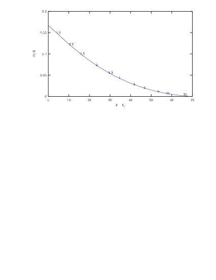
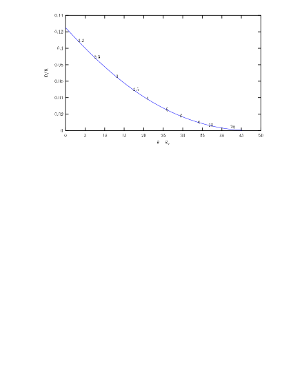
Figure 6: Plot of the maximum ratio $D/R$ as a function of the difference $\theta-\theta_{\star}$ where $\theta$ is the deflection angle and $\theta_{\star}$ is the maximum bending angle a jet can have in order not to produce a terminal shock. The plot refers to the points for which a shock at the beginning of the curvature (which was assumed to be a circle) has developed. Jets with parameters which lie below the curve in any case do not develop any internal shocks at all for this particular circular trajectory. The plot at the top was calculated using the results in which the gas is non–relativistic and its polytropic index is $5/3$. The plot at the bottom was made by considering the gas to be ultrarelativistic and relativistic effects in the bulk motion of the flow were taken into account. For this second plot, the polytropic index was assumed to be $4/3$. The numbers in each plot correspond to the values of the Mach number in the flow.

7 Discussion

The relativistic Mach angle is smaller for a given value of the velocity of the flow than its non–relativistic counterpart as was proved in section 3. This fact is extremely important when analysing the possibility of the intersection of different characteristics in a bent jet. This intersection is what gives rise to the creation of shock waves. For a relativistic flow, the characteristics, which make an angle equal to the Mach angle to the streamlines, are always beamed in the direction of the flow. Thus, when a jet starts to bend, the possibilities of intersection between some characteristic line in the curved jet and the ones before it curves, become more probable than for their non–relativistic counterpart.

This difference results in a severe overestimation of the maximum bending angle $\theta_{\text{max}}$ when a non–relativistic treatment is made to the problem. For example, Icke (1991) used the non–relativistic analysis in the discussion of the generation of internal shocks due to bending of jets. Using the non–relativistic equations described above, but with a polytropic index $\kappa=4/3$, the value for the maximum deflection angle is $\theta_{\text{max}}\!=\!$134.16\text{\,}\mathrm{\SIUnitSymbolDegree}$$. This is much greater than the value of $\theta_{\text{max}}\!=\!$74.21\text{\,}\mathrm{\SIUnitSymbolDegree}$$ obtained with a full relativistic treatment.

The analysis made by Icke (1991) is important for jets in which the microscopic motion of the flow inside the jet is relativistic, but the bulk motion of the flow is non–relativistic.

Radio trail sources (Begelman et al., 1984) show considerable bending of their jets with deflection angles of about $90\text{\,}\mathrm{\SIUnitSymbolDegree}$ in many cases. Since the bending is produced by the proper motion of the host galaxy with respect to the intergalactic medium, the deflection angle cannot be greater than $90\text{\,}\mathrm{\SIUnitSymbolDegree}$. The results presented in eq.(57) show that jets which have a relativistic equation of state and a bulk relativistic motion of the gas within its jet, cannot be deflected more than $\sim\!$50\text{\,}\mathrm{\SIUnitSymbolDegree}$$. Since the deflections of radio trail sources are greater than this value, this result would imply that most radio trail sources should generate shocks at the end of their curvature. However, observations (see for example Eilek et al., 1984; O’Dea, 1985; de Young, 1991, and references within) show that the velocity of the material of the jets $\lesssim 0.2\text{--}0.3\mathrm{\text{ $c_{0}$ }}$. Therefore, the bulk motion of the flow is non–relativistic, despite the fact that the gas inside the jet has a relativistic equation of state. As we saw before, this implies that the value of the maximum angle is $\theta_{\text{max}}=$134.16\text{\,}\mathrm{\SIUnitSymbolDegree}$$.

In other words, these type of jets develop a terminal shock if their jets bend more than $\sim\!$135\text{\,}\mathrm{\SIUnitSymbolDegree}$$. This seems to be the reason why radio trail sources are able to bend so much without resulting in an internal shock wave that could potentially cause disruption of its structure.

In a previous paper (Mendoza & Longair, 2001), we discussed the possibility of a bent jet in the radio galaxy 3C 34 using the observations of Best et al. (1997). According to these observations, the radio source lies more or less in the plane of the sky, and so, if the western radio jet is curved, this must be of the order of $10\text{\,}\mathrm{\SIUnitSymbolDegree}$. The value $\theta\sim$10\text{\,}\mathrm{\SIUnitSymbolDegree}$$ is well below the upper limit of $\sim$50\text{\,}\mathrm{\SIUnitSymbolDegree}$$ calculated in eq.(57), so that no terminal shock would be produced by the deflection of the jet. From the lower plot of Fig. 6 and because the angle $\theta_{\star}\!\ll\!1$ for a high relativistic flow, it follows that if the trajectory of the jet in 3C 34 is circular, then in order not to produce an internal shock at the onset of the curvature, the ratio $D/R$ has to be less than $\sim\!0.08$.

In the analysis made above, we have calculated how shocks can be generated inside a bent jet. These shocks are special in the sense that they do not reach the surface boundary of the jet. Instead they are generated away from the walls of the jet. For jets with an ultrarelativistic equation of state that possess a relativistic bulk motion, a shock is internally generated if they bend more than $\sim$50\text{\,}\mathrm{\SIUnitSymbolDegree}$$. If their bulk motion is non–relativistic, the shock is generated when the bending angle is more than $\sim$135\text{\,}\mathrm{\SIUnitSymbolDegree}$$. Jets with a polytropic index of $5/3$ that move non–relativistically generate a shock if the bending angle exceeds the value $\sim$50\text{\,}\mathrm{\SIUnitSymbolDegree}$$. These angles are only upper limits and the precise conditions under which a shock is produced have to be calculated individually. However using the diagrams presented in Fig. 6 and that presented by (Icke, 1991) it is possible to see if a shock is produced at the onset of the curvature.

All radio sources in which bendings of radio jets have been observed appear to satisfy the upper limits discussed above. So, it seems that jets are perhaps unstable if an internal shock is generated in a curvature. However, various observations and theoretical work in galactic and extragalactic sources (see for example Canto et al., 1989; Falle & Raga, 1993, 1995; Komissarov & Falle, 1998, and references within) show that internal shocks within a jet are a good mechanism that, under certain circumstances, can collimate the jets.

The question of whether an internal shock will lead to disruption of the jet is unknown and still a matter of debate. We aim to give to the problem an answer in a future paper.

8 Acknowledgements

SM would like to thank Paul Alexander for providing ideas to the problem discussed in this paper while giving a seminar at the Cavendish Laboratory in Cambridge. He also thanks support granted by the Cavendish Laboratory and the Dirección General de Asuntos del Personal Académico at the Universidad Nacional Autónoma de México.

References

- Begelman et al. (1984) Begelman M., Blandford R., Rees M., 1984, Rev. Mod. Phys., 56, 255
- Best et al. (1997) Best P. N., Longair M. S., Rottgering H. J. A., 1997, MNRAS, 286, 785
- Canto et al. (1989) Canto J., Raga A. C., Binette L., 1989, Revista Mexicana de Astronomia y Astrofisica, 17, 65
- Chiu (1973) Chiu H. H., 1973, Physics of Fluids, 16, 825
- Courant & Friedrichs (1976) Courant R., Friedrichs K., 1976, Supersonic Flow and Shock Waves. Applied mathematical sciences; vol.21, Interscience Publishers
- de Young (1991) de Young D. S., 1991, ApJ, 371, 69
- Eilek et al. (1984) Eilek J. A., Burns J. O., O’Dea C. P., Owen F. N., 1984, ApJ, 278, 37
- Falle & Raga (1993) Falle S. A. E. G., Raga A. C., 1993, MNRAS, 261, 573
- Falle & Raga (1995) Falle S. A. E. G., Raga A. C., 1995, MNRAS, 272, 785
- Icke (1991) Icke V., 1991, in Huges P. A., ed., Beams and Jets in Astrophysics. From nucleus to hotspot. Cambridge University Press, pp 232–277
- Kolosnitsyn & Stanyukovich (1984) Kolosnitsyn N. I., Stanyukovich K. P., 1984, PMM Journal of Applied Mathematics and Mechanics, 48, 96
- Komissarov & Falle (1998) Komissarov S. S., Falle S. A. E. G., 1998, MNRAS, 297, 1087
- Königl (1980) Königl A., 1980, Physics of Fluids, 23, 1083
- Landau & Lifshitz (1987) Landau L., Lifshitz E., 1987, Fluid Mechanics, 2nd edn. Vol. 6 of Course of Theoretical Physics, Pergamon
- Landau & Lifshitz (1994) Landau L., Lifshitz E., 1994, The Classical Theory of Fields, 4th edn. Vol. 2 of Course of Theoretical Physics, Pergamon
- Mendoza & Longair (2001) Mendoza S., Longair M. S., 2001, MNRAS, 324, 149
- O’Dea (1985) O’Dea C. P., 1985, ApJ, 295, 80
- Stanyuokovich (1960) Stanyuokovich K. P., 1960, Unsteady motion of continuous Media. Pergamon