Components of the Milky Way and GAIA

Abstract

The GAIA mission will produce an extraordinary database from which we should be able to deduce not only the Galaxy’s current structure, but also much of its history, and thus cast a powerful light on the way in which galaxies in general are made up of components, and of how these formed. The database can be fully exploited only by fitting to it a sophisticated model of the entire Galaxy. Steady-state models are of fundamental importance even though the Galaxy cannot be in a steady state. A very elaborate model of the Galaxy will be required to reproduce the great wealth of detail that GAIA will reveal. A systematic approach to model-building will be required if such a model is to be successfully constructed, however. The natural strategy is to proceed through a series of models of ever increasing elaborateness, and to be guided in the specification of the next model by mismatches between the data and the current model.

An approach to the dynamics of systems with steady gravitational potentials that we call the ‘torus programme’ promises to provide an appropriate framework within which to carry out the proposed modelling programme. The basic principles of this approach have been worked out in some detail and are summarized here. Some extensions will be required before the GAIA database can be successfully confronted. Other modelling techniques that might be employed are briefly examined.

1 Introduction

GAIA will provide at least 5 and often 6 phase-space coordinates for $10^{9}$ stars. The challenge is to make astrophysical sense of this vast dataset. Studies of external galaxies have convinced us that galaxies are best understood as being made up of a series of ‘components’: a bulge or ‘spheroid’ and perhaps a bar; a thin disk and perhaps a thick disk; a massive halo and perhaps a metal-poor halo. We must somehow use all those phase-space data to learn about the components of the Milky Way: how big are they? how old? what are their radial profiles and shapes? did they form slowly or suddenly? did some give rise to others?

Nearly all galaxies have a disk and a bulge, though the relative importance of these two components can vary greatly and largely determines the galaxy’s Hubble type. It is probable but not certain that nearly all galaxies have dark halos. A significant proportion of galaxies possess either a bar or a thick disk. Understanding how the different components of galaxies were formed, and why their relative prominence varies from galaxy to galaxy, are clearly central questions in the current drive to understand why there are galaxies at all, and the relationship of galaxies to the rest of the matter in the Universe. To answer these questions we need to have the most complete picture possible of what individual components are, how they the function dynamically, and how they fit together. The Milky Way, which is a prototype of the galaxies that are responsible for most of the luminosity in the Universe, is known to possess all the components listed above, and kinematic mapping of these with GAIA offers a unique opportunity to clarify some of the fundamental questions of contemporary astronomy.

Interpreting the GAIA database in terms of components is a thoroughly non-trivial task because components are coextensive at many locations, both in real space and in theoretical spaces in which a kinematic or chemical datum is used as a coordinate. So it will often be impossible to assign unambiguously an individual star to this or that component: at best we will be able to give probabilities for its belonging to one or another component. Moreover, in the assignment of these probabilities we encounter the chicken-and-egg problem: until we have assigned stars to components, we will have a very imperfect knowledge of each component’s chemical composition and dynamics and we will not be in a position to say how a star’s membership probability varies as a function of its chemical and kinematic data.

For these reasons a major intellectual and computational effort will be required to pass from the GAIA database to a knowledge of the structure and dynamics of the Galaxy’s components.

2 The steady-state approximation

All components are held together by the Galaxy’s gravitational potential $\Phi$, which is currently extremely ill-determined at points away from the Galactic plane. A successful attempt to model the various components will inevitably yield, almost as a spin-off, a good knowledge of $\Phi$ throughout the visible Galaxy. Taking the Laplacian of $\Phi$ and subtracting the mass densities of the visible components, we will finally determine unambiguously the distribution of Galactic dark matter.

The physical principle that will enable us to determine $\Phi$ is that the Galaxy is in an almost steady state. This assumption, which is only approximately valid, merits a moment’s consideration. We think the Galaxy should be in an approximately steady state because throughout the visible Galaxy the dynamical time is orders of magnitude shorter than the Hubble time, and we have no reason to suppose this is a particularly exciting moment in the Galaxy’s life, such as the climax of a major merger. However, various processes that are incompatible with a steady state should be detectable.

One factor is the bar: deviations from steadiness will be significant unless we refer everything to the bar’s rotating frame. The pattern speed of this frame is not exactly known, although Dehnen [1] gives a reasonably precise value. The bar is almost certainly losing angular momentum to other components, with the result that it is slowing down and the other components are heating up. Since bars such as the Galaxy’s are extremely common in disk galaxies, these processes are probably slow and lead to only small violations of the steady-state principle. The violations are likely to be detectable, however.

Spiral structure must be redistributing angular momentum within the disk, and heating it. This process should lead to small but detectable violations of the steady-state principle.

The Galaxy is accreting angular momentum that is not aligned with its current spin axis. This accretion is in the long run expected to lead to significant reorientation of the spin axis [2], and in the shorter term probably generates the Galactic warp [3], whose kinematic signature Hipparcos reliably detected for the first time [4].

Finally, the Galaxy is constantly tidally stripping small fry that come too close and the debris of such stripping will not be in a steady state [5, 6].

Notwithstanding these process that violate the stead-state approximation, the latter is a vital tool in the determination of $\Phi$. To see why, consider the consequence of modelling the GAIA database with a potential that is much less deep than the true potential. In this case, when the equations of motion of stars are integrated from the initial conditions that GAIA provides, the Galaxy will fly apart into intergalactic space. Similarly, if the adopted potential is too deep, integration of the equations of motion will result in the Galaxy contracting on a dynamical time, and if the potential’s flattening towards the plane is incorrect, the halo and thick disk will change shape in the first dynamical time. The true potential is the one that make the observed stellar distribution pretty much invariant under integration of the equations of motion.

The idea just described, of integrating the equations of motion forward from the initial conditions that GAIA will provide, illustrates the physical idea behind potential estimation, but it is not likely to be useful in practice. The main reason is that obscuration will prevent GAIA from observing the entire Galaxy. Moreover, stars less luminous than the horizontal branch will not be picked up throughout the Galaxy. If we take the correct potential and integrate the equations of motion from initial conditions yielded by such an incomplete survey, the star distribution will not be invariant: many of the low-luminosity stars that GAIA sees near the Sun will wander off and will not be replaced because the stars that should replace them were initially too far away to be seen by GAIA; stars will move into obscured zones, and gaps in the observed regions will open because they will not be replaced by stars moving out of obscured zones. Some more sophisticated procedure is going to be required to test whether the GAIA data are compatible with the steady-state approximation in a given potential.

3 The torus project

Similar problems arise in accentuated form when one tries to model ground-based data. Some years ago my group in Oxford started work on a way of modelling the Milky Way that promises to overcome these problems [7]. Our work was interrupted by the arrival of the first Hipparcos data and is only now resuming. It will be disappointing indeed if the project has not been completed by the time GAIA flies, so I will outline it.

We start from the premise that for any trial potential $\Phi$ we should have a strictly steady-state dynamical model of each component. We recognize that real components will not be in exactly steady states, but argue that the best method of identifying the effects of unsteadiness in the data is comparison with the best-fitting steady-state model. Moreover, we hope to be able to model unsteadiness by perturbing our steady-state model.

Jeans’ theorem tells us that a steady-state model of a component may be generated by taking the component’s distribution function (DF) $f_{\alpha}$ to be an arbitrary non-negative function of the potential’s isolating integrals. If the potential were ‘integrable’ it would possess just three functionally independent isolating integrals, and the DF would be a function of three variables. That is, each component would correspond to a particular distribution of stars in a three-dimensional space, and the observed distribution of stars in six-dimensional phase space could in principle be read off from the function of three variables, just as a living organism can be constructed from its DNA sequence.

Several practical difficulties have to be overcome before we can exploit this dramatic simplification. One is that isolating integrals are by no means unique: a function of two or more isolating integrals is itself an isolating integral. If we are to talk intelligently about the differences between the DFs of different components, or the DFs of the same component in different trial potentials, we must standardize our isolating integrals. This is readily done by using only action integrals (e.g., §3.5 of [8]). For an integrable potential these suffer only from a trivial degree of ambiguity, which is readily eliminated. For an axisymmetric potential our standard actions are the radial action $J_{R}$, the latitudinal action $J_{l}$ and the azimuthal angular momentum $J_{\phi}$. The space that has these actions for Cartesian coordinates we call ‘action space’.

In addition to being unambiguously defined for any integrable potential, actions have the desirable property of faithfully mapping phase space into action space, in the sense that the volume of phase space occupied by orbits with actions in the action-space volume ${\rm d}^{3}{\bf J}$ is $(2\pi)^{3}{\rm d}^{3}{\bf J}$. Consequently, the DF of a component may be considered to be the density of stars in action space [up to a factor $(2\pi)^{-3}$] as much as it is the density of stars in phase space.

Unfortunately, a generic potential will typically not admit three global isolating integrals, and even if it does, we will not have analytic expressions for the functions $J_{i}({\bf r},\dot{\bf r})$ that relate phase space to action space. Over a number of years my group has developed solutions to this problem [9, 10, 11, 12, 13]. In an integrable potential, the surfaces in phase space on which actions are constant are topologically 3-tori. On these surfaces the Hamiltonian is constant, and all surface integrals of the form $\int{\rm d}{\bf p}.{\rm d}{\bf q}$ vanish, so they are called ‘null-tori’. Stars move over these null-tori in a rather special way – each torus admits three variables, the ‘angle variables’ $\theta_{i}$, that are canonically conjugate to the actions that label the tori, and these angles increase uniformly in time: $\theta_{i}(t)=\theta_{i}(0)+\omega_{i}t$. Unless the frequencies $\omega_{i}$ are commensurable, it follows that in a steady-state model the phase-space density of stars is constant over a torus: this is the origin of Jeans’ result that the DF of a steady-state model does not depend on the $\theta_{i}$.

It turns out that if all phase space can be foliated by such null 3-tori, and the given Hamiltonian $H$ is constant on them, then $H$ is integrable, and its actions label the tori by giving the magnitudes of their three independent cross-sectional areas, $J_{i}=(2\pi)^{-1}\oint_{i}{\bf p}.{\rm d}{\bf q}$. We have developed a technique for foliating phase space with null tori on which a given $H$ is nearly constant. These tori can be used to define a integrable Hamiltonian $\hat{H}$ that differs from $H$ by only a small amount.

3.1 Resonances & perturbation theory

A real galactic potential is exceedingly unlikely to be integrable in the sense that it admits a global set of angle-action variables. Consequently, the integrable Hamiltonian $\hat{H}$ will surely differ from the true Hamiltonian $H$ at some level. Since $\delta H=H-\hat{H}$ is small compared to $H$, stars integrated in $H$ and $\hat{H}$ from the same initial condition will stay close to one another for a few orbital times. In fact, the motion in the true Hamiltonian $H$ can be considered to be the result of perturbing the integrable Hamiltonian $\hat{H}$ by $\delta H=H-\hat{H}$. The astronomical significance of this perturbation will depend on the age of the system measured in dynamical times and whether orbits of interest lie near a resonance of $\hat{H}$: if the initial conditions lie on a resonant torus, even the small perturbation $\delta H$ can cause the orbit in $H$ to deviate significantly from that in $\hat{H}$ if you wait long enough. Consequently, the phenomena occurring in $H$ can differ significantly from those occurring in $\hat{H}$, and it may be necessary to obtain a better approximation to the true dynamics than $\hat{H}$ provides.

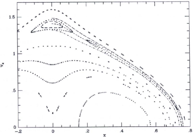
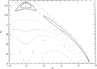
Figure 1: A surface of section for motion in a barred potential. Dots show consequents of numerically integrated orbits. In a band towards the outside of the figure, these delineate a chain of islands. At left three dashed curves through these islands show cross sections of tori of the underlying integrable Hamiltonian $\hat{H}$. At right the full curves that accurately delineate the islands are obtained by treating $\delta H$ as a perturbation on $\hat{H}$. (From [14])

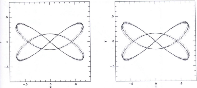
Figure 2: One of the 2:3 resonant box orbits that generate the chain of islands in Figure 1. The orbit shown at left was generated by direct integration, while that at right was generated by applying perturbation theory to the integrable Hamiltonian $\hat{H}$. The full curve is the underlying closed orbit. (From [14])

The torus programme offers two ways of improving on the model provided by $\hat{H}$. The left panel of Figure 1 illustrates one method by showing part of a surface of section. The figure’s dots are the consequents of eight orbits in a barred gravitational potential. These orbits all admit an isolating integral in addition to $H$ because their consequents lie on smooth curves. Six of these curves have the characteristic shapes of the invariant curves of box and loop orbits (e.g., Fig. 3-8 in [8]), which are associated with a global system of action-angle coordinates (§3-5 of [8]). Just inside the outer-most invariant curve, the invariant curves have a different structure, forming part of what would be a chain of six islands if the whole surface of section were plotted. The torus machinery has been used to draw three dashed curves through the region occupied by the islands: one curve goes through the middle of the islands, while flanking curves pass either side of them. These curves are invariant curves of $\hat{H}$, which admits global action-angle coordinates and therefore supports only boxes and loops.

The right panel of Figure 1 shows the same surface of section, but now with the islands delineated by full curves. These curves are generated by treating $\delta H$ as a perturbation of $\hat{H}$. Since $\delta H/H$ is small, the agreement between the numerical consequents and the invariant curves from first-order perturbation theory is excellent. Figure 2 shows that in real space one cannot distinguish between the orbits obtained by direct integration and perturbation theory.

Figure 3 shows an alternative approach to resonant orbits, which is appropriate when the resonance is powerful, and therefore $\delta H/H$ is not small. The left panel again shows invariant curves of $\hat{H}$ ploughing through the resonant region, which is now associated with non-negligible stochasticity near the seperatrices. The right panel shows excellent agreement between consequents for a series of resonant orbits and invariant curves obtained by generating a new integral hamiltonian $\hat{H}^{\prime}$ for the resonant region. This Hamiltonian is obtained by assuming that tori have the general structure required for libration about the closed resonant orbit, and then deforming them so as to make $H$ as nearly constant over them as possible.

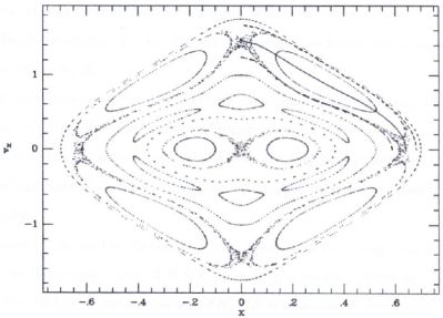
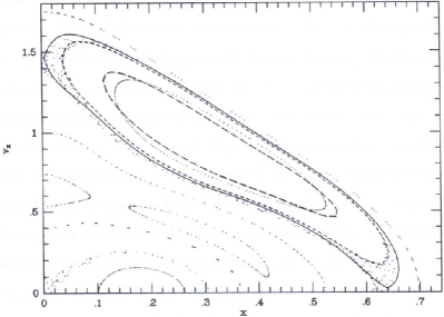
Figure 3: A surface of section in a barred potential in which most orbits are resonant boxes (‘boxlets’). The curves in the left panel shows the tori generated if all orbits are assumed to be non-resonant boxes. The curves in the right panel shows the tori obtained when orbits are assumed to be resonant. (From [14])

These examples show that the torus programme can, in principle, provide an extremely accurate description of regular orbits, no matter what their structure. The ability of the programme to give a good account of stochastic orbits has not been so completely explored. I anticipate, however, that it will prove powerful in this area also, since, as Figure 3 illustrates, it can provide a system of action-angle variables in which the stochastic region is bounded by particular tori. Let us call the values taken by ${\bf J}$ on these tori the ‘critical actions’. It is likely that over time the DF will tend to a function of energy only in the region of action space that is bounded by the critical actions.

3.2 Galaxy modelling with tori

Our procedure for interpreting a data set such as GAIA will produce is as follows. We start with a trial potential $\Phi({\bf r})$. We foliate phase space with 3-tori on which $H=\frac{1}{2}{\dot{r}}^{2}+\Phi({\bf r})$ is nearly constant. This foliation establishes a system of action-angle coordinates for an integrable Hamiltonian $\hat{H}$ that differs from $H$ only slightly. Routines are then available to pass between these action-angle coordinates and the ordinary Cartesian coordinates for phase space, $({\bf r},\dot{\bf r})$.

Next, for each component $\alpha$ of the Galaxy we choose a simple analytic DF $f_{\alpha}({\bf J})$. Because the actions are unique and physically well-motivated variables, it is easy to understand the relationship between the form of $f_{\alpha}$ and the observables of the component, such as its flattening, characteristic spin and the typical eccentricity of its stellar orbits [15]. Finally, for each component we choose an Initial Mass Function and a star-formation history, which together enable us to predict the distribution in colour and absolute magnitude of the component’s stars.

We now have a steady-state dynamical model of each component in the given $\Phi$. This model predicts the probability of observing a star of a given component at any phase space location. By convolving this probability distribution with the assumed colour and absolute-magnitude distributions of the component, and summing over components, we convert these probabilities into the probability of finding a star of given colour and $M_{V}$ at any point in phase space. Finally, these probabilities are convolved with the selection functions in colour and phase space of any given survey. This final probability distribution is then evaluated at the location of each catalogued star and the resulting numbers are multiplied together to give the likelihood of the catalogue given the current Galaxy model. We propose to maximize this likelihood by adjusting a suitably parameterized form of the Galactic potential $\Phi({\bf r})$ as well as the functions that characterize each component: the function of three variables $f_{\alpha}({\bf J})$, the IMF and the star-formation history. This maximization is likely to be a computationally challenging task, but not one that is out of proportion to the other computational challenges that GAIA inherently poses. Notice that the final model will encode not only the current state of the Galaxy, but much information about its past. Some more detail and sample calculations can be found in [7].

4 Other modelling techniques

It is not self-evident that the approach just described to modelling the GAIA database will be the most important one in practice, but it does contain a number of elements that any viable technique is likely to include.

First, I believe it is essential to produce a steady-state model of the Galaxy. Such a model is an unrealized ideal, but a key step both in the determination of the Galactic potential, and in deducing what features in the data are symptomatic of unsteady dynamics.

Second, one has somehow to extrapolate the stellar distribution from the parts of the Galaxy that are observed, to those that are not. The strategy suggested above for doing this is three-fold. First Jeans’ theorem is used to argue that if I observe the stellar density at one point in phase space, I know the density at all other points in phase space at which the isolating integrals take the same values. For hotter components, such as the halo and the thick disk, this argument allows one to determine even from observations confined to the solar neighbourhood, the value of the DF through a surprisingly large part of phase space [16]. For more luminous stars, GAIA’s coverage will be so extensive that this principle will be very powerful indeed. Second, the theory of stellar evolution and nucleosynthesis is used to connect the phase-space densities of faint stars to those of their more luminous brethren. Finally, the uniqueness of the action integrals is used to reduce the DF of each component to an analytic function of the actions that depends on a small number of parameters. This reduction not only simplifies the computational task of optimizing the DFs, but also facilitates astrophysical interpretation of the results.

4.1 Schwarzschild’s modelling technique

A widely used technique for modelling external galaxies is that of Schwarzschild [17, 18] and it is interesting to examine the possibility of using this to model the GAIA database. In Schwarzschild’s method one again starts with a trial potential $\Phi$, but one integrates a large number of orbits in it instead of constructing tori for it. Then, instead of choosing a DF $f_{\alpha}$ for each component, one chooses a set of weights $w^{(i)}_{\alpha}$ for each orbit $i$. The merit of the method is that orbit integration is computationally simple, and uses routines that are completely independent of the nature of the orbits: whether they are tube or box orbits, regular or stochastic. Torus construction, by contrast, has to be tuned to the dominant orbit families. Moreover, Schwarzschild’s method deals properly with families of resonant orbits whereas torus construction sweeps these under the rug for possible subsequent examination by perturbation theory.

Schwarzschild’s method has several weaknesses, however. One is that it is cumbersome numerically because phase-space points have to be stored at many points along each orbit, with the result that an ‘orbit library’ of 10,000 orbits will occupy of order $1\,$Gb on disk. Moreover, the resolution in space and velocity of the final model is determined by the number of orbits and the temporal frequency at which each is sampled. In the torus method, by contrast, each torus is represented by a relatively small number of expansion coefficients from which phase-space points can be evaluated dynamically as the model is compared to the data. There is no limit to how densely a given torus is sampled, and once a reasonable torus library is to hand, additional tori can be quickly constructed without reference to the Hamiltonian by interpolation on the expansion coefficients for nearby tori in the library. Finally, in its classical form Schwarzschild’s method gives no insight into which orbits are ‘close’ to each other in phase space. This has two consequences. One is that there is no way of requiring the weights of neighbouring orbits to be nearly equal, as seems physically reasonable. The other is that one cannot determine the density of a component at a given point in phase space, which makes it impossible to compare the phase-space structure of models built with different orbit libraries, even if the potentials are identical. In fact, communication of a model requires transmission of both the $\sim 1\,$Gb of the orbit library and a complete set of orbit weights ($\sim 100\,$Kb per component). By contrast, a model constructed by the torus method can be communicated by tabulating the four or five parameters in the DF of each component.

Häfner et al [19] show how Schwarzschild’s method may be upgraded to the point at which it returns the DF at the location of each orbit. Moreover following Zhao [20], one can assign ‘effective integrals’ to each orbit which enable one to say, in an approximate way, which orbits are close to one another, and thus impose continuity of the DF. Moreover, one could insist that the weights were those implied by an analytic function of the effective integrals that depends on a small number of parameters, in the same way that the torus method assumes the DF to be a parameterized function of the actions. Used in this mode, Schwarzschild’s method could be equal to the task of modelling the GAIA data set.

4.2 N-body models

Fux [21] has made a significant contribution to our understanding of the dynamics of the inner Galaxy simply by observing a suitable $N$-body model. Could this approach make a significant contribution to our understanding of the GAIA dataset? If we were to set up an $N$-body model simply by using the coordinates returned by GAIA as initial conditions, we would run up against the problems with observational selection that were described above. A better way of choosing initial conditions would be to start by fitting to the GAIA data to DFs of the form $f_{\alpha}({\bf r},\dot{\bf r})=\rho_{\alpha}({\bf r})p_{\alpha}(\dot{\bf r})$, where $\rho_{\alpha}$ is an analytic fit to the density distribution of component $\alpha$ and $p_{\alpha}$ is an analytic probability density that approximately describes the distribution of velocities within this component. For judiciously chosen $\rho_{\alpha}$ and $p_{\alpha}$ the initial conditions might soon settle to a steady-state that resembled the Galaxy. Setting up an $N$-body model in this way would be by no means trivial, however, because choosing the functions $p_{\alpha}(\dot{\bf r})$ is likely to be a delicate business. The technique devised by Syer & Tremaine [22], in which the masses of particles are dynamically adjusted, may be able to make up for short-comings in the choice of the $p_{\alpha}$.

All of these particle-based schemes – Schwarzschild’s technique, and N-body modelling with or without the refinements of Syer & Tremaine – will suffer from the drawback that, for feasible numbers of masses in the model, errors in the model’s observables, such as velocity distributions near the Sun, will far exceed those in the data. Consequently, none of these schemes is likely to do justice to the precision of the GAIA data.

5 Conclusion

GAIA poses an enormous challenge to the theorist because it is essential that its vast data set be modelled as a whole and in a single sweep. The modelling must include not only the dynamics of the contemporary Galaxy, but many aspects of its history as well, most particularly the star-formation history of its various components.

In view of the scale of this enterprise, it is fortunate that the data will not arrive for more than a decade. In that period Moore’s law for the growth of computer power will ensure that the necessary computational resources will be available. If we start now, there is a reasonable chance that appropriate computational schemes will also be on hand for modelling the Galaxy in the requisite depth and breadth. Developing these schemes will be astronomically rewarding in the short term also, since there is an abundance of ground-based data to model that poses the same conceptual problems in heightened form.

The richness of the GAIA database will ultimately allow us to study the Galaxy in exquisite detail, and to learn about the various chance events that have cumulatively shaped it. Extracting this detail from the database will require subtlety, however, and it is likely the that best strategy for mining the database will be one in which models of systematically increasing sophistication are successively fitted to the data. The first models would assume that the Galaxy has a globally integrable potential and is in a strictly steady state. Discrepancies between the data and the best-fitting model of this type might indicate that certain resonances are not to be ignored. At the next level a model that included these resonances but was still in a strictly steady-state would be fitted to the data. Discrepancies between model and data might now point to non-steady phenomena such as spiral structure. Perturbation theory would then be used to model these effects, and discrepancies again sought. Proceeding in this manner one can imagining constructing a very detailed model that reflected many of the chance events that have fashioned the Galaxy, as well as ongoing evolution driven by the bar, spiral structure and the Sagittarius dwarf galaxy.

The torus programme has a number of features that suit it very well to this programme of work. Most importantly, it allows one to start with an extremely simple model that can be described by only a handful of parameters, and to upgrade this model through a systematic sequence of well defined stages. At each stage, the model fitted to the data at the preceding stage provides a clear basis from which to advance to a more elaborate model. Another important advantage of the torus programme is the facility to beat discreteness noise down to any predefined value in a straightforward way.

A number of published papers demonstrate the basic principles of the torus programme for the case of two-dimensional potentials, which effectively includes all three-dimensional axisymmetric potentials. The generalization of these principles to general, nearly integrable, three-dimensional potentials is straightforward though computationally costly. Important tasks that must be accomplished before the torus programme can be applied to the GAIA database include exploring its application to chaotic orbits and, through perturbation theory, to non-steady systems.

References

- [1] Dehnen, W., ApJ, 524, L35 (1999)
- [2] Binney, J. & May, A., MNRAS, 218, 743 (1986)
- [3] Jiang, I.-G. & Binney, J., MNRAS, 303, L7 (1999)
- [4] Dehnen, W., AJ, 115, 2384 (1998)
- [5] Helmi, A., White, S.D.M., de Zeeuw, P.T. & Zhao, H.-S. Nature, 402, 53 (1999)
- [6] Ibata, R., Irwin, M., Lewis, G.F. & Stolte, A., ApJ, 547, L133 (2000)
- [7] Dehnen, W. & Binney, J., in ‘Formation of the Galactic Halo…Inside and Out’, ASP Conference Series, Vol. 92, Heather Morrison and Ata Sarajedini, eds., p. 393 (1996)
- [8] Binney, J. & Tremaine, S., ‘Galactic Dynamics’, Princeton University Press, (1987)
- [9] McGill, C. & Binney, J., MNRAS, 244, 634 (1990)
- [10] Binney, J. & Kumar, S. MNRAS, 261, 584 (1993)
- [11] Kaasalainen, M. & Binney, J., MNRAS, 268, 1033 (1994)
- [12] Kaasalainen, M. & Binney, J., Phys. Rev. L., 73, 2377 (1994)
- [13] Kaasalainen, M., MNRAS, 275, 162 (1995)
- [14] Kaasalainen, M., Oxford University DPhil thesis (1994)
- [15] Binney, J. in ‘Galactic and solar system optical astrometry’, ed. L. Morrison, Cambridge University Press, p. 141 (1994)
- [16] May, A. & Binney, J., MNRAS, 221, 857 (1986)
- [17] Schwarzschild, M., ApJ, 232, 236 (1979)
- [18] Schwarzschild, M., ApJ, 263, 599 (1982)
- [19] Häfner, R., Evans, N.W., Dehnen, W. & Binney, J., MNRAS, 314, 433 (2000)
- [20] Zhao, H.-S., MNRAS, 283, 149 (1996)
- [21] Fux, R., A&A, 345, 787 (1999)
- [22] Syer, D. & Tremaine, S., MNRAS, 282, 223 (1996)