Planetary nebulae as mass tracers of their parent galaxies: biases in the estimate of the kinematical quantities

Abstract

Multi-object and multi-fiber spectrographs on 4 and 8 meter telescopes make it possible to use extragalactic planetary nebulae (PNe) in the outer halos of early-type galaxies as kinematical tracers, where classical techniques based on integrated stellar light fail. Until now, published PNe radial velocity samples are small, with only a few tens of radial velocity measurements (except for a few cases like NGC 5128 or M31), causing uncertainties in the mass and angular momentum estimates based on these data. To quantify these uncertainties, we have made equilibrium models for spherical galaxies, with and without dark matter, and via Montecarlo simulations we produce radial velocity samples with different sizes. We then apply, to these discrete radial velocity fields, the same standard kinematical analysis as it is commonly done with small samples of observed PNe radial velocities. By comparison of the inferred quantities with those computed from the analytical model, we test for systematic biases and establish a robust procedure to infer the angular momentum distribution and radial velocity dispersion profiles from such samples.

1 Introduction

The dynamics of the outer regions of early-type galaxies have been studied by means of test particles like globular clusters (GCs) and planetary nebulae (PNe). GCs have been successfully used to probe the gravitational potential in giant ellipticals (M87: Mould et al. [1990]; Cohen [2000]; NGC5128: Sharples [1988]; Harris et al. [1988]; NGC1399: Grillmair et al. [1994]; Minniti et al. [1998]; Kissler-Patig et al. [1998]), but their number density and angular momentum distributions often turn out to be different from those of the stellar population in the outer galaxy halos.

PNe are a population of dying stars, whose outer envelope re-emits more than 15% of the energy emitted in the UV by the internal star in the [OIII] green line at 5007 Å  (Dopita et al. [1992]) and therefore they can be readily detected in distant galaxies. The observational evidences indicate that the number density of PNe, unlike GCs, is proportional to the underlying stellar light (Ciardullo et al. [1989]; Ciardullo et al. [1991]; McMillan et al. [1993]; Ford et al. [1996]) and they share the angular momentum distribution of the stars (Arnaboldi et al. [1994]; Hui et al. [1995]; Arnaboldi et al. [1996], [1998]). First attempts to use PNe as kinematical tracers in nearby galactic systems date back to 1986 (Nolthenius & Ford [1987]) and studies of early-type systems within a distance of 10 Mpc rapidly followed (Ciardullo et al. [1993]; Tremblay et al. [1995]; Hui et al. [1995]). Since 1993 new observing techniques (eg Arnaboldi et al. [1994]) allowed measurements of radial velocities of PNe in the outer regions of giant early-type galaxies situated at distances larger than 10 Mpc. These studies, mostly based on samples of only a few tens of PNe, show that the outer PNe typically have faster systemic rotation than GCs (Grillmair et al. [1994]; Arnaboldi et al. [1994]; Hui et al. [1995]; Arnaboldi et al. [1998]).

So far these small samples were analysed by adopting simple three-parameter functions for the underlying projected rotation field, but no detailed studies have yet been reported to test for biases in the estimated rotation and velocity dispersion introduced by these adopted (parametric) functions. Non-parametric analyses can in principle avoid this problem. In practice, however, for the small data samples of interest here, the associated inherent smoothing effectively drives the non-parametric analysis towards one of the commonly used simple parametric forms (like solid body rotation: see for example Arnaboldi et al. [1998]).

In the large telescope era, much larger samples of PNe velocities will become available for galaxies out to distances of about 20 Mpc. The question of biases induced by adopting simple parametric forms for the rotation field remains relevant, because studies of galaxies at larger distances will still be limited to small sample of radial velocities. It will be important to know how to compare the results for nearby giant ellipticals, based on large samples of PNe velocities, with those for more distant objects, based on smaller samples.

In this paper we build simple equilibrium models with and without dark matter (DM) for spherical early-type galaxies (Sect. 2). Via Montecarlo simulations, we extract samples of tracers of various sizes (Sect. 3). We then adopt simple forms for the mean rotation field and derive the parameters for the projected 2-D rotation velocity field from these samples (Sect. 4 and 5). We also derive estimates of the precision and biases for the mean rotation and velocity dispersion (Sect. 6 and 7). The main goal of this work is to determine the minimum sample needed to derive reliable estimates of the kinematics of the host system via these parametric fits, and to define a robust approach to derive observables from small radial velocity samples. Discussion and conclusions are drawn in Sect. 8.

2 Analytical spherical systems in equilibrium

In our modeling we wish to represent the characteristics of the observed PNe distribution in early-type galaxies. In these systems, the observed PNe number density follows the stellar light distribution (Ciardullo et al. [1989]; Ciardullo et al. [1991]; McMillan et al. [1993]; Ford et al. [1996]), except in the bright inner regions where the PNe counts become incomplete. As the surface brightness of the stellar continuum background increases towards small radii, the 5007 Å [OIII] emission from the PNe is more difficult to detect and the apparent ratio of PNe to luminosity decreases. In Appendix, we compute the value of the limiting radius $R_{\mathrm{lim}}$ for which at large radii the PNe sample is complete. For the surface brightness profile of a typical E galaxy in Virgo Cluster, we find that $R_{\mathrm{lim}}=0.7\times R_{\mathrm{e}}$, where $R_{\mathrm{e}}$ is the effective radius.

2.1 Systems without dark matter

Assuming constant mass to light ratio (M/L), the analytic Hernquist ([1990]) model is a good approximation to a system whose surface brightness distribution follows the de Vaucouleurs law ([1948]). The luminous mass density is given by:

$$\rho(r)=C_{\mathrm{l}}\frac{M_{\mathrm{l}}a}{2\pi}\frac{1}{r(r+a)^{3}}\mbox{,}$$ (1)

where $M_{\mathrm{l}}$ is the total luminous mass, $a$ is a distance scale ($R_{\mathrm{e}}=1.8153~{}a$) and $C_{\mathrm{l}}$ is a normalization constant. We consider systems truncated at $R_{\mathrm{max}}=18a$ (i.e. $\sim 10R_{\mathrm{e}}$). For $a=1$ and $M_{\mathrm{l}}=1$, the normalization constant $C_{\mathrm{l}}=1.114$. Writing $r$ for $r/a$, we define a dimensionless density distribution

$$\tilde{\rho}(r)=\left\{\begin{array}[]{lll}\frac{C_{\mathrm{l}}}{2\pi}\frac{1}{r(r+1)^{3}}&&r\leq 18\\ 0&&r>18\end{array}\right..$$ (2)

The cumulative mass distribution is then

$$M_{\mathrm{l}}(r)=4\pi\int_{0}^{r}x^{2}\rho(x)dx.$$ (3)

The test particles are extracted from this distribution, taking into account the incompleteness effects at radii $\leq R_{\mathrm{lim}}$. We then consider the kinematics of PNe within $10a=5.5R_{\mathrm{e}}$, corresponding to the typical radial coverage of the observed PNe samples in real galaxies.

2.1.1 Systems with dark matter

In constructing our equilibrium models, we also consider systems with an additional mass contribution to the stellar mass density coming from a dark halo. Furthermore we model the dark halo with a Hernquist mass distribution, with scale length large enough so that it roughly mimics a $\rho\sim r^{-2}$ halo in the region of interest ($r<10$). We write the dark matter density as

$$\rho_{\mathrm{d}}(r)=\frac{M_{\mathrm{d}}d}{2\pi}\frac{1}{r(r+d)^{3}}$$ (4)

and adopt $d=10a$ and $M_{\mathrm{d}}=7.7M_{\mathrm{l}}$ (in agreement with the mass distribution of NGC5128, Hui et al. [1995]). The cumulative mass distribution is defined as in Eq. (3), and the potential is derived from the total mass

$$M_{\mathrm{t}}(r)=M_{\mathrm{l}}(r)+M_{\mathrm{d}}(r).$$ (5)

The $M_{\mathrm{l}}(r)$, $M_{\mathrm{d}}(r)$ and $M_{\mathrm{t}}(r)$ distribution are shown in Fig. 1.

Figure 1: Mass distributions for the Hernquist model: luminous mass matter (dash-dotted line), dark halo mass (dashed line) and the total mass (solid line).

2.2 Intrinsic and projected kinematics

We consider non-rotating and rotating equilibrium spherical systems, with the velocity dispersion components given by the Jeans equations.
For non-rotating systems with no dark matter, we assume that mass follows light and adopt an isotropic velocity dispersion to solve the radial Jeans equation

$$\frac{d(\rho\sigma^{2})}{dr}=-G\frac{M_{\mathrm{l}}(r)\rho(r)}{r^{2}}.$$ (6)

The solution in this simple case is

$$\begin{array}[]{rl}\sigma^{2}(r)=&7.110^{-7}r(1.+r)^{3}\{-0.13-\\ &[130321(1+r)^{-4}(25+52r+42r^{2}+12r^{3}\\ &+12(1+r)^{4}\log(r)-12(1+r)^{4}\log(1+r))]\}\end{array}$$ (7)

where $\sigma(r)$ is given in units of $v_{\mathrm{g}}=\sqrt{GM_{\mathrm{l}}/a}$⁽⁾.

We should also investigate rotating systems because early-type galaxies appear to show fast rotation in their outer parts (Hui et al. [1995]; Arnaboldi et al. [1996], [1998]). What is the most appropriate form for the rotation law ? The only system for which a mean stellar rotation law has been derived reliably out to large radii is Centaurus A. Here, Hui et al. ([1995]) adopt the functional form

$$v_{\mathrm{rot}}(R)=\frac{V_{\mathrm{max}}R}{\sqrt{R^{2}+R_{\mathrm{v}}^{2}}},$$ (8)

where $R$ is the distance from the galactic center and $R_{\mathrm{v}}$ a scale distance, which reproduces the rotation of NGC5128 in its equatorial plane. We assume that our model systems have the same underlying rotation law, and adopt a cylindrical rotational structure with the same functional form, where $R$ is now the radial coordinate in a cylindrical ($R$, $\varphi$, $z$) system.

In a conventional cylindrical coordinate system, ($R$, $\varphi$, $z$), the Jeans equations become

$$\frac{\partial\rho\overline{v_{R}^{2}}}{\partial R}+\rho\left(\frac{\overline{v_{R}^{2}}-\overline{v_{\varphi}^{2}}}{R}+\frac{\partial\Phi}{\partial R}\right)=0\mbox{ and}$$ (9)

$$\frac{\partial\rho\overline{v_{z}^{2}}}{\partial z}+\rho\frac{\partial\Phi}{\partial z}=0,$$ (10)

where $\rho$ and $\Phi$ are functions of ($R$, $z$).

If we substitute into equation (9) a given cylindrical rotation law, and assume an isotropic velocity dispersion, then this system is over-determined. If we now relax the condition of isotropy and assume that the principal axes of the velocity ellipsoid lie parallel to the ($R$, $z$) axes and $\sigma_{R}^{2}=\sigma_{\varphi}^{2}\neq\sigma_{z}^{2}$, the system of equations can be written as

$$\begin{array}[]{ll}\frac{\partial\rho(R,z)\sigma_{R}^{2}(R,z)}{\partial R}-\frac{\rho(R,z)}{R}v_{\mathrm{rot}}^{2}(R)=&\\ &\\ ~{}~{}~{}~{}~{}~{}~{}~{}~{}~{}~{}~{}~{}~{}~{}~{}~{}~{}~{}~{}~{}=-\rho(R,z)\frac{\partial\Phi(R,z)}{\partial R}&\mbox{ and}\end{array}$$ (11)

$${\footnotesize\frac{\partial\rho(R,z)\sigma_{z}^{2}(R,z)}{\partial z}=-\rho(R,z)\frac{\partial\Phi(R,z)}{\partial z}}.$$ (12)

These two equations can be solved independently by simple inversion as in Binney & Tremaine ([1987]). We believe this to be a reasonable approach for our purpose. It describes an equilibrium system with a spherical potential and a given cylindrical rotation law of known functional form.

Physically plausible solutions require that the components of the velocity ellipsoid are all positive in the volume occupied by the system. As we will see later, only certain values of $V_{\mathrm{max}}$ in Eq. (8) allow physical solutions in the whole volume occupied by the system. In Fig. 2 we show the intrinsic kinematics for $V_{\mathrm{max}}=0.23v_{\mathrm{g}}$ and $R_{\mathrm{v}}=2a$.

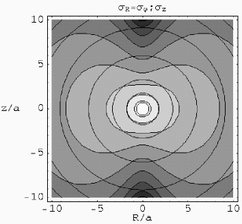
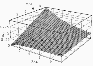
Figure 2: $R$ and $z$ dependence of the velocity dispersion ellipsoid (left) and anisotropy parameter $\beta=1-\sigma_{z}^{2}/\sigma_{R}^{2}$ (right) for the rotating model with DM and $V_{\mathrm{max}}=0.23v_{\mathrm{g}}$. In the left panel the contours of the $\sigma_{R}(=\sigma_{\varphi})$ component ($\sigma_{R}/v_{\mathrm{g}}$=0.325 to 0.125 with step=0.025 from inside) are plotted with different grey scales; the circular lines are the corresponding $\sigma_{z}$ contours.

2.3 Geometry and projected kinematics

As the galaxy intrinsic coordinate system we adopt a Cartesian coordinate system where the X-axis coincides with the direction of the line-of-sight and the Y-Z plane is the sky plane; the positive direction of the X-axis is towards the observer, while $V_{\mathrm{rad}}=-v_{x}$ is the radial velocity. In case of inclined systems, we adopt the conventional Euler matrix to identify the coordinate system X^′Y^′Z^′, where the X^′-axis is coincident with line-of-sight and the Y^′-Z^′ plane is the Sky plane. The three Euler angles are $\phi$, $\theta$, and $\psi$ (Goldstein, H. [1980]): when $\phi=\theta=\psi=0$, i.e. the edge-on case, the two coordinate systems XYZ and X^′Y^′Z^′ are coincident.
The projected rotation and velocity dispersion profiles are computed from the intrinsic profiles as follow. The projected moments of the radial velocities along the line-of-sight are given by the Abel integral

$$\langle V_{\mathrm{los}}^{(n)}\rangle=\frac{2}{I(\tau)}\int_{R}^{\infty}\overline{V_{\mathrm{rad}}^{n}}\frac{\rho r}{\sqrt{r^{2}-\tau^{2}}}dr$$ (13)

where $\tau$ is the distance from the galactic center along a fixed direction on the sky plane, $I(\tau)$ is the projected density, and $\overline{V_{\mathrm{rad}}^{n}}$ is the $n$-th moment of the radial velocity in each volume element along the line-of-sight. When we consider inclined systems, we have $V_{\mathrm{rad}}=-v_{x}^{\prime}=(a_{11}v_{x}+a_{12}v_{y}+a_{13}v_{z})$ in Eq. (13) where $a_{ij}$ are the elements of the Euler matrix. $V_{\mathrm{rad}}$ can be expressed in terms of the cylindrical velocity components:

$$v_{x} = v_{R}\cos\varphi~{}-~{}v_{\varphi}\sin\varphi$$

$$v_{y} = v_{R}\sin\varphi~{}+~{}v_{\varphi}\cos\varphi$$ (14)

$$v_{z} = v_{z}$$

where $\varphi$ is the conventional azimuthal angle in spherical and cylindrical coordinate systems. Then, $V_{\mathrm{rad}}=-(c_{1}v_{R}+c_{2}v_{\varphi}+c_{3}v_{z})$ where

$$c_{1} = a_{11}\cos\varphi+a_{12}\sin\varphi$$

$$c_{2} = -a_{11}\sin\varphi+a_{12}\cos\varphi$$ (15)

$$c_{2} = a_{13}.$$

When Eqs. (2.3) and (2.3) are substituted in Eq. (13), we derive the projected kinematics along the line-of-sight.
The rotation curve expected from the model at equilibrium is given by $\langle V_{\mathrm{los}}(\tau)\rangle$, and the velocity dispersion profile is given by $\sigma_{\mathrm{V}}^{2}=\langle V_{\mathrm{los}}^{2}(\tau)\rangle-\langle V_{\mathrm{los}}(\tau)\rangle^{2}$.

3 The simulated discrete radial velocity fields (SDRVF)

The dynamical state of a galactic system is described by its phase space distribution function (DF). With a functional form for the density distribution and gravitational potential, it is possible to determine the DF via the Eddington formula (Binney & Tremaine [1987]) for spherical systems.

In the case of the adopted Hernquist model, the Eddington formula is not so useful because its application required the use of special functions. To deal with the DF in a simple heuristic way, we adopt a factorised form

$$f({\bf r},{\bf v})=\rho({\bf r})F({\bf r},{\bf v})$$ (16)

where $\rho({\bf r})$ is the mass density distribution given by the model and $F({\bf r,v})$ is the velocity distribution depending on the position, ${\bf r}$, via its moments.

The observed distribution of radial velocity profiles in early-type galaxies are Gaussian, with maximum deviation of 10% (Winsall & Freeman [1993]; Bender et al. [1994]). In our modeling we will assume a velocity distribution given by the product of three Gaussian functions, although some anisotropy is implied by the assumed intrinsic cylindrical rotation. We write the velocity distribution as

$$F({\bf r},{\bf v})=F_{R}({\bf r},v_{R})F_{\varphi}({\bf r},v_{\varphi})F_{z}({\bf r},v_{z})$$ (17)

where

$$F_{i}({\bf r},v_{i})=\frac{1}{\sqrt{2\pi}\sigma_{i}({\bf r})}\exp\left[-\frac{(v_{i}-V_{i}({\bf r}))^{2}}{2\sigma_{i}^{2}({\bf r})}\right];~{}i=R,\varphi,z$$ (18)

and $F_{R}$, $F_{\varphi}$, $F_{z}$ are the normal distributions along the directions of the principal axes of the velocity ellipsoid. For each Gaussian, the mean value $V_{i}$ represents the mean motion and the standard deviation $\sigma_{i}$ is the diagonal element of the velocity ellipsoid in the same direction, both evaluated at position ${\bf r}$ ⁽⁾.

We consider both non-rotating and rotating systems: once the rotation velocity structure is assigned, we solve the Jeans equations for the given density distribution and obtain the velocity dispersion ellipsoid, plus the related projected velocity dispersion profiles. In rotating systems, the velocity distribution is given by Eq. (18), setting $V_{i}=v_{\mathrm{rot}}$ as in Eq. (8) and $\sigma_{i}$ as solutions of the Jeans equations Eqs.(11), (12); in non-rotating system, $V_{i}=0$ and $\sigma_{i}$ is given by Eq. (7)

We now generate a sample of discrete test particle from the mass density distribution $\rho({\bf r})$ and the distribution function $F({\bf r},{\bf v})$ as follows:

1. we randomly extract from $\rho({\bf r})$ the spherical coordinates $(r,\theta,\varphi)$ for each star and check that the corresponding projected radius $R$ is greater than $R_{\mathrm{lim}}$ (see Sect. 2),

2. from the velocity distribution $F({\bf r},{\bf v})$ we randomly extract the three velocity components $(v_{R},v_{\varphi},v_{z})$ at the position ${\bf r}$ of each star.

Once the 3D velocity field is obtained, we project it on the sky plane. The next step is to simulate a measurement of this two-dimensional velocity field: 1) we assume a typical measurement error for low to medium dispersion multi-object spectroscopy ($\sigma_{\mathrm{mea}}\sim$ 70 km/s = 0.08$v_{\mathrm{g}}$, see footnote 1), with a normal distribution; 2) the observed radial velocity measurement is obtained by a random extraction from a Gaussian, whose average is the $v_{\mathrm{rad}}$ value obtained for a single PN and standard deviation $\sigma_{\mathrm{mea}}$.
In this way we obtain a simulated discrete radial velocity field, $V_{\mathrm{obs}}(X,Y)$, from which the kinematical information is extracted.

4 Standard analysis procedure

From our simulated systems we want to estimate the kinematical quantities without using our knowledge of the intrinsic dynamics of our system. Therefore we apply to the simulated data a procedure similar to those adopted in the analysis of the small samples of discrete radial velocity fields of observed PNe (eg Arnaboldi et al. [1994], [1996], [1998]). In this procedure, we fit some simple three-parameter functions to our simulated data V${}_{\mathrm{obs}}(X,Y)$. We do this to see how misleading these fits can be if the real rotation fields have the form of Eq. (8). We perform a last-squares fit to the V${}_{\mathrm{obs}}(X,Y)$ using:

1. a bilinear function (hereafter BF)

   $$v_{\mathrm{rad}}=a+bX+cY$$ (19)

   where $X,\,Y$ are Cartesian coordinates of the PNe (typically in CCD coordinates) and $a$, $b$, $c$ are parameters to be determined by fitting Eq. (19) to the data. These parameters are used to determine the systemic velocity, direction of the axis of maximum velocity gradient, $Z1$, and modulus of the velocity gradient. This linear velocity field is equivalent to a solid body rotation of the form $v_{\mathrm{rad}}=v_{\mathrm{sys}}+\omega r\cos(\phi-\phi_{*})$ where $v_{\mathrm{sys}}$ is the systemic velocity, $\omega$ is the angular velocity, $\phi$ is the angle from the kinematic major axis, and $\phi_{*}$, the P.A. of the $Z1$ axis.

2. a flat rotation curve (hereafter FC)

   $$v_{\mathrm{rad}}=v_{\mathrm{sys}}+v_{*}\cos(\phi-\phi_{*})$$ (20)

   where $v_{\mathrm{sys}}$ and $\phi_{*}$ are the same quantities as in the BF, and $v_{*}$ is the amplitude of the flat rotation curve.

The residual field, $\Delta v$, is computed as the difference between V_obs and the interpolated radial fields from the fits. The residual fields obviously depend on the adopted fit (BF or FC). Furthermore we assume point-symmetry to the galaxy center for the simulated samples. Therefore to every velocity $v$ at position ($X,Y$) on the sky plane, there is a corresponding velocity $-v$ at position ($-X,-Y$). Hereafter we will refer to a symmetrized velocity field when we consider a sample generated on one side of the galaxy by adding the symmetric points generated by test particles on the other side.

5 Simulations

In Table 1 we summarise the set of parameters used in our models to generate the SDRVFs. Models with $V_{\mathrm{max}}$ up to 0.23$v_{\mathrm{g}}$ are physical, i.e. they have velocity dispersion ellipsoid components which are positive everywhere, while for $V_{\mathrm{max}}>0.23v_{\mathrm{g}}$ the $\sigma_{R}=\sigma_{\phi}$ components become negative for large $z$. However, we have kept these models because they have physical solutions near the equatorial plane, where the investigation of the kinematical observables (rotation velocity and velocity dispersion profiles) is often focussed.

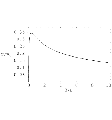
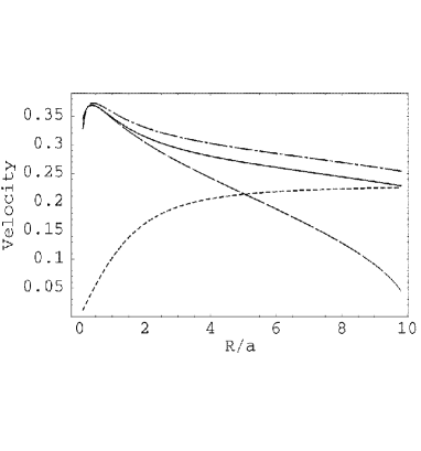
Figure 3: Here we show the solutions of the Jeans equations (Eqs. 11 and 12) as functions of distance from the center (R=$r$, $z$). Left: isotropic non-rotating system without DM. Right: rotating equilibrium model with DM and $V_{\mathrm{max}}=0.23v_{\mathrm{g}}$ (see Table 1); the $\sigma_{R}=\sigma_{\varphi}$ component is drawn as solid line on the equatorial plane and as long-dashed line along the rotation axis, while the $\sigma_{z}$ component is the dash-dotted line. The rotation velocity on the equatorial plane is also plotted, as short-dashed line.

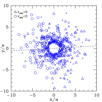
Figure 4: Left: a typical SDRVF obtained for a sample size of 500 PNe and the equilibrium model with DM and cylindrical rotation (inclination angles: 0:0:0). The dashed line is the line of the maximum gradient (computed with the bilinear fit). Right: the PNe number density (histogram) is compared with the surface brightness of the simulated system (solid line). The incompleteness of the sample is evident in the inner regions.

The solutions of the Jeans equations are shown in Fig. 3 for the system with $V_{\mathrm{max}}=0.23v_{\mathrm{g}}$ and for the non-rotating system. For our models we produce samples with 50, 150 and 500 PNe. For a given sample size, a fixed mass density model, a particular set of values for the rotation velocity (as given in Table 1) and inclination of the system, we produce 100 realisations of the radial velocity fields as described in Sect. 3. Fig. 4 shows a view of the the radial velocity field and the projected number density distribution obtained for a sample of 500 PNe for a rotating simulated system with $V_{\mathrm{max}}=0.23v_{\mathrm{g}}$ (see Table 1) seen edge-on. The comparison with the luminous matter projected density distribution shows the expected incompleteness effect in the generated PNe sample towards the center of the mass distribution. When computing the expected model quantities from Eq. (13), we take this selection effect into account, using the spatial and projected density profile obtained from a sample of 50 000 objects.

Table 1: Parameter values for the dynamical models which are used to generate the 2-D discrete radial velocity samples. The $a$ and $M_{\mathrm{l}}$ parameters are common to the self-consistent non-rotating and dark matter rotating systems. Here we adopt different values for the rotation vs. velocity dispersion so that any bias effects caused by the assumed functional form of the rotation field can be investigated. We refer to Sect. 5 for a detailed discussion. In parentheses we show the $v/\sigma$ value at $R=10a$.

Dynamical and kinematical parameters
$a$	1
$M_{\mathrm{l}}$	1
$d$	10$a$
$M_{\mathrm{d}}$	7.7$M_{\mathrm{l}}$
$r_{\mathrm{v}}$	2$a$
	0.35 $v_{\mathrm{g}}$ ($v/\sigma$=1.8)
	0.30 $v_{\mathrm{g}}$ (1.4)
$V_{\mathrm{max}}$	0.23 $v_{\mathrm{g}}$ (1.0)
	0.20 $v_{\mathrm{g}}$ (0.8)
	0.15 $v_{\mathrm{g}}$ (0.6)

5.1 Global kinematical quantities

To each SDRVF, we apply the analysis procedure described in Sect. 4 and derive the following kinematical quantities:

1. the velocity gradient, $gradV=\pm\sqrt{b^{2}+c^{2}}$ for the BF, with sign given by the sense of rotation;

2. the maximum rotation velocity (the $v_{*}$ parameter) for the FC;

3. the position angle of the maximum gradient, $\Phi_{Z1}=\arctan(c/b)$ for the BF, or $\Phi_{Z1}=\phi_{*}$ for the FC. Hereafter we refer to the axis of the maximum velocity gradient as $Z1$, with $Z2$ its perpendicular axis, i.e. the apparent rotation axis;

4. the systemic velocity $v_{\mathrm{sys}}=a$ for the BF and $v_{\mathrm{sys}}$ parameter from FC.

For each set of 100 simulations and a given sample size, we obtain the distribution of these global quantities, the related mean value and standard deviation of the sample (SD), which are then compared with the expected values to check for any presence of biases.

5.2 Projected kinematical quantities

To investigate the properties of our SDRVFs, we will implement a binning procedure, because similar strategies were applied to small observed radial velocity samples (like those for NGC 1399 and NGC 1316) and also in the case of NGC 5128 for which 433 radial velocities were available. Similar procedures are still adopted when using GCs data (eg Minniti et al. [1998]; Kissler-Patig et al. [1998]). In this framework we can also establish whether there are biases introduced by binning the observed radial velocity fields.

Once the line of maximum gradient is identified, the symmetrized velocity field is spatially binned along $Z1$, selecting particles within a strip along $Z1$. We have adopted strips having different width $dZ$ in order to check whether there was some dependence of the kinematical estimates on this parameter: see Table 3. The spatial binning is done in such a way that the number of particles in each bin is about 10 or more. We also do a radial binning by selecting PNe in radial annuli. This binning is usually done for radial velocity samples which are small, assuming spherical symmetry and isotropy. In our analysis of a given sample size, the radial and $Z1$ binning are fixed and maintained for all the 100 SDRVFs (the same binning is adopted for the $Z2$ axis because of spherical symmetry).

In the standard procedure, the mean values of the radial velocity sample in spatial bins along $Z1$ provides a measure of the rotation curve V_rot, while the velocity dispersion is obtained as SD in the same bins from the residual fields for the BF or FC. This gives an estimate of the observed dispersion $\sigma_{\mathrm{obs}}$ from which the projected velocity dispersion is obtained, using the independently determined measuring error $\sigma_{\mathrm{mea}}$, as $\sigma_{\mathrm{V}}=\sqrt{\sigma_{\mathrm{obs}}^{2}-\sigma_{\mathrm{mea}}^{2}}$. This velocity dispersion obviously depends on the adopted functional form of the rotation field. For comparison, we also estimated the velocity dispersion independently of the adopted rotation field, as the SD of the velocities from the mean radial velocity in each bin. Hereafter we refer to these estimates as NFP (no-fit procedure). We associate to each value of mean radial velocity V_rot an error given by $\delta V_{\mathrm{rot}}=SD/\sqrt{N}$ and to $\sigma_{\mathrm{obs}}$ an error $\delta\sigma_{\mathrm{obs}}=SD/\sqrt{2N}$. The behavior of $V_{\mathrm{obs}}$, $\sigma_{\mathrm{V}}$ and their relative errors from 100 simulations allow us to estimate the precision of any observable for a given sample size.

6 Results

6.1 Estimates of Kinematical Parameters

In Table 2 we list the results from our fits for the rotating model seen from three different line-of-sights (as identified by the Euler angles). For each set of simulations and fits, Table 2 shows the expected and estimated values of the kinematical parameters. The systemic velocity, $V_{\mathrm{sys}}$, and the P.A. of the maximum velocity gradient, $\Phi_{Z1}$, are well estimated from the fits of a simple three-parameter function. They are consistent with the expected model values at the 95% confidence level, for the potential with and without dark matter, and for both functions (BF and FC) that were fit to the velocity fields. We note the importance of an accurate estimate for the position angle $\Phi_{Z1}$, because $\Phi_{Z1}$ is then used in the analysis of the projected kinematics. Systematic errors on $\Phi_{Z1}$ produce systematic errors on the projected kinematics.

The velocity gradient and maximum rotation velocity estimates are systematically incorrect when they are obtained from the wrong simple function. In the case of cylindrical rotation, the BF can produce a large over-estimate of the velocity gradient (up to about 100%) while the FC (which is closer to being the correct functional form for the rotation adopted in the model) gives only a small under-estimate. The reason is clear from examination of Fig. 5

Figure 5: Biases in the maximum gradient and maximum rotation velocity. The intrinsic rotation curve from the model (curved solid line, $V_{\mathrm{max}}=0.3v_{\mathrm{g}}$, see Table 1) is compared with the bilinear fit (left), the flat-curve fit (right) and the mean values in bins (filled points) obtained on 100 simulations. The parameters of the fitted functions are the averages from the same 100 simulations: straight solid lines show the BF (left) and FC (right) fits, and dot-dashed lines are the $\pm$SD lines about the fits. Quoted errors about the points are the SDs of the distribution of estimates in each bin. The dashed vertical line indicates the inner limiting radius, $R_{\mathrm{lim}}$.

Table 2: Results obtained for the equilibrium model with DM and flat cylindrical rotation: behavior from 100 SDRVFs. Square parentheses: the unit in which the quantities are given; round parentheses: the expected values. Quoted errors are SDs of the derived quantities.

Model with DM - Rotation Curve of Equation (9)
Proced.	BF			FC
Inclin.	$\phi=0$ $\theta=0$ $\psi=0$
$N^{o}$ PNe	$\Phi_{Z1}$[rad](0)	gradV$[v_{\mathrm{g}}/a]$ (0.023)	$V_{\mathrm{sys}}[v_{\mathrm{g}}]$ (0)	$\Phi_{Z1}$[rad](0)	$v_{*}[v_{\mathrm{g}}]$ (0.23)	$V_{\mathrm{sys}}[v_{\mathrm{g}}]$ (0)
500	0.00$\pm$0.08	0.046$\pm$0.005	0.002$\pm$0.013	-0.01$\pm$0.09	0.182$\pm$0.019	0.000$\pm$0.014
150	-0.06$\pm$0.22	0.045$\pm$0.010	0.01$\pm$0.02	0.00$\pm$0.23	0.18$\pm$0.04	0.00$\pm$0.02
50	0.0$\pm$0.3	0.048$\pm$0.015	0.0$\pm$0.04	0.0$\pm$0.3	0.18$\pm$0.06	0.00$\pm$0.04
Inclin.	$\phi=-45$ $\theta=-45$ $\psi=-45$
$N^{o}$ PNe	$\Phi_{Z1}$[rad] (0.62)	gradV$[v_{\mathrm{g}}/a]$ (0.021)	$V_{\mathrm{sys}}[v_{\mathrm{g}}]$ (0)	$\Phi_{Z1}$[rad](0.62)	$v_{*}[v_{\mathrm{g}}/a]$ (0.21)	$V_{\mathrm{sys}}[v_{\mathrm{g}}]$ (0)
500	0.61$\pm$0.12	0.039$\pm$0.005	-0.002$\pm$0.013	0.62$\pm$0.12	0.155$\pm$0.022	-0.003$\pm$0.014
150	0.61$\pm$0.23	0.040$\pm$0.009	0.00$\pm$0.02	0.61$\pm$0.23	0.16$\pm$0.04	-0.01$\pm$0.02
50	0.5$\pm$0.4	0.041$\pm$0.013	0.00$\pm$0.04	0.5$\pm$0.3	0.16$\pm$0.05	0.00$\pm$0.04
Inclin.	$\phi=90$ $\theta=90$ $\psi=30$
$N^{o}$ PNe	$\Phi_{Z1}$[rad] (indet.)	gradV$[v_{\mathrm{g}}/a]$ (0)	$V_{\mathrm{sys}}[v_{\mathrm{g}}]$ (0)	$\Phi_{Z1}$[rad](indet.)	$v_{*}[v_{\mathrm{g}}/a]$ (0)	$V_{\mathrm{sys}}[v_{\mathrm{g}}]$ (0)
500	0.13$\pm$0.99	-0.001$\pm$0.006	-0.002$\pm$0.014	0.14$\pm$0.67	0.01$\pm$0.01	-0.002$\pm$0.014
150	0.01$\pm$0.89	0.001$\pm$0.013	0.00$\pm$0.03	0.06$\pm$0.62	0.02$\pm$0.03	0.00$\pm$0.03
50	0.09$\pm$ 0.98	0.000$\pm$0.022	0.00$\pm$0.05	0.18$\pm$0.65	0.04$\pm$0.04	0.00$\pm$0.05

6.2 Estimates of kinematical quantities

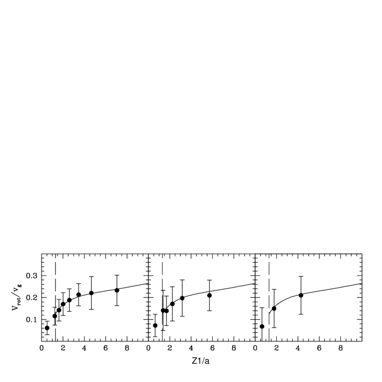
Figure 10: Velocity rotation curves for the systems with $V_{\mathrm{max}}=0.30v_{9}$. Top: Z1 axis (edge-on); center: Z2 axis (edge-on); bottom: Z1 axis (LOS: -45,-45,-45). The vertical long dashed line indicates $R_{\mathrm{lim}}$, full points are the mean values obtained on 100 simulations, solid line is the expected velocity rotation. Left: 500 PNe; center: 150 PNe; right: 50 PNe.

Figure 11: Velocity rotation curves along Z1 and Z2 for the systems with $V_{\mathrm{max}}=0.30v_{9}$, face-on case. Empty circles are the mean values obtained on 100 simulations along Z1, empty squares are the mean values along Z2, solid line is the expected velocity rotation. Left: 500 PNe; center: 150 PNe; right: 50 PNe.

Rotation velocity curves The mean velocity rotation curves evaluated from 100 SDRVFs for each given sample size follow the theoretical behaviour predicted by the models for every parameter choice (Fig. 11). Rotation along $Z2$ is everywhere consistent with the null rotation (Fig. 11).
In Figs 11 and 11 we show the results obtained considering the inclined system: the rotation velocity is decreased by the expected $\sin i$ factor, where $i$ is the angle between the line-of-sight and rotation axis given by a particular set of Euler angles. For face-on model, no-rotation is found, as expected (Fig. 11).
 
Velocity dispersion profiles along the Z1 and Z2 axes - The inferred velocity dispersion profiles are of particular interest because they allow the evaluation of the mass distribution via inversion of the Jeans equations. When the velocity dispersion profiles are computed from the residual velocity fields, they can be affected by biases resulting from the simple functional forms used to fit the discrete radial velocity sample.

When the equilibrium model with cylindrical rotation is compared with the results for larger samples (eg 150 and 500), the velocity dispersion profiles obtained from the BF residuals along the Z1 axis show a small but visible over-estimate of $\sigma_{\mathrm{V}}$ in the outer bins relative to the expected values from the model. Better agreement is found using the FC (see Fig. 14). This happens because, along the maximum gradient axis, the flat rotation curve gives a better description for the rotational structure of the equilibrium model under study, whose rotation becomes flat at large distances from the center along the $Z1$-direction.

Figure 6: Biases from BF in dark matter systems: points represent the relative deviation of the velocity dispersion determined in the last bin along Z1 with respect the “true” value expected from model. Error bars take in to account errors on the estimates on 100 simulations. The behavior shown by the residuals indicates that higher rotation in the model causes the bilinear fit to introduce a larger bias in the estimated velocity dispersion profile. The vertical arrow shows the bias in the velocity dispersion estimate, for the model with $V_{\mathrm{max}}=0.30v_{\mathrm{g}}$ (see also Figure 14).

We find a clear and expected correlation of this bias with the $v/\sigma$ ratio. In the last bin along $Z1$, we compute the difference $\Delta\sigma=\sigma_{\mathrm{V}}-\sigma_{\mathrm{mod}}$, between the dispersion values estimated from BF ($\sigma_{\mathrm{V}}$), and the expected dispersion from the models ($\sigma_{\mathrm{mod}}$), for different values of $(v/\sigma)_{\mathrm{obs}}=V_{\mathrm{rot}}/\sigma_{\mathrm{V}}$ values in the last bin (obtained by varying the $V_{*}$ parameter in the rotating models). The results for 500 PNe are shown in Fig. 6. The bias in the velocity dispersion in the last bins is an increasing function of the $(v/\sigma)_{\mathrm{obs}}$ ratio: larger rotation causes the bilinear fit to introduce a larger overestimate of the velocity dispersion profile.

As mentioned earlier, for small radial velocity samples this kind of bias is associated not only with our simple parametric fits but also with more sophisticated non-parametric analyses. When there are fewer data points, the non-parametric algorithms with their inherent smoothing effectively fit a plane through the data, so the velocity dispersion profiles derived from the residual fields do suffer from similar biases as the one we are investigating in the case of a simple bilinear fit.

In general, for all sample sizes, the velocity dispersion estimates along the Z1 axis obtained using the NFP are in better agreement with the expected ones. The estimates along Z2 axis are not affected by this bias: in Fig. 14 the estimates from BF and FC are in agreement with the model, while NFP systematically overestimates the velocity dispersion values in the bins. This effect depends on the strip dimension adopted to select particles along the rotational axis: the expected profile is computed along the Z2-axis, while the estimates are obtained on bins and their widths include regions where the velocity dispersion is larger (see Fig. 2). On average, they trace a larger dispersion and this causes an overestimate. On the other hand, the different fit procedures subtract a gradient in these bins, and produce a lower dispersion. In Fig. 14, the estimates with the smallest dZ2, adopted for the different samples, show the magnitude of this effect. Smaller dZ2 reduce the overestimate but the errors are larger. All these features are found for the inclined systems too, as shown in Fig. 15. Here the profiles follow those of the edge-on case, but the amount of bias due to the fitting procedure is smaller because the $(v/\sigma)_{\mathrm{obs}}=V_{\mathrm{rot}}/\sigma_{\mathrm{V}}$ ratio is lower. In the face-on case, no biases are found as in case of non-rotating self consistent model (Fig. 13).
 
Velocity dispersion profiles from radial bins - When we derive the velocity dispersion profiles from the residual velocity field (either from BF or FC) in radial annuli, they show effects from the azimuthal dependence of the intrinsic velocity dispersion ellipsoid. Those profiles derived either from BF or FC have a behavior which is intermediate between those expected from the model along $Z1$ and $Z2$ (Figs. 13 and 17) for the edge-on and the inclined cases. In the face-on case (Fig. 17), no azimuthal dependence is expected or seen (see Fig. 2). On the other hand, the velocity dispersion profiles obtained with radial binning and NFP show a strong overestimate of the velocity dispersion values due to the cylindrical structure of the intrinsic velocity field.

7 Sampling errors

The sampling errors are related to the size of a given sample, and affect the accuracy of the kinematical quantities we are trying to estimate. They are important because they often dominate the error budget of the estimated mass and angular momentum estimates in halos of galaxies. In this work, for given sample sizes, we simulated 100 realisations of the radial velocity field, from which we derived the distribution of the kinematical measurements. We then compare the uncertainty estimated (internally) from single measurements of a kinematical observable with the uncertainty from the distribution of that observable from 100 simulations. This allows us to check i) whether the statistical errors are evaluated in a realistic way for single measurements and ii) study the behavior of the sampling errors and the precisions based on their actual distributions.

Table 3: Average relative precision considering all bins and models: RB are radial bins, $dZ_{\mathrm{min}}$ and $dZ_{\mathrm{max}}$ are the minimum and maximum width of the strips adopted along the Z-axes. In parentheses we indicate the mean number of PNe selected with our choice of the bin dimensions.

Relative errors on velocity dispersion
No PNe	RB $(\overline{N})$	$dZ_{\mathrm{min}}~{}(\overline{N})$	$dZ_{\mathrm{max}}~{}(\overline{N})$
500	0.106$\pm$0.001 (55)	0.211$\pm$0.015 (23)	0.164$\pm$0.006 (34)
150	0.188$\pm$0.005 (20)	0.310$\pm$0.015 (9)	0.233$\pm$0.007 (14)
50	0.238$\pm$0.016 (15)	0.38$\pm$0.03 (8)	0.251$\pm$0.015 (12)

Table 4: Average relative precision in the last bin: RB are radial bins, $dZ_{\mathrm{min}}$ and $dZ_{\mathrm{max}}$ are the minimum and maximum width of the strips adopted along the Z-axes. In parentheses we indicate the mean number of PNe selected with our choice of the bin dimensions.

Relative errors on velocity dispersion in last bin
No PNe	RB$~{}(\overline{N})$	$dZ_{\mathrm{min}}~{}(\overline{N})$	$dZ_{\mathrm{max}}~{}(\overline{N})$
500	0.12$\pm$0.02 (48)	0.32$\pm$0.03 (8.5)	0.24$\pm$0.03 (12.5)
150	0.21$\pm$0.02 (17)	0.37$\pm$0.04 (8)	0.25$\pm$0.03 (13)
50	0.28$\pm$0.02 (11)	0.47$\pm$0.08 (7)	0.29$\pm$0.03 (11)

7.1 Errors on the velocity dispersion

For all models and velocity dispersion profiles, we compute the average of the relative errors on 100 simulations in all bins (for which the PNe number density is complete) for a given sample size. We consider this to be indicative of the precision for the velocity dispersion. We do this for the spatial binning along $Z1$, $Z2$, and for radial bins. The results are shown in Table  3.

Figure 7: Left: behavior of the relative errors on the velocity dispersion with respect the mean number density in the last bin (full points) and in two more bins (see footnote 9) on all the simulation done for all the models. Solid line is a fit to the data points using the function $A/\sqrt{\overline{N}}+B$. Right: correlations between relative errors for the rotation velocity and $(v/\sigma)_{\mathrm{obs}}$ in the last bin. Here different symbols are adopted for different models, sample sizes and bin dimensions. They fill in the region identified by the fitted function for the maximum mean sample, $\overline{N}$=13, and the minimum one, $\overline{N}$=7, per bin used in our simulations. Dash-dotted lines are for intermediate number samples.

The average relative errors depend only on sample size and are quite independent on the fitting function, inclination, and the mass and rotation models. If we consider the estimates along the Z-axes, for a sample size of 500 test particles the precision on velocity dispersion is 16%, for 150 test particles it is 23%, and for a sample of 50 test particles it is 25%. Higher precisions (10% for 500 PNe, 19% for 150 PNe, 24% for 50 PNe) are found if we consider the estimates in radial bins (where the whole sample size is used). The mean number of particles related to these estimates are shown in Table 3.

The results for the last bins are shown in Table 4. The relative errors are plotted in Fig. 7 against $\overline{N}$, showing a pseudo-Gaussian behavior. The distribution is reproduced by the function $A/\sqrt{\overline{N}}+B$, with best fit parameters, A=$0.94\pm 0.06$ and B=$-0.01\pm 0.02$. If $\delta\sigma_{\mathrm{V}}/\sigma_{\mathrm{V}}=1/\sqrt{2\overline{N}}$, the B and A values should be zero and $1/\sqrt{2}=0.71$ respectively. Our estimate for B is consistent with zero. We find A=0.94$>$0.71 because by definition $\delta\sigma_{\mathrm{p}}/\sigma_{\mathrm{p}}=1/\sqrt{2\overline{N}}$ and $\sigma_{\mathrm{V}}^{2}=\sigma_{\mathrm{p}}^{2}-\sigma_{\mathrm{mea}}^{2}$ so

$$\frac{\delta\sigma_{\mathrm{V}}}{\sigma_{\mathrm{V}}}=\frac{1}{1-\sigma_{\mathrm{mea}}^{2}/\sigma_{\mathrm{p}}^{2}}\frac{\delta\sigma_{\mathrm{p}}}{\sigma_{\mathrm{p}}}=C_{\sigma}\frac{\delta\sigma_{\mathrm{p}}}{\sigma_{\mathrm{p}}}>\frac{\delta\sigma_{\mathrm{p}}}{\sigma_{\mathrm{p}}}=\frac{1}{\sqrt{2\overline{N}}}.$$ (21)

For a typical $\sigma_{\mathrm{mea}}/\sigma_{\mathrm{p}}$=0.4 in last bins, $C_{\sigma}$=1.2 and the expected value for the A parameter is A=$C_{\sigma}/\sqrt{2}$=1.2$\times$0.71=0.85. Furthermore $\sigma_{\mathrm{V}}=(\sigma_{\mathrm{p}}^{2}-\sigma_{\mathrm{mea}}^{2})^{1/2}$ is not a Gaussian variable, as we do not have a linear relation between $\sigma_{\mathrm{V}}$ and $\sigma_{\mathrm{p}}$, so this causes an overestimate when $\sigma_{\mathrm{V}}$ is computed as a Gaussian quantity.
Finally, the computed value for A accounts for an average behavior of the velocity dispersion relative errors on a wide range of models and it can be considered as an upper limit for the relative errors, once given the number sample in bins.
We have then compared the precisions on a single measurement, obtained as in Eq. (21), with those expected from the related distribution on 100 simulations and found that they are consistent within the errors.

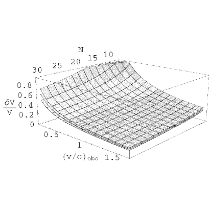
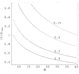
Figure 8: Precisions on rotation velocity. Left: behaviour of the generalised relative errors as function of $\overline{N}$ and $(v/\sigma)_{\mathrm{obs}}$, with the $\pm$SD surfaces which are computed from the errors on the $a$ and $b$-parameters. Right: 15%, 20%, 30%, 40% contours of the generalised relative errors.

7.2 Errors on the rotation velocity

We focus our analysis on the last spatial bin of the rotation velocity curves, because the outer regions are those for which we wish to derive the mass and angular momentum estimate. The statistical errors for the velocity rotation measurements depend on the adopted model and bin dimensions. The bin dimension determines the number statistics and involves the velocity range over which we compute the average rotation for a selected sample. The mass and rotation model determine the dispersion profile which is needed for the equilibrium, and this velocity dispersion enters in to the error budget of the rotation measurement. In fact, using the definition of errors on the rotation velocity, we have

$$\frac{\delta V_{\mathrm{rot}}}{V_{\mathrm{rot}}}=\frac{\sigma_{\mathrm{p}}}{\sqrt{\overline{N}}}\frac{1}{V_{\mathrm{rot}}}$$ (22)

where $\sigma_{\mathrm{p}}=\sigma_{\mathrm{V}}\sqrt{1+\sigma_{\mathrm{mea}}^{2}/\sigma_{\mathrm{V}}^{2}}=C_{\mathrm{V}}\sigma_{\mathrm{V}}$ and

$$\frac{\delta V_{\mathrm{rot}}}{V_{\mathrm{rot}}}=\frac{C_{\mathrm{V}}}{\sqrt{\overline{N}}}\frac{\sigma_{\mathrm{V}}}{V_{\mathrm{rot}}}=\frac{C_{\mathrm{V}}}{\sqrt{\overline{N}}}\left(\frac{v}{\sigma}\right)^{-1}_{\mathrm{obs}}.$$ (23)

Table 5: Here we list the set of parameter values for the fits displayed in Fig. 7 (right panel).

Parameters in $\delta v/v$ fit
$\overline{N}$	$A$	$B$
29	0.185 $\pm$0.019	0.00$\pm$0.03
14	0.27 $\pm$0.05	0.00$\pm$0.07
13	0.28 $\pm$0.02	0.02$\pm$0.03
12.5	0.29 $\pm$0.02	0.015$\pm$0.020
11	0.30 $\pm$0.02	0.05$\pm$0.03
8.5	0.38 $\pm$0.03	0.03$\pm$0.04
8	0.39 $\pm$0.04	0.02$\pm$0.05
7	0.50 $\pm$0.04	-0.02$\pm$0.06

Here we want to check this dependence. For a fixed $\overline{N}$ (i.e. the mean number of particles in the last bin), one expects the relative errors to be reproduced by the following function

$$\frac{\delta v}{v}=A{(v/\sigma)_{\mathrm{obs}}}^{-1}+B.$$ (24)

In Fig. 7 the best-fit for different $\overline{N}$, as in Table 5 are shown. For these curves, B is always consistent with zero, while, from Eqs. (23) and (24), we expect A=$C_{\mathrm{V}}/\sqrt{\overline{N}}$ and $C_{\mathrm{V}}$=1.08, for a typical $\sigma_{\mathrm{mea}}/\sigma_{\mathrm{V}}$=0.4 in the last bins. To test this dependence, the A parameter obtained for the different error profiles in Fig. 7 is interpolated with the function $a/\sqrt{\overline{N}}+b$; the best fit is for a=1.15$\pm$0.10 and b=-0.02$\pm$0.03, in agreement with the expected behavior.

All these results were obtained for a wide range of models, so they can be generalised and used to estimate the sample size needed to reach a targeted precision of the observed kinematical quantities.

Once the kinematics is known from integrated light in the inner region of a galaxy system, we can estimate the minimum sample needed to reach a targeted precision in the outer regions, based on the inner $(v/\sigma_{\mathrm{obs}})$. In Fig. 8 we show the dependence of rotation velocity precisions based on the results in Fig. 7, as function of $(v/\sigma)_{\mathrm{obs}}$ and $\overline{N}$. In the same Figure, the contours for different precisions are shown. The results of this analysis indicate that 1) the relative errors on the rotation velocity computed from a single measurement are consistent with those expected from the distribution of 100 simulation, 2) the precision on the rotational velocity is correlated with the internal kinematics of real systems and 3) this correlation is quite general and can be used in feasibility studies, once we need to estimate exposure times and plan observing proposals to reach a given sample size, i.e. a targeted precision. For example, if one needs to reach an accuracy on $V_{\mathrm{rot}}$ of 20%, at least 30 PNe are needed in the last bin for systems were $(v/\sigma>1)$; to reach similar precision, larger samples are needed for systems with a lower value of $(v/\sigma)$.

8 Summary and conclusions

We have developed an algorithm to simulate real measurements of discrete radial velocity fields for a given mass model at equilibrium, using a simplified DF in a factorized form, and with different sample sizes. We use this algorithm to address two important questions when using discrete radial velocity fields as a tool to study the kinematics of the outer regions of elliptical galaxies:

1. Are the simple 3-parameter functional forms used to fit small sample of PNe radial velocities introducing biases on estimates of the kinematical quantities?

2. How does the precision of a kinematical estimate depend on the sample sizes, taking into account the rotation and inclination of the system under study?

The answers are the following:
1) A bilinear fit to a sample coming from a system with a rotation curve like that of Centaurus A (Eq. 8) does introduce a bias in the velocity dispersion profile at large radii. This problem is important and pervades more sophisticated non-parametric analyses. Any kind of smoothing algorithm applied to a small discrete sample of observed radial velocities, as in the study of NGC 1316 by Arnaboldi et al. ([1998]), is effectively fitting a more or less bilinear form to the data. Our simulations show that this is bound to introduce a bias in the estimate of the velocity dispersion profile derived from the residual field, in particular for highly rotating systems. A flat rotation curve, or a rotation curve profile derived from averaged data in bins along the line of maximum gradient, should be adopted to derive the best estimate for $\sigma$. Such a procedure was indeed used in the case of NGC 5128 (Hui et al. [1995]). The overestimate in $\sigma$ caused by fitting a plane can be up to 20% in $\sigma$, i.e. 40% in the total mass. This bias correlates with the $(v/\sigma)$ ratio, in the sense that higher rotation leads to stronger biases in $\sigma$. We also identified the most reliably estimated quantity derived when using these simple 3-parameter fields: the line of maximum gradient. This leads us to adopt the NFP, i.e. the analysis of the binned quantities along this P.A., as the best approach free of analysis-induced biases.
2) We have found that the precisions obtained on single measurements are consistent with those obtained from the simulated distributions. Moreover we have found a generalised relation between the precision one can obtain for the observables in the outer regions as function of sample size and inner kinematics. This empirical relation can be very extensively used to plan and estimate observing times to study the dynamics of the outer haloes of giant early type galaxies with multi slit spectrographs like FORS2 or VIMOS on VLT, or in slitless spectroscopy.

Appendix: the theoretical signal-noise ratio (SNR)

In our simulated velocity fields we introduce a cut-off in the projected PN density distribution determined by a inner limiting radius, at which the incompleteness of the observed PNe sample due to the bright continuum light in the central part of an E galaxy becomes significant. For a given luminosity profile, we consider all the PNe having magnitude $m=m_{\mathrm{lim}}$ which is the faintest magnitude in a PNLF for a complete sample, and we compute the SNR with respect to the galaxy background. We take a PN to be detected if it has a detected flux with SNR=9 (Ciardullo et al. [1987]). Considering a negligible read-out-noise and sky background distribution, the SNR is defined as follows

$$SNR=\frac{N_{5007}}{\sqrt{N_{5007}+N_{\mathrm{gal}}}}$$ (25)

where $N_{5007}$ are the photon counts detected for a single PN in the 5007 Å [OIII] line and $N_{\mathrm{gal}}$ are the photon counts from the continuum galaxy background. These quantities are related to the incoming fluxes as follows

$$N_{5007}=\frac{F_{5007}~{}t_{\mathrm{esp}}~{}S_{\mathrm{tel}}~{}\varepsilon}{E_{5007}}$$ (26)

where $F_{5007}$ is the flux received in the 5007 Å line, $t_{\mathrm{esp}}$ is the exposure time, $S_{\mathrm{tel}}$ is the telescope surface, $\varepsilon$ is the total efficiency (instrumental efficiency + atmosphere absorption), $E_{5007}$ is the energy of the photons at $\lambda=$5007 Å

$$N_{\mathrm{gal}}=\frac{F_{V}}{E_{V}}\Delta\lambda~{}t_{\mathrm{esp}}~{}S_{\mathrm{tel}}~{}\varepsilon~{}S_{\mathrm{sd}}\simeq\frac{F_{V}}{E_{5007}}\Delta\lambda~{}t_{\mathrm{esp}}~{}S_{\mathrm{tel}}~{}\varepsilon~{}S_{\mathrm{sd}}$$ (27)

where $F_{V}$ is the flux per unit area received by the continuum galaxy background in the V-band, $\Delta\lambda$ is the pass band of a typical narrow filter, and $S_{\mathrm{sd}}$ is the area of the seeing disk ($S_{\mathrm{sd}}=\pi(3*FWHM/2.356)^{2}$).
Substituting (26) and (27) in the relation (25), we find that

$$SNR=F_{5007}\sqrt{\frac{t_{\mathrm{esp}}~{}S_{\mathrm{tel}}~{}\varepsilon}{E_{5007}}}\frac{1}{\sqrt{F_{5007}+F_{\mathrm{V}}\Delta\lambda S_{\mathrm{sd}}}}$$ (28)

where

$$F_{\mathrm{V}}=10^{-0.4(8.3268\left(\frac{R}{R_{\mathrm{e}}}\right)^{1/4}+12.7532+\mu_{\mathrm{e}}-(B-V))}\\$$ (29)

and

$$F_{5007}=10^{-0.4(m_{\mathrm{lim}}+13.74)}$$ (30)

(Ciardullo et al. [1989]). In Fig. 9, we plot the $SNR$ for a 3.6m telescope, using $T_{\mathrm{esp}}=3$ hrs, $\Delta\lambda=$60 Å, FWHM=1.3^′′ and $\varepsilon$=0.5 and considering $m_{\mathrm{lim}}$=27.2 mag, $\mu_{\mathrm{e}}$=21.24 mag arcsec^-2 and B-V=0.1 which are the typical values for an E galaxy in Virgo Cluster (Caon et al. [1994]; McMillan et al. [1993]). The condition $SNR(R_{\mathrm{lim}})=9$ implies $R_{\mathrm{lim}}=0.7R_{\mathrm{e}}$.

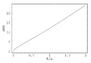
Figure 9: The R-coordinate dependence of the $SNR$ for our parameter choice.

Figure 12: Velocity dispersion profiles for non-rotating systems: model without DM. Full points are the mean values obtained on 100 simulations, solid line is the expected velocity dispersion profile. Top: 500 PNe;middle: 150 PNe; bottom: 50 PNe. Left: in radial bins; center: along Z1 axis; right: along Z2 axis.

Figure 13: Velocity dispersion profiles in radial bins: rotating model with DM and $V_{\mathrm{max}}=0.23v_{\mathrm{g}}$, edge-on case. Full points are the mean values obtained on 100 simulations, solid line is the expected velocity dispersion profile along the Z1-axis, dot-dashed line is the expected velocity dispersion profile along the Z2-axis. The estimates by the fitting procedures (BF and FC) show the azimuthal dependence while the NFP causes an overestimation of the velocity dispersion values. Top: 500 PNe; middle: 150 PNe, bottom: 50 PNe. Left: bilinear fit procedure; center: no-fit procedure; right: flat-curve procedure.

Figure 14: Velocity dispersion profiles for rotating model with DM along Z1 (upper panel, $V_{\mathrm{max}}=0.30v_{\mathrm{g}}$) and Z2 (lower panel, $V_{\mathrm{max}}=0.23v_{\mathrm{g}}$): edge-on case. Full points are the mean values obtained on 100 simulations, solid line is the expected velocity dispersion profile, empty squares are the estimates using $dZ_{\mathrm{min}}$. The bias introduced by the BF is indicated by the arrow (upper panel 500 PNe case; see also Fig. 6). In each panel: Top: 500 PNe; middle: 150 PNe;bottom: 50 PNe. Left: bilinear fit procedure; center: no-fit procedure; right: flat-curve procedure.

Figure 15: Velocity dispersion profiles for rotating model with DM along Z1 (upper panel, $V_{\mathrm{max}}=0.30v_{\mathrm{g}}$) and Z2 (lower panel, $V_{\mathrm{max}}=0.23v_{\mathrm{g}}$). LOS: -45:-45:-45. Symbols have the same meaning as in Fig. 14. The amount of the biases is negligible here because the $(v/\sigma)_{\mathrm{obs}}=V_{\mathrm{rot}}/\sigma_{\mathrm{V}}$ ratio is lower. In each panel: Top: 500 PNe; middle: 150 PNe;bottom: 50 PNe. Left: bilinear fit procedure; center: no-fit procedure; right: flat-curve procedure.

Figure 16: Velocity dispersion profiles in radial bins: rotating model with DM and $V_{\mathrm{max}}=0.23v_{\mathrm{g}}$. LOS: -45:-45:-45. Symbols have the same meaning as in Figure 13. Top: 500 PNe; bottom: 50 PNe. Left: bilinear fit procedure; center: no-fit procedure; right: flat-curve procedure.

Figure 17: Velocity dispersion profiles in radial bins: rotating model with DM and $V_{\mathrm{max}}=0.23v_{\mathrm{g}}$, face-on case. Here the expected velocity dispersion profile (solid line) has no azimuthal dependence and a perfect agreement is found with the estimates (filled squares). Top: 500 PNe;center: 150 PNe; bottom: 50 PNe. Left: bilinear fit procedure; center: no-fit procedure; right: flat-curve procedure.

References

- [1994] Arnaboldi, M., Freeman, K.C., Capaccioli, M., Ford, H., 1994, ESO Messenger 76, 40
- [1996] Arnaboldi, M., Freeman, K.C., Mendez, R., Capaccioli, M., Ciardullo, R., Ford, H., Gerhard, O., Hui, X., Jacoby, G.H., Kudritzki, R.P., Quinn, P.J., 1996, ApJ 472, 145
- [1998] Arnaboldi, M., Freeman, K.C., Gerhard, O., Matthias, M., Kudritzki, R.P., Mendez, R., Capaccioli, M., Ford, H., 1998, ApJ 507, 759
- [1995] Arnold, R., 1995, MNRAS 276, 293
- [1994] Bender, R., Saglia, R.P., Gerhard, O.E., 1994, MNRAS 269, 785
- [1987] Binney, J.J., & Tremaine, S., 1987, Galactic Dynamics, Princeton Series in Astrophysics
- [1994] Caon, N., Capaccioli, M., D’Onofrio, M., 1994, A&A 106, 199
- [1987] Ciardullo, R., Ford, H.C., Neill, J.D, Jacoby, G.H., Shafter, A.W., 1987, ApJ 318, 520
- [1989] Ciardullo, R., Jacoby, G.H., Ford, H.C., Neill, J.D., 1989, ApJ 339,53
- [1991] Ciardullo, R., Jacoby, G.H., Harris, W.E., 1991, ApJ 383, 487
- [1993] Ciardullo, R., Jacoby, G.H., Dejonghe, H.B., 1993, ApJ 414, 454
- [2000] Cohen, J.G., 2000, AJ 119, 162
- [1948] de Vaucouleurs, G., 1948, Ann. d’Astrophys. 11, 247
- [1992] Dopita, M.A., Jacoby, G.H., Vassiliadis, E., 1992, ApJ 389, 27
- [1996] Ford, H. C., Hui, X., Ciardullo, R., Jacoby, G. H., Freeman, K. C., 1996, ApJ 472, 145
- [1994] Grillmair, C.J., Freeman, K.C., Bicknell, G.V., Carter, D., Couch, W.J., Sommer-Larsen, J., Taylor, K., 1994, ApJ 422, 9
- [1980] Goldstein, H., 1980, Classical Mechanics, 2nd ed. Reading, Penn.: Addison-Wesley.
- [1988] Harris, W., 1988, IAU Symposium 126, 237
- [1990] Hernquist, L., 1990, ApJ 356, 359
- [1995] Hui, X., Ford, H., Freeman, K.C., Dopita, M.A., 1995, ApJ 449, 592
- [1998] Kissler-Patig, M., Forbes, D.A., Minniti, D., 1998, MNRAS 298, 1123
- [1960] Lynden-Bell, D., 1960, MNRAS 120, 204
- [1993] McMillan, R., Ciardullo, R., Jacoby, G.H., 1993, ApJ 416, 62
- [1998] Minniti, D., Kissler-Patig, M., Goudfrooij, P., Meylan, G., 1998, AJ 115, 121
- [1990] Mould, J.R., Oke, J.B., de Zeew, P.T., Nemec, J.M., 1990, AJ 99, 1823
- [1987] Nolthenius, R., & Ford, H., 1987, ApJ 317, 62
- [1988] Sharples, R., 1988, IAU Symposium 126, 545
- [1995] Tremblay, B., Merritt, D., Williams, T.B., 1995, ApJL 443, 5
- [1993] Winsall, M.L., & Freeman, K.C., 1993, A&A 268, 443