Cosmological Hydrogen Reionization with Three Dimensional Radiative Transfer

Abstract

We present new calculations of the inhomogeneous process of cosmological reionization by following the radiative transfer carefully in pre-computed hydrodynamical simulations of galaxy formation. These new computations represent an important step on the way towards fully self-consistent and adaptive calculations which will eventually cover the enormous range of scales from sizes of individual mini-halos to the mean free path of ionizing photons in the post-overlap Universe. The goal of such simulations is to include enough realistic physics to accurately model the formation of early structures and the end of the ‘dark ages’. Our new calculations demonstrate that the process by which the ionized regions percolate the Universe is complex, and that the idea of voids being ionized before overdense regions is too simplistic. It seems that observational information pertaining to the reionization epoch may now be in our grasp, through the detection of Gunn-Peterson troughs at $z\sim 6$. If so, then the comparison of information from many lines of sight with simulations such as ours may allow us to disentangle details of the ionization history and trace the early formation of structure.

1 Introduction

Including radiative transfer (RT) into three dimensional simulations of the first structures and galaxy formation has proven to be extremely challenging. This is mostly because of the non-locality of radiation physics. Although many different aspects of RT can be accounted for by various approximations (e.g., space-averaged field, self-shielding, diffusion approximation), so far most calculations have not been able to include details of the spatially inhomogeneous 3D transfer of radiation. Of particular interest is studying the effects of radiative feedback from the first luminous structures in the universe, which is the focus of the present study. Photons from these early objects heated and ionized the intergalactic medium (IGM), altering the dynamics of baryons on a wide range of scales.

Intriguingly, the process through which the ionized regions percolated the Universe may be directly observable in the spectra of the most distant quasars (Becker et al., 2001; Djorgovski et al., 2001). In order to use such observations to understand early structure formation it is important to model the relevant physics as reliably as possible. For this purpose accurate treatment of the radiation is crucial.

The RT equation in the expanding Universe is given by

$${1\over c}{\partial I_{\nu}\over\partial t}+{{\bf n}\over a}\cdot{\bf\nabla}I_{\nu}-{H\over c}\left(\nu{\partial I_{\nu}\over\partial\nu}-3I_{\nu}\right)=\epsilon_{\nu}-\kappa_{\nu}I_{\nu},$$ (1)

which is the conservation law for the specific intensity $I_{\nu}$ propagating in the direction ${\bf n}$, with $H$ being the expansion rate, $a=1/(1+z)$ the cosmological scale factor and $\epsilon_{\nu}$ and $\kappa_{\nu}$ the emission and absorption coefficients, respectively. Unfortunately, full solution of this seven dimensional (three in space, two angles, frequency and time) equation is still well beyond our computational capabilities. Although in many astrophysical situations it is possible to reduce the dimensionality of this equation, transfer in the clumpy IGM has proved to be one of the most difficult problems, since it does not provide us with any obvious spatial symmetries. For this reason, a great deal of effort has been put into solution of the spatially and directionally averaged RT equation (Haardt & Madau, 1996; Chiu & Ostriker, 2000; Valageas & Silk, 1999). In these models the UV background is computed using the properties of an average cosmological volume, such as the mean luminosity function per unit volume for the source term and the statistical properties of absorbing clouds (often in the form of the clumping factor) for the recombination term. This part of the calculation is sufficiently simple that it is then possible to estimate in great detail the spectrum of the background radiation (Haardt & Madau 2001). However, these models fail to address questions related to the time-dependent propagation of radiation fronts and therefore cannot predict what fraction of this radiation leaves host halos or how this radiation is being deposited into the IGM.

In the past few years, a number of different techniques for practical solution of the 3D RT equation have been suggested. Among the first fully numerical works, Umemura, Nakamoto, & Susa (1998) calculated reionization of a cosmological volume by a uniform UV background from $z\,{=}\,9$ to $z\,{=}\,4$, solving the full 3D quasi-static RT equation on a massively parallel architecture at very high numerical resolution, $128^{3}\times 128^{2}$ (spatial $\times$ angular), using the method of short characteristics. However, their calculations show that direct integration at full angular resolution is very costly, requiring as much as $\sim 100$ hours to reconstruct a single snapshot on 256 processors. Abel, Norman, & Madau (1999) developed a ray tracing algorithm for radial RT around point sources which conserves energy explicitly, and thus gives the right speed of Ionization fronts (hereafter I-fronts). However, in its original form this algorithm will work only for a small number of sources, since its operation count goes as ${\cal O}(N\times N_{\rm src})$, where $N$ is the number of grid cells or particles in the volume, and $N_{\rm src}$ is the number of sources. Abel & Wandelt (2001) have modified this algorithm, introducing trees of ray segments which recursively split into sub-segments as one goes farther away from the source, resulting in a significant speed up of calculations. Razoumov & Scott (1999) have developed a different technique which is essentially a poor man’s solution to the 5D (three spatial coordinates and two angles) advection equation designed to work for both point sources and the diffuse flux. Unfortunately, it requires one to store the 5D intensity, hence, this technique is limited to very low angular resolution making it currently impractical for high-resolution cosmological simulations. Recently, Ciardi et al. (2001) implemented a fast Monte Carlo RT method to study propagation of I-fronts around a proto-galaxy at $z=12$ showing that reasonable integration times are possible for a single source. Further numerical and analytical studies of reionization are discussed in a comprehensive review by Loeb & Barkana (2001).

Since all of these techniques try to use a fair sampling of the multidimensional phase space to directly solve the 3D RT problem, they tend to take at least ${\cal O}(N^{2})$ operations. Two notable exceptions are the local optical depth approximation (Gnedin & Ostriker 1997), requiring ${\cal O}(N)$ operations, and the explicit moment solver OTVET (optically thin variable Eddington tensor formalism) of Gnedin & Abel (2001), reducing the operation count to ${\cal O}(N\log N)$. The local optical depth approximation, however, does not calculate the optical depth between two points (the emitter and the point where the radiation field is to be computed), replacing it instead with local quantities, and thus making it possible to compute the radiation field with a fast gravity solver, in this drastic approximation at least. The explicit moment solver (Gnedin & Abel 2001) retains the time derivative of the RT equation and solves hyperbolic (advection) moment equations, assuming that the geometry of the radiation field (given by the components of the Eddington tensor) is the same as in the optically thin regime. The assumption of optically thin Eddington tensors, although exact in the limit of a single point source, may break down in complex situations with very inhomogeneous source functions and opacity fields.

In the following we use yet another approach, combining a photon conservation algorithm with two independent hierarchies of trees, one for the rays (Abel & Wandelt, 2001) and one for the stellar sources. This approach is similar to the work of Sokasian, Abel, & Hernquist (2001) who computed helium reionization for a large number of short-lived sources using the radial ray technique of Abel et al. (1999) to integrate the ionization jump condition (Abel 2000). In a similar way we also follow the RT in a pre-computed density field. However, we cover a different redshift interval and follow the full time-dependent radiative transfer.

In the next section we describe the galaxy formation simulations used as input for the solution of the radiative transfer. Then we describe in detail our method for radiative transfer. Finally we discuss the properties of the inhomogeneously ionized intergalactic medium and the radiation field derived from the radiative transfer simulations.

2 Input Simulations

Tassis et al. (private communication) have performed cosmological three dimensional simulations using the adaptive mesh refinement (AMR) code enzo of Bryan & Norman (1999), including star formation and feedback. We give only a brief summary of the simulations parameters here, since a detailed analysis of the results will be given elsewhere. The simulations follow the dark matter and hydrodynamics of the baryons starting at a redshift of 60. The initial conditions were set up using the power-spectra for cold dark matter and gas computed by CMBfast (Seljak & Zaldarriaga 1996) appropriate for a flat cosmology with $\Omega_{\rm m}=0.3$, $\Omega_{\rm b}h^{2}=0.02$ and $h=0.67$, where the current Hubble constant is $H_{0}\equiv h\times 100{\rm\,km\,s^{-1}}{\rm\,Mpc}^{-1}$. The periodic volume has $7h^{-1}$ comoving Mpc on a side and $128^{3}$ initial resolution and has been evolved to redshift 3. With nine refinement levels the maximum spatial dynamic range is $6.5\times 10^{4}$, corresponding to 150 comoving parsec maximum spatial resolution. The dark matter particles have masses of $1.74\times 10^{7}{\rm\,M_{\odot}}$, with masses of individual halos falling in the range $1.5\times 10^{9}-10^{11}{\rm\,M_{\odot}}$. The non-equilibrium chemistry of six species, all ions of hydrogen and helium and free electrons, are followed. Reionization in the computations was simulated using a uniform background radiation field given by Haardt & Madau (1996), with a spectral slope of $\alpha=1.8$ starting at redshift 7. Two simulations were performed, both allowing for star formation but only one accounting for strong stellar feedback. The two simulations bracket the observed values of the comoving star formation rate at high redshifts.

Star formation and stellar feedback are followed by a recipe similar to the one presented by Cen & Ostriker (1993), which has been implemented and tested in detail by O’Shea et al. (2002, in preparation). Some of the relevant details of this algorithm are summarized below.

2.1 Star Formation and UV Emissivity

When a contracting region that shows rapid cooling (its cooling timescale $t_{\rm cool}$ becomes shorter than the dynamical timescale $t_{\rm dyn}$) and is Jeans unstable is identified it is converted into a collisionless stellar particle with a minimum mass of $10^{6}{\rm\,M_{\odot}}$. The mass $m_{*}$ of a stellar particle is recorded at the time of its creation $t_{\rm form}$, and also we store $t_{\rm dyn}$ derived from the average density of the region at that moment. The star formation rate (Fig. 1) accounted for by this particle is spread over several $t_{\rm dyn}$ according to

$${dM_{\rm SF}\over dt}(t)={m_{*}\over t_{\rm dyn}}\left({t-t_{\rm form}\over t_{\rm dyn}}\right)\exp\left(-{t-t_{\rm form}\over t_{\rm dyn}}\right),$$ (2)

with a corresponding UV luminosity of simply

$$L_{\rm UV}={\epsilon_{\rm UV}}c^{2}{dM_{\rm SF}\over dt},$$ (3)

where we have assumed a range $5\times 10^{-6}\leq{\epsilon_{\rm UV}}\leq 4\times 10^{-5}$. The justification for eq. (2–3) have been discussed in Cen & Ostriker (1993). This range gives reionization before $z\sim 6$ and yields moderate values of the UV background after complete overlap, for the run with quenched star formation due to strong stellar feedback. Note that this range is slightly higher than the interval adopted by Gnedin (2000). Clearly, ${\epsilon_{\rm UV}}$ depends on a number of hidden parameters, such as the initial mass function (IMF), the stellar spectral energy distribution (SED) and the escape fraction ${f_{\rm esc}}$ of ionizing radiation from host halos. At a grid resolution of $70{\rm\,kpc}$ comoving, we are unable to accurately compute the internal absorption of UV radiation inside galaxies. As such, our UV emission parameter ${\epsilon_{\rm UV}}$ must be viewed as the amount of ionizing radiation escaping the galaxy. For comparison, our range of chosen values of ${\epsilon_{\rm UV}}$ maps into a range of escape fractions $0.07\leq{f_{\rm esc}}\leq 0.55$ if we adopt the model of Ciardi et al. (2000).

3 Radiative Transfer

We solve the RT equation on a uniform Cartesian grid of $128^{3}$ cells (i.e., the root grid of the AMR simulation). The total radiation field is divided into direct photons coming from point sources and the diffuse flux originating from recombination and bremsstrahlung processes in the volume. From the computational perspective, the only difference between these two components is the number of active sources. For example, as discussed in details below, by the end of the run at $z=4$ our entire volume features $\sim 2\times 10^{3}$ star forming (SF) cells and $\sim 2\times 10^{6}$ gas cells. The light crossing time across the computational volume is much shorter than the timescales for opacity changes. This allows us to omit the time-dependent term in the RT equation (see also Abel et al. 1999 and Norman, Paschos, & Abel 1998). The only exception is a logical switch which does not allow any significant changes in the luminosity (greater than $10\%$) of individual stellar sources to propagate faster than the speed of light. At each timestep we compute the luminosity $L_{\rm UV}^{n}$ of every source and compare it to its luminosity $L_{\rm UV}^{n-1}$ at the previous timestep. If it changes by more than $10\%$ then only those cells which are within $c\Delta t^{n}$ from the source will be affected, and as we cross the $c\Delta t^{n}$ radius along each ray, we multiply the photon count by $L_{\rm UV}^{n-1}/L_{\rm UV}^{n}$. We include this switch because the box light crossing time $\tau_{\rm box}$ (3–6 Myr) is not negligible compared to the timestep (1 Myr), although in practice it is not always important because the luminosity of individual sources rises and declines slowly on $t_{\rm dyn}$ (Myr to tens of Myr) which is large compared to $\tau_{\rm box}$.

The radiation field is reconstructed from the 3D source function at each timestep. In this simulation, for both the direct and diffuse components, we adopt a photon conserving scheme similar to the one suggested by Abel et al. (1999). In our present model, for both components we assume a power law (with index $\alpha=5$) spectrum of the photon number density. All radiative transfer is currently done in a single frequency group above the hydrogen Lyman limit $\nu_{\rm Ly}$.

3.1 Direct Stellar Photons

Transfer of direct stellar photons is computed explicitly using the quad-tree technique of Abel & Wandelt (2001). We refer the reader to this paper for the details, here we just briefly outline the algorithm. Around each source we build a tree of rays, starting with 12 rays at level $l=1$, with individual ray segments splitting recursively into four child rays each as they move further away from the source. The total number of rays at any given level $l=1,2,...$ of the hierarchy is $12\times 4^{l-1}$, with each ray corresponding to the same equal area of the sphere. The length of individual ray segments is chosen such that on one hand each cell in the volume is connected to the stellar source, and at the same time one keeps the number of ray segments to a minimum. At the top of this hierarchy at $l=0$ (at the location of the stellar particle) we inject photons which we then propagate along the tree. As a ray segment crosses a given grid cell, we compute the rates of individual photochemical reactions in that cell and update the photon count along the corresponding ray segment. Each ray segment splits recursively into four individual sub-segments, until either we cross the simulation volume twice (we are assuming periodic boundary conditions), or the photon flux is attenuated below $10^{-10}$ of its original value.

Sources of stellar radiation are identified in the hydro simulation, using converging flow, cooling time and Jeans mass criteria, as discussed above. The number of stellar sources rises sharply with decreasing redshift, reaching $76,837$ by $z=5$ for the run with stellar feedback. We group these into $1,822$ cells at that time, at $128^{3}$ resolution, and we perform exact radiative transfer with quad-trees around each of these sources. Once most of the box is transparent to ionizing photons, one has to construct the complete hierarchy of trees, resulting in $12\times 4^{l-1}$ ray segments in the outer ($l=10$) layer. We have to build this tree around each source, and this noticeably slows down the entire calculation. But by grouping nearby sources together once their ionization fronts overlap, the calculation can be sped up approximately a factor of ten.

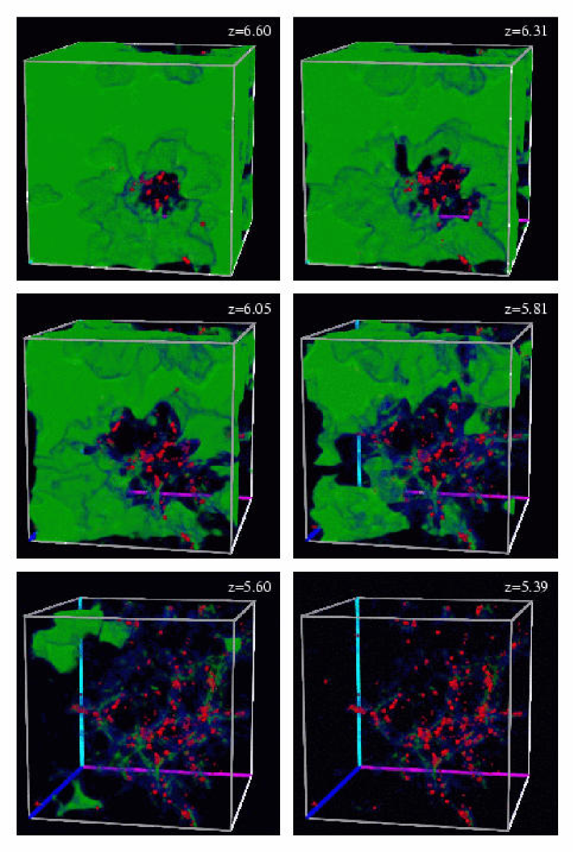
Figure 3: Volume visualization of the H i density distribution (green to blue) and star forming protogalaxies (red) at six output redshifts for the ${\epsilon_{\rm UV}}=5\times 10^{-6}$ model with stellar feedback. The first panel corresponds to the time when ionizing photons from most massive halos had already cleared their way to the nearest voids.

If two emitting cells are in immediate proximity of each other, then the cumulative effect on the IGM at some distance from these sources will be exactly equal to the sum of their individual contributions. One can treat these cells as a single point source, given that the IGM is transparent to ionizing photons within the radius of interest. Close to those sources one still might need to treat them separately, especially when the sources are just starting to ionize the surrounding medium. However, we find that once the medium close to SF regions is in a highly ionized state, we obtain virtually identical results for the ionizational state and temperature of the gas through the entire H ii region when we group neighboring point sources. A simple explanation for this result is that in either case we explicitly conserve photons and have the same balance of the number of ionizations to the number of recombinations, once the UV background establishes itself in the common H ii bubble. Stellar sources are highly clustered into few hundred halos in our $10{\rm\,Mpc}$ volume (marked by red dots in Fig. 3–5). In addition, diffuse radiation is also almost the same in both cases, since the temperature of the H ii region behind the I-front is nearly constant (Abel & Haehnelt 1999), independent of the distance to the ionizing source, while the diffuse emissivity depends mostly on the local density and not the location relative to the proto-galaxy.

To group sources together, we borrow a bottom-up tree algorithm from McMillan & Aarseth (1993). The procedure for this binning is straightforward. At each timestep, we go through all point sources in the volume and find the closest pair between which the optical depth does not exceed $\tau_{\rm min}$. If this separation is also smaller than some threshold value $d_{\rm min}$, then we merge these two sources into a new source with the location weighted by the two luminosities, and repeat the procedure of finding the closest pair with $\tau<\tau_{\rm min}$. This technique will be reasonably accurate providing that $\tau_{\rm min}$ is small enough, since in almost all cases a negligible optical depth between two sources means that each source blows a significant H ii region around them.

Note that unreasonably large values of $\tau_{\rm min}$ will bin two sources which have not had enough time to create extended H ii regions. Then, after these points are merged, the photon production site suddenly moves further from these two partially ionized regions, and now there are not enough ionizing photons to balance recombinations; as a result, the neutral fraction goes up, and at the next timestep the optical depth between the two sources jumps. Since at every timestep the tree of sources is constructed from scratch, these two sources will not be binned until they again ionize their immediate surroundings. This oscillatory behavior is a clear sign of unphysical binning and, hence, can be used as a test to choose the optimal value of $\tau_{\rm min}$. As a compromise between accuracy and speed we chose $d_{\rm min}=1.16h^{-1}{\rm\,Mpc}$ and $\tau_{\rm min}=0.1$.

3.2 Diffuse Radiation

The diffuse component coming from recombinations and bremsstrahlung in the gas and from the background UV flux are computed separately using a network of long rays crossing the entire volume. At each timestep, we calculate the emissivity of each cell and redistribute the corresponding number of photons equally among all rays crossing this cell. As we proceed along each ray, we add diffuse photons and compute sinks due to the local opacity, conserving photons explicitly.

By connecting each possible pair of boundary cells, one could ensure that every pair of cells inside the volume is connected. However, for a resolution of $N$ grid points in every direction, that would require one to compute photon conservation along $15\times N^{4}$ rays. We refer to this as the full angular resolution, and it is a prohibitively large number for $N~{}\hbox{$>$}~{}128$. Fortunately, the diffuse intensity does not exhibit as strong angular and spatial variation as direct photons from ionizing sources. Numerical tests of the sort described in Razoumov & Scott (1999) show that for the typical amount of clumping found in cosmological simulations it would suffice to use $\sim 10^{-3}$ of the number of rays one would employ with the full angular resolution, simply because radiating regions occupy a significant fraction of the volume. For example, in our $128^{3}$ simulations we get satisfactory results with $\sim 4\times 10^{6}$ rays sampling the diffuse radiation.

Emissivity from radiative recombinations and bremsstrahlung are computed using atomic models for hydrogenic and He-like ions. For hydrogenic ions the frequency-dependent recombination and free-free emissivity is (Hummer 1994)

$$\epsilon_{\nu}={{k_{\rm B}}{T_{\rm e}}\over 4\pi}{n_{\rm H}}n_{\rm ion}x_{\rm e}\left[\sum_{n=1}^{\infty}\phi_{n}({T_{\rm e}},Z,\nu)+\phi_{\rm ff}({T_{\rm e}},Z,\nu)\right],$$ (4)

where

$$\phi_{n}(T_{e},Z,\nu)={c\alpha^{3}\over\sqrt{\pi}}Z^{3}\lambda^{5/2}n^{-2}{\cal E}(1+n^{2}{\cal E})^{2}e^{-\lambda{\cal E}}\cdot{\sigma_{n}(Z,{\cal E})\over Z^{2}\nu_{1}},$$ (5)

$${\cal E}={\nu\over Z^{2}\nu_{1}},~{}~{}~{}~{}\lambda={Z^{2}h_{\rm P}\nu_{1}\over{k_{\rm B}}{T_{\rm e}}},$$ (6)

$$\phi_{\rm ff}(T_{e},Z,\nu)={8\over 3\pi^{2}}\left(\pi\over 3\right)^{1/2}\alpha^{2}\lambda_{\rm c}^{2}cZ\lambda^{1/2}e^{-u}g_{\rm ff}(u,\lambda){h_{\rm P}\over{k_{\rm B}}{T_{\rm e}}}.$$ (7)

Here $\alpha$ is the fine-structure constant, $\nu_{1}$ is the hydrogen Lyman limit, $Z$ is the atomic number, ${k_{\rm B}}$ and $h_{\rm P}$ are the Boltzmann and Planck constants, and $\sigma_{n}(Z,{\cal E})$ is the cross-section of photoionization for level $n$. Similarly, for the free-free coefficient we have introduced the free-free Gaunt factor $g_{\rm ff}(u,\lambda)$, the Compton wavelength $\lambda_{\rm c}$, and $u\equiv h\nu/{k_{\rm B}}{T_{\rm e}}$ (Hummer 1994). The quantity $n_{\rm ion}$ is either $n_{{\rm H}^{+}}$ for hydrogen or $n_{{\rm He}^{++}}$ for doubly ionized helium, while $x_{\rm e}$ is the fraction of free electrons relative to hydrogen. We take the numerical values for the hydrogenic photoionization cross-sections $\sigma_{n}(Z,{\cal E})$ from Storey & Hummer (1991) and the free-free Gaunt factor $g_{\rm ff}(u,\lambda)$ from Hummer (1988), and integrate eq. (4) numerically to get

$$\epsilon=\int_{\nu_{\rm Ly}}^{\infty}\epsilon_{\nu}d\nu$$

for our single frequency group. The expression for emissivities due to recombinations to the $nlS$ state of neutral helium is similar and can be found in Hummer & Storey (1998). In our calculations we neglect the emissivity from di-electronic recombinations of helium.

Note that the temperature of the photoionized gas does not rise above a few $\times 10^{4}$K (Abel & Haehnelt 1999). Hence, recombination and bremsstrahlung photons alone will contribute little to the radiation field above the Lyman limit and, therefore, have relatively low effect on the shape and the propagation speed of I-fronts. Of course, this does not apply to the UV background itself, which has a profound effect after the overlap of individual H ii regions.

3.3 Boundary Conditions

Direct unabsorbed photons from stellar sources inside the box are traced for two full lengths of the computational volume without the cosmological terms, assuming simple periodic boundary conditions. Once these photons reach the boundary after two lengths, they are added to the global pool of background photons. On the other hand, all diffuse (recombination, bremsstrahlung and background) photons which are already present in the volume are followed just for one full length of the box, and after crossing the boundary they are added to the pool of background photons. Thus at every timestep photons which have just been added to the background come from two contributions. We then apply the cosmological effects – dilution of radiation due to cosmic expansion and the Doppler shift – to all background photons, and using the diffuse solver we inject these photons uniformly into the photoionized part of the IGM which is already exposed to the average UV background. By construction, these are the cells for which the optical depth from the boundary (averaged over all directions) is less than unity.

3.4 Chemistry

Parallel to our RT calculation, we compute the non-equilibrium chemistry of nine species: ${\rm H}$, ${\rm H}^{+}$, ${\rm He}$, ${\rm He}^{+}$, ${\rm He}^{++}$, ${\rm H}^{-}$, ${\rm H}_{2}^{+}$, ${\rm H}_{2}$, and ${\rm e}^{-}$ (Abel et al. 1997) using the numerical algorithm described in Anninos et al. (1997). As we do raytracing for both the direct and the diffuse components, at each grid cell we store all photo-chemical reaction rates, which are then used to update ionization fractions. Similar to Sokasian et al. (2001), for recombination rates we use the clumping factor extracted from the input simulations sampled at $512^{3}$ resolution (i.e., to two levels of refinement in the AMR grid hierarchy), however, unlike in their paper, we do not assume photoionization equilibrium solving the full rate equations instead. The temperature of the medium is computed explicitly at each grid cell from energy conservation taking into account heating due to photoionizations and cooling due to radiative recombinations and bremsstrahlung, collisional excitations and collisional ionizations, molecular hydrogen cooling, as well as Compton cooling. In practice, since we do not solve hydrodynamical and radiative transfer equations simultaneously, the evolution of species other than neutral and ionized hydrogen – such as molecular hydrogen, for example – is not crucial in this model, although these species were formally included in our calculations.

3.5 Summary of Approximations

Let us briefly summarize the approximations we take. First of all, hydro and RT are computed separately, i.e. photoheating due to diffuse radiation has no dynamical effect on the gas. Secondly, we omit the time derivative in the RT equation in favor of simple photon statistics, so that at this stage we cannot properly compute ${\cal O}(v/c)$ effects. We also employ finite angular resolution for the diffuse flux, but fortunately, due to the almost isotropic nature of this diffuse component and its small value, this approximation has negligible effect on the shape and speed of I-fronts. In addition, we group nearby stellar sources once they create significant H ii regions around them. Finally, we use just one spectral group for the radiation, therefore, we cannot study He reionization in these particular calculations.

4 Results

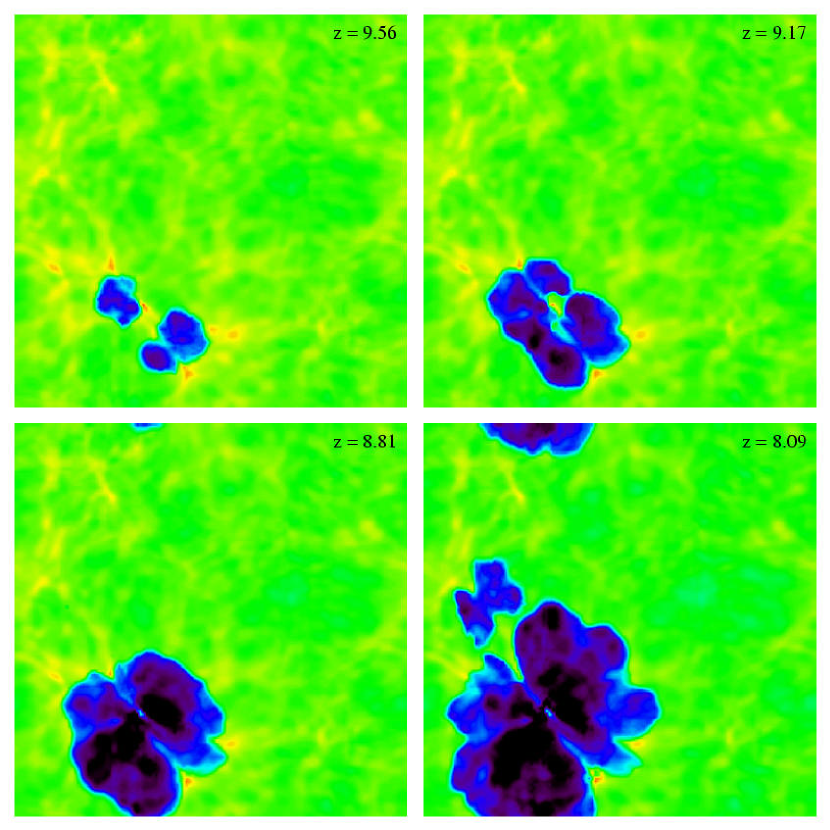
Figure 2: H i density distribution in a thin slice at four output redshifts for the ${\epsilon_{\rm UV}}=5\times 10^{-6}$ model with stellar feedback, showing how ionizing radiation breaks out into the voids.

One question which can be immediately addressed by our simulations is whether underdense regions (like voids) are ionized before overdense regions (like filaments). Our full RT simulations in a $7h^{-1}{\rm\,Mpc}$ volume show a picture of stellar reionization in which photons initially do not travel far from ionizing sources, in contrast with images from the simulations by Gnedin (2000). Fig. 2 shows that although ionizing photons stream preferentially into the voids, H ii regions do not grow bigger than a few hundred thousand kpc until after most of the gas close to sources is already ionized. This result differs from that of Gnedin (2000), who found voids ionizing before H ii regions had percolated. This counter-intuitive result stems from Gnedin’s inclusion of a homogeneous UV background which is not present in our simulation until the volume is fully ionized. In a sense, radiative transfer in our work is much more local, since the mean free path of ionizing photons in the fully ionized medium is much smaller than the box size. Host halos – and on larger scales dense filamentary structures around star forming proto-galaxies – serve as efficient sinks of radiation delaying global reionization by a significant fraction of the Hubble time. Only after these regions are ionized does radiation break out into the low-density IGM, sweeping quickly through the rest of the volume.

A related question – on how many photons per hydrogen atom would be needed to cause complete overlap – has attracted a lot of attention in recent literature (Miralda-Escudé, Haehnelt, & Rees 2000, Gnedin 2000, Haiman, Abel, & Madau 2001). In our simulations we see that about one ionizing photon per hydrogen atom in the volume has been produced by the time of overlap. However, as discussed in Gnedin (2000), such a low value is the direct result of our low resolution ($55h^{-1}{\rm\,kpc}$ comoving, or $14h^{-1}{\rm\,kpc}$ for recombinations with the $512^{3}$ clumping factor), and does not contradict the conclusion of Haiman et al. (2001) that recombinations in mini-halos (with radii of $1{\rm\,kpc}$ and smaller) would raise the required number of ionizing photons by an order of magnitude. Also note, that the assumed efficiency parameter ${\epsilon_{\rm UV}}$ already contains ${f_{\rm esc}}\sim 10\%$ if we assume the Salpeter IMF, that is, a significant fraction of ionizing photons never gets out of a resolution element. In the near future we are planning to increase our resolution to explicitly compute a larger part of the escape fraction.

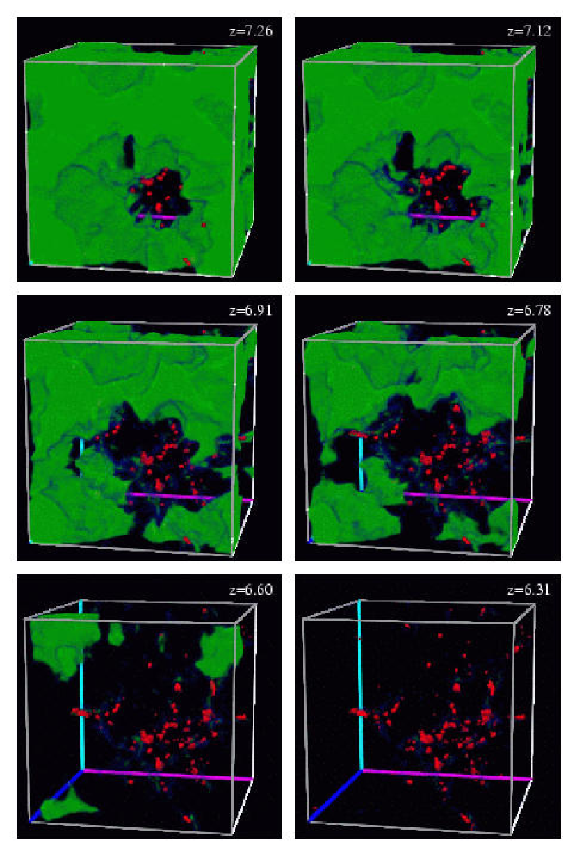
Figure 5: Same as Fig. 3 but for the ${\epsilon_{\rm UV}}=10^{-5}$ model with stellar feedback.

The two phases – initial escape and ionization of voids – are clearly separated in redshift (Fig. 2 and Fig. 3, respectively, both showing the same model). These are the ‘pre-overlap’ and the ‘overlap’ in Gnedin’s terminology, and despite the differences in the details of how photons are being deposited into the IGM in his and our models, we observe similar stages of cosmic reionization. Figs. 3 and 5 show simultaneously the 3D neutral hydrogen density distribution (green to blue in order of decreasing column density) and the location of star forming protogalaxies (red) at six output redshifts for two different UV production rates. These plots confirm that the overlap is indeed fast compared to the initial escape stage. In general, we find that the UV production efficiency in the range ${\epsilon_{\rm UV}}=5\times 10^{-6}-4\times 10^{-5}$ leads to complete overlap of H ii regions in the redshift interval $z=5.8-7.2$ (Fig. 1). Lower values of ${\epsilon_{\rm UV}}$ would not give full reionization until redshifts below those of the highest $z$ objects already known, whereas a higher luminosity output would produce too strong a UV background. The temperature of the ionized part of the IGM stays virtually constant at an average of $T\sim 16,000{\rm K}$ in the voids (see the volume-weighted temperature in the last panel in Fig. 1), rising to $20,000-40,000{\rm K}$ inside fully ionized halos, and remaining below $8,000{\rm K}$ in the neutral patches.

In Fig. 4 we plot the Gunn-Peterson optical depth (Fan et al. 2001)

$$\tau_{\rm GP}(z)=1.5\times 10^{4}h^{-1}\Omega_{\rm m}^{-1/2}\left(\Omega_{\rm b}h^{2}\over 0.02\right)\int_{0}^{z}\left(1+z^{\prime}\right)^{1/2}x_{\rm HI}(z^{\prime})dz^{\prime}$$ (8)

as a function of redshift, for two values of ${\epsilon_{\rm UV}}$ along three random lines of sight. For the assumed star formation history, the range ${\epsilon_{\rm UV}}=7$–$8\times 10^{-6}$ describes the observed statistics of very high-$z$ Ly$\alpha$ absorbers (Becker et al. 2001). The late stages of overlap already cause complete blanketing of the transmitted flux blue-ward of the redshifted Ly$\alpha$ wavelength. However, this transition in the optical depth from $\tau_{\rm GP}\sim 10^{3}$ to $\tau_{\rm GP}\sim{\rm few}$ demonstrates a scatter of $\Delta z\sim 0.2$, between different lines of sight.

After complete overlap and the rise of the UV background, the latter comes to an equilibrium with the remaining neutral patches. All of the low density gas, as well as dense filamentary regions in the vicinity of star forming protogalaxies, become fully ionized. However, a lot of the filamentary structures remain largely neutral in lower redshifts panels of Fig. 3. This is the slow ‘post-overlap’ stage observed by Gnedin (2000). The volume-weighted H i filling fraction stops falling rapidly once it reaches a plateau at $10^{-5}$–$10^{-6}$, shortly after complete overlap, with the exact number depending on the model. Ly$\alpha$ clouds are still being ionized at lower redshifts, although in two of our models with ongoing gravitational collapse recombinations are starting to dominate overall in the volume around $z=4$. Note, however, that the final neutral hydrogen fraction, as well as the UV background value would also be sensitive to the size of the box. This is because our volume is not sufficiently large to have proper statistics of damped Lyman limit systems, and, as a result, we somewhat overestimate the value of the background field.

5 Discussion

Our current simulations demonstrate the feasibility of a full radiative transfer calculation, in which a constantly evolving density field and a source function could be computed self-consistently within a hydro code. In a forthcoming paper, we will couple our radiative transfer method with the enzo (Bryan & Norman 1999) hydro code. The algorithm developed in this paper extends the achievable resolution limit by combining both ray segments and sources into hierarchical tree structures as we move farther from host proto-galaxies. A further step would be to make the scheme adaptive on many levels. Developing fully adaptive mesh refinement RT simulations is a long-term goal. In the meantime one could devise an array of shortcuts in order to speed up RT calculations. For example, ray trees can be build in such a way that they accurately capture narrow I-fronts without the need for performing excessive calculations in the rest of the volume. One possible solution is to keep photo-chemical reaction rates constant, without computing full RT in already ionized or yet fully neutral regions, updating these rates only every 10th or 100th timestep (Sokasian et al., 2001). Many such measures will be tried as we make collective progress towards modeling the physics of radiation as realistically as possible in cosmological simulations. We believe that our current computations represent a significant step along this path.

The goal of this paper has been to present self-consistent inhomogeneous radiative transfer in a fairly large cosmological volume filled with young star-forming galaxies and ‘dark’ extended absorbers. At this point we cannot directly compute the physical escape fraction of ionizing photons from their host halos, both due to poorly constrained physics at sub-galactic scales and also due to the present lack of spatial resolution. Instead we have to rely on parameterizing the escape fraction within an effective UV efficiency factor. However, the technique described here – when combined with the power of AMR within hydro simulations – can bring us closer to a correct quantitative description of the relevant galaxy formation processes, both prior to and after the beginning of cosmic reionization. Ideally, these models should be combined with the full frequency-dependent physics of a code such as CUBA (Haardt & Madau 2001) to perform exact matching between numerical star formation and the observed quantities at lower redshifts, such as the UV background or directly measured luminosity functions.

Recently obtained spectra of the highest redshift quasars (Becker et al. 2001, Djorgovski et al. 2001) show tantalizing evidence for the end of the reionization process occurring at $z\simeq 6$. It may therefore be possible to obtain data in the near future which directly probes the reionization process. The redshift evolution and spatial topology of reionization may be measurable using sufficiently many lines of sight. Comparison with models such as ours may allow connections to be made between the observational diagnostics and physical inputs to the reionization process: IMFs, SF rates, relative contributions of AGN, sizes of the first collapsing mini-halos, etc. A suite of simulations along the lines of those described here will be extremely helpful in fulfilling this goal.

Figure 1: Upper left panel: redshift-normalized average star formation rate (in ${\rm\,M_{\odot}}{\rm\,Mpc}^{-3}$ per unit redshift interval), with (solid line) and without (dashed line) stellar feedback. Lower left panel: spatially-averaged Lyman-limit background intensity (in ${\rm\,erg}{\rm\,cm}^{-2}{\rm\,s}^{-1}{\rm\,Hz}^{-1}{\rm\,sr}^{-1}$) as a function of redshift for models with ${\epsilon_{\rm UV}}=5\times 10^{-6}$ (short-dashed line), $8\times 10^{-6}$ (long-dashed line), $10^{-5}$ (solid line), and $4\times 10^{-5}$ (dash-double-dotted line) with stellar feedback, and the dash-dotted line shows the model with ${\epsilon_{\rm UV}}=5\times 10^{-6}$ and no stellar feedback. The three dotted lines show the integrated UV background if there were no absorbing medium in the volume, for the same amount of star formation at ${\epsilon_{\rm UV}}=10^{-5}$, $8\times 10^{-6}$ and $5\times 10^{-6}$ from top to bottom, respectively. Upper right panel: volume-weighted (four thin lines) and mass-weighted (two thick lines) H i filling fraction, for models with stellar feedback and ${\epsilon_{\rm UV}}=10^{-5}$ (solid line), $8\times 10^{-6}$ (long-dashed line), $5\times 10^{-6}$ (short-dashed line), and without stellar feedback and ${\epsilon_{\rm UV}}=5\times 10^{-6}$ (dash-dotted line). Lower right panel: total (solid line), H i (short-dashed line) and H ii (dotted line) clumping factors, and volume-weighted temperature (thick long-dashed line), for ${\epsilon_{\rm UV}}=5\times 10^{-6}$ with stellar feedback.

Figure 4: Gunn-Peterson optical depth for models with stellar feedback and ${\epsilon_{\rm UV}}=5\times 10^{-6}$ (solid lines) and ${\epsilon_{\rm UV}}=8\times 10^{-6}$ (dotted lines), along three random lines of sight.

References

- Abel et al. (1997) Abel, T., Anninos, P., Zhang, Y., & Norman, M. L. 1997, New Astronomy, 2, 181
- Abel (2000) Abel, T. 2000, Revista Mexicana de Astronomia y Astrofisica Conference Series, 9, 300
- Abel & Haehnelt (1999) Abel, T., & Haehnelt, M. G. 1999, ApJ, 520, L13
- Abel et al. (1999) Abel, T., Norman, M. L., & Madau, P. 1999, ApJ, 523, 66
- Abel & Wandelt (2001) Abel, T., & Wandelt, B. D. 2001, astro-ph/0111033
- Anninos et al. (1997) Anninos, P., Zhang, Y., Abel, T., & Norman, M. L. 1997, New Astronomy, 2, 209
- Becker et al. (2001) Becker, R. H., et al. 2001, AJ, in press, astro-ph/0108097
- Bryan & Norman (1999) Bryan G. L., & Norman M. L. 1999, in IMA Vol. 117, Structured Adaptive Mesh Refinement (SAMR) Grid Methods, ed. S. B. Baden, N. P. Chrisochoides, D. Gannon, & M. L. Norman (New York: Springer), 165
- Cen & Ostriker (1993) Cen, R., & Ostriker, J. P. 1993, ApJ, 417, 404
- Chiu & Ostriker (2000) Chiu, W. A., & Ostriker, J. P. 2000, ApJ, 534, 507
- Ciardi et al. (2000) Ciardi, B., Ferrara, A., Governato, F., & Jenkins, A. 2000, MNRAS, 314, 611
- Ciardi et al. (2001) Ciardi, B., Ferrara, A., Marri, S., & Raimondo, G. 2001, MNRAS, 324, 381
- Djorgovski et al. (2001) Djorgovski, S. G., Castro, S. M., Stern, D., Mahaba, A. 2001, ApJ, in press, astro-ph/0108069
- Fan et al. (2001) Fan, X. et al. 2001, AJ, submitted, astro-ph/0108063
- Gnedin (2000) Gnedin, N. Y. 2000, ApJ, 535, 530
- Gnedin & Abel (2001) Gnedin, N. Y., & Abel, T. 2001, astro-ph/0106278
- Gnedin & Ostriker (1997) Gnedin, N. Y., & Ostriker, J. P. 1997, ApJ, 486, 581
- Haardt & Madau (1996) Haardt, F., & Madau, P. 1996, ApJ, 461, 20
- Haardt & Madau (2001) Haardt, F., & Madau, P. 2001, astro-ph/0106018
- Haiman et al. (2001) Haiman, Z., Abel, T., & Madau, P. 2001, ApJ, 551, 599
- Hummer (1988) Hummer, D. G. 1988, ApJ, 327, 477
- Hummer (1994) Hummer, D. G. 1994, MNRAS, 268, 109
- Hummer & Storey (1998) Hummer, D. G., & Storey, P. J. 1998, MNRAS, 297, 1073
- Loeb & Barkana (2001) Loeb, A., & Barkana, R. 2001, ARA&A, 39, 19
- McMillan & Aarseth (1993) McMillan, S. L. W., & Aarseth, S. J. 1993, ApJ, 414, 200
- Miralda-Escudé, Haehnelt, & Rees (2000) Miralda-Escudé, J., Haehnelt, M., & Rees, M. J. 2000, ApJ, 530, 1
- Norman et al. (1998) Norman, M. L., Paschos, P., & Abel, T. 1998, Memorie della Soc. Astron. Italiana, 69, 455
- Razoumov & Scott (1999) Razoumov, A. O., & Scott, D. 1999, MNRAS, 309, 287
- Seljak & Zaldarriaga (1996) Seljak, U., Zaldarriaga, M. 1996, ApJ, 469, 437
- Sokasian et al. (2001) Sokasian, A., Abel, T., & Hernquist, L. E. 2001, astro-ph/0105181
- Storey & Hummer (1991) Storey, P. J., & Hummer, D. G. 1991, Comput. Phys. Commun., 66, 129
- Umemura, Nakamoto & Susa (1998) Umemura, M., Nakamoto, T., & Susa, H. 1998, in Numerical Astrophysics 1998, ed. S. M. Miyama & K. Shibata (Kluwer)
- Valageas & Silk (1999) Valageas, P., & Silk, J. 1999, A&A, 347, 1