Multiplicity of X-Ray Selected T Tauri Stars in Chamaeleon

Abstract

We report on a multiplicity survey of a sample of X-ray selected young stars in the Chamaeleon association. We used speckle-interferometry and direct imaging to find companions in the separation range $0.13^{\prime\prime}$ to $6^{\prime\prime}$. After correction for chance alignment with background stars, we find a multiplicity (number of binaries or multiples divided by number of systems) of $(14.0\pm 4.3)\,\%$ and a companion star frequency (number of companions divided by number of systems) of $(14.7\pm 5.1)\,\%$. Compared to solar-type main-sequence stars, the companion star frequency is lower by a factor of $0.61\pm 0.27$. This is remarkably different from the high multiplicity found in the Taurus-Auriga star-forming region and for T Tauri stars in Chamaeleon known before ROSAT. We find only a few binaries with projected separations of more than 70 AU, also in contrast to the results for stars known before ROSAT. This indicates that the X-ray selected stars belong to a different population than the stars known before ROSAT, a hypothesis further supported by their Hipparcos distances and proper motions.

1 Introduction

Recent studies of multiplicity in several star-forming regions have shown that multiplicity is – besides the initial mass function – one of the key characteristics of the star-formation process. Surveys of T Tauri stars (TTS) in the T association Taurus-Auriga (Leinert et al., 1993; Ghez et al., 1993; Köhler & Leinert, 1998) found an overabundance of binaries compared to solar-type main-sequence stars (Duquennoy & Mayor, 1991) by a factor of two. On the other hand, surveys of low-mass stars in the Orion Trapezium Cluster (Prosser et al., 1994; Padgett et al., 1997; Petr et al., 1998) found a multiplicity that is comparable to or even lower than among main-sequence stars. Scally et al. (1999) used proper motion data of stars in the Trapezium cluster to search for binaries with separations in the range 1000 to 5000 AU. Their statistical analysis shows that the cluster contains no binaries at all in this separation range. Studies of other clusters (Duchêne et al., 1999, IC348:; Bouvier et al., 1997, Pleiades:) also found a binary frequency comparable to main-sequence stars. An explanation for these results is the disruption of binaries in stellar encounters, which happen predominantly in dense clusters (Kroupa, 1995b). However, it is also possible that the multiplicity depends on environmental parameters like magnetic fields or the cloud temperature (e.g. Durisen & Sterzik, 1994).

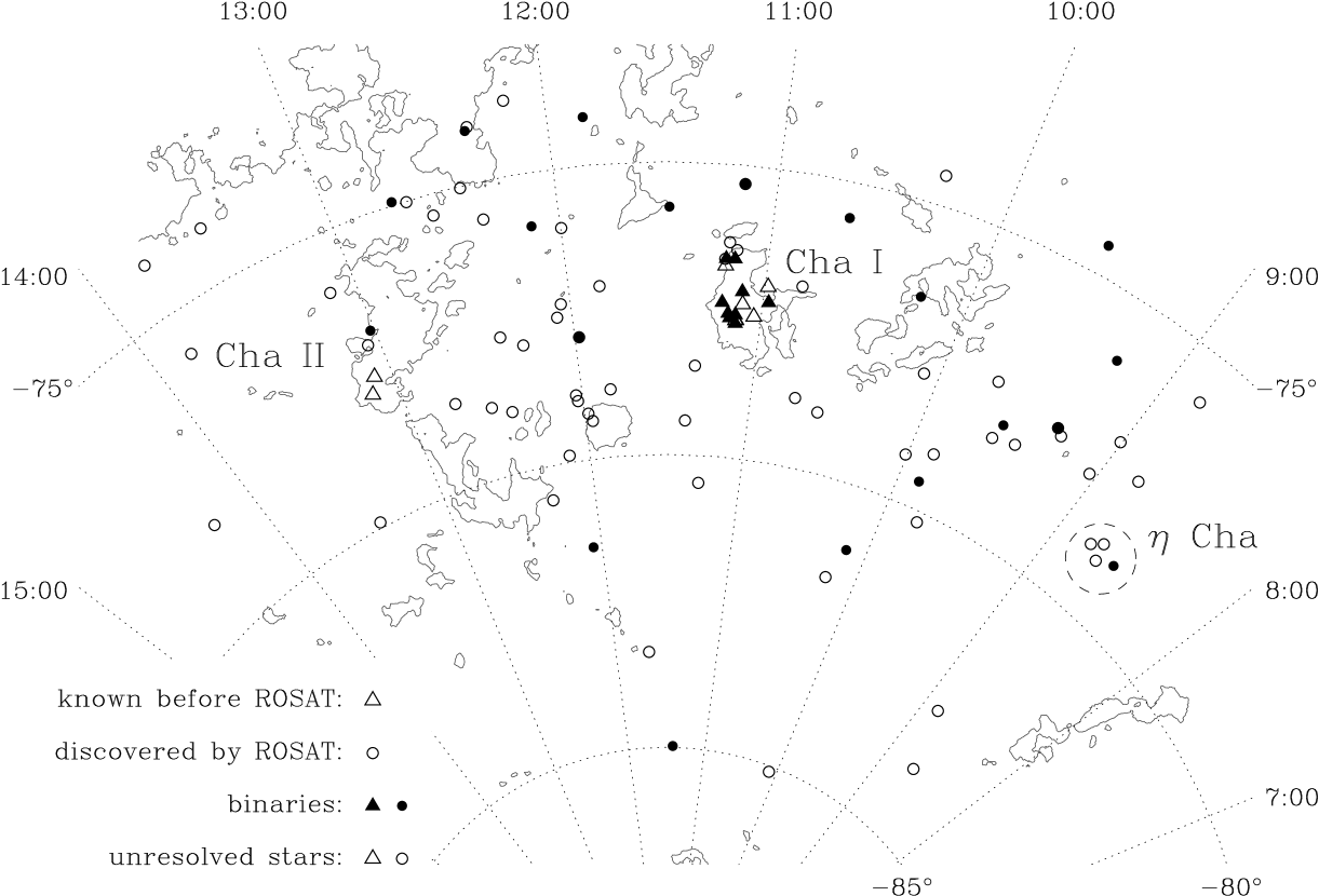
Figure 1: Spatial distribution of the stars in our sample and the sample of Ghez et al. (1997). The contours mark the emission found in the IRAS $100\rm\,\mu m$ survey. Cha I and II are the cloud complexes where most TTS known before ROSAT are located. The large dashed circle encloses the four stars in the $\eta$ Chamaeleontis cluster (Mamajek et al., 1999).

Kroupa (1995a) proposed to use the binary frequency and their distribution of periods to determine the dominant mode of star formation, i.e. if most stars form in dense regions like the Orion Cluster, or in loose associations like Taurus-Auriga (“inverse population synthesis”). However, although Taurus-Auriga is the best studied T association, it is by no means clear that it is a typical example with respect to the formation of binaries. Some authors surveyed other star-forming regions (Reipurth & Zinnecker, 1993; Brandner et al., 1996; Ghez et al., 1997), but the number of stars observed or the spatial resolution was very limited, which causes large statistical errors. Furthermore, it turned out that even within one star-forming region (Scorpius-Centaurus), the period distribution of binaries in two subregions can be significantly different (Brandner & Köhler, 1998; Köhler et al., 2000). We can expect to find even larger differences between different star-forming regions.

In the light of these results, it is desirable to conduct a survey of a large number of stars in other T associations, in order to find out if Taurus-Auriga is a typical example or the exception to the rule. Thanks to the ROSAT All-Sky Survey, sufficiently large samples of TTS are available for the T associations Chamaeleon and Lupus. We carried out multiplicity surveys for both of them. This paper describes the survey in Chamaeleon, Lupus will be presented elsewhere.

Ghez et al. (1997) already searched for binaries among TTS in Chamaeleon. However, only the observations of 17 stars were sensitive enough to give meaningful results. Furthermore, they observed only stars known before ROSAT, i.e. stars located on or near the dark clouds and mainly Classical T Tauri stars (CTTS). The results of the ROSAT All-Sky survey have shown that pre-main-sequence stars can be found in much larger areas around star-forming regions, and that the majority of pre-main-sequence stars are Weak-line T Tauri stars (WTTS; Walter et al. 1988; Neuhäuser et al. 1995).

Our survey encompasses a list of WTTS found with the help of ROSAT. Section 2 describes the object list and section 3 our observations and data reduction. The results are presented and discussed in section 3 and 4, while section 5 contains the summary and conclusions.

2 The Sample

Our survey is based on the results of Alcalá et al. (1995) and Covino et al. (1997). Alcalá et al. did follow-up observations of optical counterparts of X-ray sources in the Chamaeleon region detected in the ROSAT All-Sky Survey. They identified 82 young low-mass stars based on the presence of the Li $\lambda 6707$ absorption line and the spectral type. A complete list with coordinates, photometric data, and finding charts can be found in Alcalá et al. (1995). Fig. 1 shows the spatial distribution of these stars and the stars observed by Ghez et al. (1997).

The four stars around $\rm 8^{h}42^{m}$, $-79^{\circ}$ are probably members of the $\eta$ Chamaeleontis cluster (Mamajek et al., 1999). Our results for these stars are listed in Table 1 and 2, but we do not use them for the discussion of the binary properties in the Chamaeleon star-forming region. The binaries in $\eta$ Cha will be discussed in Köhler (2001). Two sources (RXJ 1039.5-7538 (catalog )N+S) are separated by only $5^{\prime\prime}$, therefore we count them as one binary. This leaves us with a sample of $82-4-1=77$ systems.

It has been questioned recently (Briceño et al., 1997) whether stars found with low-resolution spectroscopy are indeed pre-main-sequence (PMS) objects or if they are somewhat older stars which have already reached the zero-age main-sequence (ZAMS). In order to unambiguously distinguish PMS and ZAMS objects, Covino et al. (1997) carried out observations with high spectral resolution of some 70 stars of the sample. They compared the equivalent width of the Li $\lambda 6707$ line to that of Pleiades stars of the same spectral type and classified the stars as PMS or ZAMS. They found that more than 50 % of the stars could be confirmed to be PMS objects.

3 Observations and Data Reduction

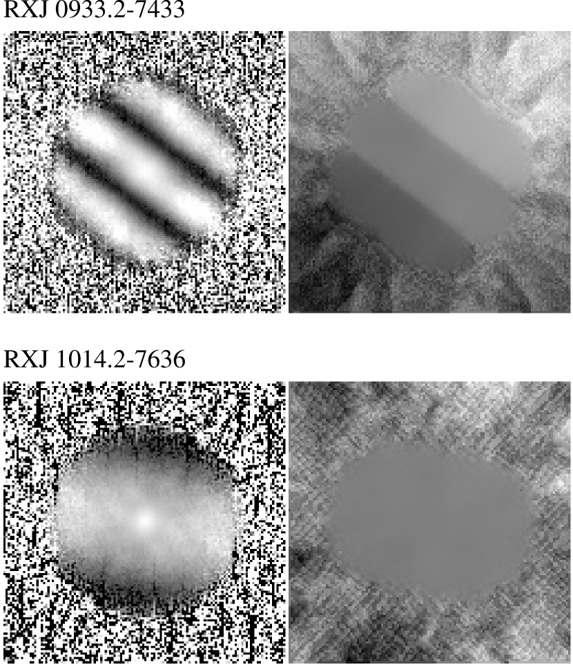
Figure 2: Examples of our speckle data. The images in the first row show modulus (left) and phase (right) of the complex visibility of RXJ 0933.2-7433, a close, but well-resolved binary. The central maximum and the first maximum on both sides are clearly detected. The second row shows modulus and phase of RXJ 1014.2-7636, a potential binary closer than the diffraction limit of the telescope. In this case, we see only the central maximum and the first minimum on each side.

The speckle observations were carried out at the ESO 3.5 m New Technology Telescope (NTT) on La Silla, Chile, from 29. March to 2. April 1996. We used the SHARP I camera (System for High Angular Resolution Pictures) of the Max-Planck-Institut for Extraterrestrial Physics (Hofmann et al., 1992). All observations were done in the K-band at $2.2\rm\,\mu m$.

Although speckle interferometry can be considered by now a standard technique (Leinert, 1992), no program for speckle data reduction was publicly available at the time this survey was started. Therefore we used our speckle program, which was already used for the surveys in Taurus-Auriga (Köhler & Leinert, 1998) and Scorpius-Centaurus (Köhler et al., 2000). In this program, the modulus of the complex visibility (i.e. the Fourier transform of the object brightness distribution) is determined from power spectrum analysis, the phase is computed using the Knox-Thompson algorithm (Knox & Thompson, 1974), and from the bispectrum (Lohmann et al., 1983). Figure 2 shows examples of reconstructed complex visibilities. For a more detailed description see Köhler et al. (2000).

Figure 3: The results of our multiplicity survey in a plot of flux ratio or magnitude difference vs. binary star separation. The data points mark the detected companion stars, the thick line shows the average and the thin line the worst sensitivity for undetected companions. The dashed vertical line at $0.13^{\prime\prime}$ shows the diffraction limit for a $3.5\rm\,m$ telescope at K. This is the limit for unambiguous identification of binary stars. The dashed horizontal line shows the completeness limit in flux ratio for the whole survey. The two observations of RXJ 1039.5-7538 are represented by two data points connected by a line.

If the object appears unresolved, we compute the maximum brightness ratio of a companion that could be hidden in the noise of the data. The principle is to determine how far the data deviate from the nominal result for a point source (modulus${}=1$, phase${}=0$). We then compute the maximum brightness ratio of a companion that would be compatible with this amount of deviation. This is repeated for different position angles, and the maximum is used as upper limit for the brightness ratio of an undetected companion. See Leinert et al. (1997) for a more detailed description of this procedure.

If the object is a binary or triple, we compute a multidimensional least-squares fit using the amoeba algorithm (Press et al., 1994). Our program tries to minimize the difference between modulus and phase computed from a model binary or triple and the observational data by varying the separation, position angle, and brightness ratio of the model. This is necessary because the reconstructed images are a complex function of the 2-dimensional separation vector and flux ratio that cannot be solved to compute the binary parameters directly from the data. Fits to different subsets of the data yield an estimate for the standard deviation of the binary parameters. We then subtract the contribution of the companion(s) from the images and apply the procedure described in the previous paragraph to find limits for the brightness of an undetected companion.

In order to find binaries that are separated by more than $3^{\prime\prime}$, we obtained additional infrared images with the ESO/MPIA $2.2\rm\,m$ telescope on La Silla in February and March 1996 using the IRAC2b camera. For data reduction, we used the Daophot package within IRAF.

4 Results

4.1 Uncorrected Data

All the binary and multiple stars we find in our sample are listed in Table 1, while Table 2 gives limits for the brightness of undetected companions. Figure 3 shows these results as a plot of flux ratio and magnitude difference vs. binary separation. In total, among the 81 systems of the sample we find 18 binaries and one triple star.

The modulus of the complex visibility of a binary is a cosine-shaped function. If the separation of the binary is equal to the diffraction limit ($0.13^{\prime\prime}$ for a $3.5\rm\,m$ telescope at K), exactly one period of the modulus of the visibility fits within the radius where the optical transfer function of the telescope is not zero. Under good circumstances, it is possible to discover binaries with even smaller separations, down to about half the diffraction limit (Table 1 shows that we actually do find some, an example is presented in Figure 2). However, in these cases we can detect only the first minimum, but not the second maximum of the modulus of the visibility. Therefore, we cannot distinguish with certainty a close binary star from an elongated structure. Even more important, we cannot be sure that we find all companions at separations less than the diffraction limit. For these reasons, we limit ourselves to companions in the separation range between $0.13^{\prime\prime}$ and $6^{\prime\prime}$. The upper limit was chosen so that contamination with background stars has little effect (see section 4.3 for a detailed discussion of this problem).

We found four binaries with separations smaller than $0.13^{\prime\prime}$. These binaries are treated as unresolved stars in our survey. This leaves 14 binaries and one triple, i. e. 16 companion stars, including one binary in the $\eta$ Cha cluster. For ease of comparison we mention that these uncorrected data correspond to a fractional multiplicity (number of multiples divided by total number of systems) of $0.19\pm 0.05$ or to a number of $0.20\pm 0.05$ companions per primary. These numbers change to $0.18\pm 0.05$ and $0.19\pm 0.05$ if we exclude the four stars in the $\eta$ Chamaeleontis cluster.

4.2 Completeness

Figure 3 shows not only the stars where we find companions, but also the sensitivity of our survey, i. e. the maximum brightness ratio of a possible undetected companion as a function of the separation. This sensitivity depends on factors like the atmospheric conditions at the time of the observations and the brightness of the target star. Fig. 3 and Table 2 show that in most cases we are able to detect companions with magnitude differences to the primary up to (at least) $2.5^{\rm mag}$. This corresponds to a brightness ratio of 1:10.

Our observations of four stars are not sufficiently sensitive to exclude faint companions at small separations. However, based on the number of companions actually found, we expect about 0.3 additional companions above a brightness ratio of 1:10 at separations ${}>0.13^{\prime\prime}$. Therefore, we are confident we have found all companions with separations between $0.13^{\prime\prime}$ and $6^{\prime\prime}$ and with a magnitude difference of less than $2.5^{\rm mag}$.

Table 1: Binary and triple stars.

No.	Designation		Evol.	Date of	Separation		Position		Brightness
			Status	Observation	[$"$]		Angle [∘]		Ratio at K
1	RXJ 0837.0-7856		PMS	29. Mar. 96	0.135${}\pm$	0.003	15.9${}\pm$	1.8	0.805 ${}\pm$	0.024
11	RXJ 0915.5-7609		PMS	30. Mar. 96	0.111${}\pm$	0.007	292.5${}\pm$	4.3	0.255 ${}\pm$	0.02
13	RXJ 0919.4-7738N		?	30. Mar. 96	0.109${}\pm$	0.003	173.9${}\pm$	1.2	0.658 ${}\pm$	0.021
16	RXJ 0933.2-7433		ZAMS	31. Mar. 96	0.222${}\pm$	0.003	231.4${}\pm$	0.4	0.743 ${}\pm$	0.034
17	RXJ 0935.0-7804		PMS	31. Mar. 96	0.360${}\pm$	0.003	353.9${}\pm$	0.2	0.901 ${}\pm$	0.022
22	RXJ 0952.7-7933		?	31. Mar. 96	0.267${}\pm$	0.003	314.6${}\pm$	0.5	0.259 ${}\pm$	0.018
26	RXJ 1009.6-8105		?	28. Feb. 96	5.413${}\pm$	0.017	136.9${}\pm$	0.3	0.039 ${}\pm$	0.001
27	RXJ 1014.2-7636		?	1. Apr. 96	0.091${}\pm$	0.007	259.6${}\pm$	6.5	0.593 ${}\pm$	0.062
31/32	RXJ 1039.5-7538N+S		?	26. Feb. 96	4.962${}\pm$	0.022	347.4${}\pm$	0.2	0.287 ${}\pm$	0.003
				30. Mar. 96	5.002${}\pm$	0.003	347.5${}\pm$	0.1	0.264 ${}\pm$	0.004
36	RXJ 1108.8-7519b		PMS	30. Mar. 96	0.150${}\pm$	0.003	7.8${}\pm$	1.7	0.716 ${}\pm$	0.019
43	RXJ 1125.8-8456		?	26. Feb. 96	3.545${}\pm$	0.022	208.0${}\pm$	0.2	0.140 ${}\pm$	0.003
44	RXJ 1129.2-7546		PMS	29. Mar. 96	0.534${}\pm$	0.003	28.7${}\pm$	0.2	0.189 ${}\pm$	0.008
48	RXJ 1150.9-7411		?	1. Apr. 96	0.875${}\pm$	0.003	106.0${}\pm$	0.1	0.257 ${}\pm$	0.012
50	RXJ 1158.5-7754a		PMS	29. Mar. 96	0.073${}\pm$	0.006	160.8${}\pm$	2.8	0.506 ${}\pm$	0.089
57	RXJ 1203.7-8129		?	31. Mar. 96	0.396${}\pm$	0.003	238.3${}\pm$	0.1	0.775 ${}\pm$	0.008
60	RXJ 1207.9-7555		?	1. Apr. 96	0.588${}\pm$	0.003	10.2${}\pm$	0.2	0.924 ${}\pm$	0.02
65	RXJ 1220.4-7407		PMS	1. Apr. 96	0.296${}\pm$	0.003	348.4${}\pm$	1.2	0.258 ${}\pm$	0.021
73	RXJ 1243.1-7458	A-B	PMS	30. Mar. 96	0.280${}\pm$	0.004	84.7${}\pm$	3.6	0.386 ${}\pm$	0.025
		AB-C		30. Mar. 96	2.513${}\pm$	0.003	258.7${}\pm$	0.1	0.244 ${}\pm$	0.007
75	RXJ 1301.0-7654		PMS	30. Mar. 96	1.444${}\pm$	0.005	3.2${}\pm$	0.2	0.155 ${}\pm$	0.01

Table 2: Limits for the brightness of undetected companions.

No.	Designation	Evol.	Date of	Maximum Flux Ratio		Minimal $\Delta m_{\rm K}$ [mag]
		Status	Observation	at $0.13^{\prime\prime}$	at $0.5^{\prime\prime}$	at $0.13^{\prime\prime}$	at $0.5^{\prime\prime}$
1	RXJ 0837.0-7856 (catalog )	PMS	29. Mar. 96	0.04	0.01	3.49	5.00
2	RXJ 0842.4-8345 (catalog )	?	30. Mar. 96	0.05	0.02	3.25	4.25
3	RXJ 0842.9-7904 (catalog )	PMS	29. Mar. 96	0.05	0.01	3.25	5.00
4	RXJ 0844.5-7846 (catalog )	PMS	29. Mar. 96	0.05	0.02	3.25	4.25
5	RXJ 0848.0-7854 (catalog )	PMS	29. Mar. 96	0.05	0.02	3.25	4.25
6	RXJ 0849.2-7735 (catalog )	?	29. Mar. 96	0.04	0.01	3.49	5.00
7	RXJ 0850.1-7554 (catalog )	PMS	29. Mar. 96	0.06	0.01	3.05	5.00
8	RXJ 0853.1-8244 (catalog )	?	30. Mar. 96	0.05	0.02	3.25	4.25
9	RXJ 0901.0-7715 (catalog )	?	30. Mar. 96	0.2	0.07	1.75	2.89
10	RXJ 0902.9-7759 (catalog )	PMS	30. Mar. 96	0.05	0.02	3.25	4.25
11	RXJ 0915.5-7609 (catalog )	PMS	30. Mar. 96	0.05	0.01	3.25	5.00
12	RXJ 0917.2-7744 (catalog )	?	30. Mar. 96	0.07	0.01	2.89	5.00
13	RXJ 0919.4-7738N (catalog )	?	30. Mar. 96	0.04	0.01	3.49	5.00
14	RXJ 0919.4-7738S (catalog )	?	30. Mar. 96	0.17	0.07	1.92	2.89
15	RXJ 0928.5-7815 (catalog )	?	30. Mar. 96	0.08	0.02	2.74	4.25
16	RXJ 0933.2-7433 (catalog )	ZAMS	31. Mar. 96	0.06	0.01	3.05	5.00
17	RXJ 0935.0-7804 (catalog )	PMS	31. Mar. 96	0.04	0.01	3.49	5.00
18	RXJ 0936.3-7820 (catalog )	?	31. Mar. 96	0.06	0.02	3.05	4.25
19	RXJ 0942.7-7726 (catalog )	PMS	31. Mar. 96	0.03	0.01	3.81	5.00
20	RXJ 0946.9-8011 (catalog )	?	31. Mar. 96	0.05	0.03	3.25	3.81
21	RXJ 0951.9-7901 (catalog )	PMS	31. Mar. 96	0.04	0.02	3.49	4.25
22	RXJ 0952.7-7933 (catalog )	?	31. Mar. 96	0.05	0.01	3.25	5.00
23	RXJ 1001.1-7913 (catalog )	PMS	31. Mar. 96	0.05	0.01	3.25	5.00
24	RXJ 1005.3-7749 (catalog )	PMS	1. Apr. 96	0.06	0.01	3.05	5.00
25	RXJ 1007.7-8504 (catalog )	?	1. Apr. 96	0.05	0.01	3.25	5.00
26	RXJ 1009.6-8105 (catalog )	?	1. Apr. 96	0.06	0.02	3.05	4.25
27	RXJ 1014.2-7636 (catalog )	?	1. Apr. 96	0.05	0.01	3.25	5.00
28	RXJ 1014.4-8138 (catalog )	?	1. Apr. 96	0.04	0.02	3.49	4.25
29	RXJ 1017.9-7431 (catalog )	ZAMS	1. Apr. 96	0.05	0.02	3.25	4.25
30	RXJ 1035.8-7859 (catalog )	ZAMS	30. Mar. 96	0.06	0.03	3.05	3.81
31/32	RXJ 1039.5-7538N+S (catalog )	?	30. Mar. 96	0.12	0.05	2.30	3.25
33	RXJ 1044.6-7849 (catalog )	ZAMS	30. Mar. 96	0.10	0.02	2.50	4.25
34	RXJ 1048.9-7655 (catalog )	?	30. Mar. 96	0.06	0.03	3.05	3.81
35	RXJ 1108.8-7519a (catalog )	PMS	30. Mar. 96	0.13	0.04	2.22	3.49
36	RXJ 1108.8-7519b (catalog )	PMS	30. Mar. 96	0.05	0.01	3.25	5.00
37	RXJ 1109.4-7627 (catalog )	PMS	30. Mar. 96	0.09	0.02	2.61	4.25
38	RXJ 1111.7-7620 (catalog )	PMS	30. Mar. 96	0.06	0.03	3.05	3.81
39	RXJ 1112.7-7637 (catalog )	PMS	29. Mar. 96	0.07	0.05	2.89	3.25
40	RXJ 1117.0-8028 (catalog )	PMS	30. Mar. 96	0.05	0.03	3.25	3.81
41	RXJ 1120.3-7828 (catalog )	?	29. Mar. 96	0.04	0.02	3.49	4.25
42	RXJ 1123.2-7924 (catalog )	PMS	30. Mar. 96	0.07	0.05	2.89	3.25
43	RXJ 1125.8-8456 (catalog )	?	30. Mar. 96	0.05	0.02	3.25	4.25
44	RXJ 1129.2-7546 (catalog )	PMS	29. Mar. 96	0.05	0.01	3.25	5.00
45	RXJ 1140.3-8321 (catalog )	?	30. Mar. 96	0.03	0.03	3.81	3.81
46	RXJ 1149.8-7850 (catalog )	PMS	1. Apr. 96	0.04	0.03	3.49	3.81
47	RXJ 1150.4-7704 (catalog )	PMS	29. Mar. 96	0.10	0.02	2.50	4.25
48	RXJ 1150.9-7411 (catalog )	?	1. Apr. 96	0.08	0.01	2.74	5.00
49	RXJ 1157.2-7921 (catalog )	PMS	29. Mar. 96	0.10	0.03	2.50	3.81
50	RXJ 1158.5-7754a (catalog )	PMS	29. Mar. 96	0.03	0.01	3.81	5.00
51	RXJ 1158.5-7754b (catalog )	PMS	29. Mar. 96	0.05	0.03	3.25	3.81
52	RXJ 1158.5-7913 (catalog )	PMS	29. Mar. 96	0.06	0.01	3.05	5.00
53	RXJ 1159.7-7601 (catalog )	PMS	31. Mar. 96	0.02	0.01	4.25	5.00
54	RXJ 1201.7-7859 (catalog )	PMS	31. Mar. 96	0.06	0.01	3.05	5.00
55	RXJ 1202.1-7853 (catalog )	PMS	31. Mar. 96	0.04	0.01	3.49	5.00
56	RXJ 1202.8-7718 (catalog )	?	31. Mar. 96	0.03	0.01	3.81	5.00
57	RXJ 1203.7-8129 (catalog )	?	31. Mar. 96	0.03	0.01	3.81	5.00
58	RXJ 1204.6-7731 (catalog )	PMS	31. Mar. 96	0.04	0.01	3.49	5.00
59	RXJ 1207.7-7953 (catalog )	?	1. Apr. 96	0.07	0.03	2.89	3.81
60	RXJ 1207.9-7555 (catalog )	?	1. Apr. 96	0.04	0.01	3.49	5.00
61	RXJ 1209.8-7344 (catalog )	?	1. Apr. 96	0.04	0.02	3.49	4.25
62	RXJ 1216.8-7753 (catalog )	PMS	1. Apr. 96	0.10	0.04	2.50	3.49
63	RXJ 1217.4-8035 (catalog )	?	1. Apr. 96	0.07	0.01	2.89	5.00
64	RXJ 1219.7-7403 (catalog )	PMS	1. Apr. 96	0.04	0.02	3.49	4.25
65	RXJ 1220.4-7407 (catalog )	PMS	1. Apr. 96	0.05	0.01	3.25	5.00
66	RXJ 1220.6-7539 (catalog )	?	1. Apr. 96	0.03	0.01	3.81	5.00
67	RXJ 1223.5-7740 (catalog )	?	1. Apr. 96	0.04	0.02	3.49	4.25
68	RXJ 1224.8-7503 (catalog )	?	1. Apr. 96	0.04	0.02	3.49	4.25
69	RXJ 1225.3-7857 (catalog )	?	1. Apr. 96	0.08	0.01	2.74	5.00
70	RXJ 1231.9-7848 (catalog )	?	1. Apr. 96	0.06	0.03	3.05	3.81
71	RXJ 1233.5-7523 (catalog )	?	30. Mar. 96	0.04	0.02	3.49	4.25
72	RXJ 1239.4-7502 (catalog )	PMS	29. Mar. 96	0.05	0.01	3.25	5.00
73	RXJ 1243.1-7458 (catalog )	PMS	30. Mar. 96	0.1	0.02	2.50	4.25
74	RXJ 1243.6-7834 (catalog )	?	30. Mar. 96	0.10	0.03	2.50	3.81
75	RXJ 1301.0-7654 (catalog )	PMS	30. Mar. 96	0.09	0.02	2.61	4.25
76	RXJ 1303.3-7706 (catalog )	?	30. Mar. 96	0.08	0.04	2.74	3.49
77	RXJ 1307.3-7602 (catalog )	?	30. Mar. 96	0.05	0.04	3.25	3.49
78	RXJ 1320.0-7406 (catalog )	?	31. Mar. 96	0.11	0.05	2.40	3.25
79	RXJ 1325.7-7955 (catalog )	?	31. Mar. 96	0.06	0.01	3.05	5.00
80	RXJ 1346.4-7409 (catalog )	?	31. Mar. 96	0.12	0.04	2.30	3.49
81	RXJ 1349.2-7549 (catalog )	?	1. Apr. 96	0.03	0.01	3.81	5.00
82	RXJ 1415.0-7822 (catalog )	PMS	1. Apr. 96	0.06	0.01	3.05	5.00

4.3 Confusion with Background Stars

Since we observed our targets only once, we have no possibility to detect orbital motion. Therefore, we cannot say if a given binary is indeed a physically bound pair or only a chance alignment with a field star. To estimate the number of chance projections, we count the field stars in 76 of the infrared images obtained at the ESO/MPIA $2.2\rm\,m$ telescope. We exclude a circular area with a radius of $15^{\prime\prime}$ around the T Tauri star in each image to avoid counting physically bound companions. This leaves $4400\,\rm arcsec^{2}$ per field, and a total area of $93\,\rm arcmin^{2}$.

The distribution of the number of field stars we obtain in this way is shown in Fig. 4. Overplotted is a Poisson distribution with a mean of 1.89, the average number of stars found per field. The Poisson distribution gives a reasonable fit to the data, indicating that the number of field stars can be described by Poisson statistics. The average number of stars per field yields a field star density of $(4.3\pm 0.5)\cdot 10^{-4}$ stars per $\rm arcsec^{2}$. So the probability to find a field star with a projected distance of less than $6^{\prime\prime}$ to one T Tauri star is

$$(4.3\pm 0.5)\cdot 10^{-4}\cdot\pi\cdot 6^{2}=(4.9\pm 0.6)\%.$$

The expected number of chance-projected field stars in our sample of 77 targets is

$$(4.9\pm 0.6)\%\cdot 77=3.7\pm 0.4\,.$$

The number of physically bound companions is therefore $15-3.7\approx 11$ companion stars. To obtain the number of bound binaries and triples, we must take into account that the number of “false” binaries depends on the number of “true” single stars, and the number of “false” triples on the number of “true” binaries. The result of this trivial, but somewhat tedious calculation is $10.3\pm 0.4$ bound binaries and $0.5\pm 0.6$ bound triples. This means we cannot tell if the triple system RXJ 1243.1-7458 (catalog ) consists of three bound TTS or a binary TTS and a field star. However, the probability for a chance projection is proportional to the separation. Since the pair AB-C of the triple is one of the four widest pairs in our sample, component C is probably a field star.

These corrected numbers correspond to a fractional multiplicity of $(10.3+0.5)/77=0.140\pm 0.043$ and to $11.3/77=0.147\pm 0.051$ companions per primary. The stars in the $\eta$ Chamaeleontis cluster have been excluded to obtain this result.

Figure 4: Distribution of the number of field stars in 76 images. The histogram shows the number of background stars we count in our images; the dots denote a Poisson distribution with the same average star density

4.4 Bias Induced through X-Ray Selection

Brandner et al. (1996) pointed out that the flux limit of X-ray selected samples induces a detection bias in favour of binary and multiple systems. There is a small number of systems with a combined X-ray flux above the detection threshold, although the fluxes from individual components are below the cut-off. These systems cause an overestimate of the multiplicity.

Figure 5: Distribution of the number of X-ray counts of unresolved, binary, and triple systems. The vertical lines mark the limits chosen by us to obtain an unbiased sample: $N_{\rm limit}=10\,$counts for unresolved stars, 20 counts for binaries, and 30 counts for triple stars

To check if our results are affected by this bias, we look at the X-ray counts that led to the detection of the stars (Alcalá et al., 1995) in order to search for binaries that would have been detected only because of the bias. These systems would have a number of counts below twice the detection threshold, since otherwise at least one component would be bright enough to be detected without the additional X-ray flux from its companion. This is a very conservative limit since not all binaries consist of stars with equal X-ray fluxes.

The distributions of X-ray counts of unresolved, binary and triple stars are plotted in Fig. 5. The lowest number of counts measured is 12.5, while the usually adopted value for the detection limit of the RASS is 8. In Fig. 5, we marked 10 counts in the panel for unresolved stars, 20 counts in the binary panel, and 30 counts in the panel for the triple. The figure shows that none of our multiple systems falls even close to the detection limit. Only two unresolved stars could be affected if they would be binaries with companions undetectable by our survey. However, since the binary fraction of our sample is below 20 %, we have no reason to assume that this is the case.

We conclude that we do not have to apply any corrections for a bias induced by the X-ray selection of our sample.

5 Discussion

5.1 The Distribution of Separations of Main-Sequence Stars

In order to compare the young binaries to main-sequence stars, we have to face the problem that we observed the stars only once, so we know separation and position angle at one date. (RXJ 1039.5-7538 (catalog ) was observed twice, but the timespan of one month is not long enough to detect orbital motion.) Duquennoy & Mayor (1991) give the period distribution of main-sequence binaries, which we cannot derive from our data. In preceding papers (e.g. Leinert et al., 1993; Köhler & Leinert, 1998; Köhler et al., 2000), we used statistical arguments to convert the separation distribution of binaries to a period distribution. This relies on assumptions on the distributions of orbital elements like eccentricity and inclination. Furthermore, given the small number of multiple stars in our sample, it is not clear how reliable the result of this statistical argumentation is.

In this work, we go the other way and use the well-known distribution of main-sequence binaries to compute their distribution of projected separations. To do this, we simulated samples of typically 10 million binaries with orbital elements distributed according to Duquennoy & Mayor (1991), i.e. the periods have a log-normal distribution, the distribution of eccentricities is $f(e)=2e$, the inclinations are distributed isotropically, while all the other parameters follow uniform distributions. In most of the simulations, we kept the system mass fixed, but we performed simulations with different system masses between $0.5\rm\,M_{\sun}$ and $2\rm\,M_{\sun}$. We also simulated samples where the system mass is not fixed, but distributed uniformly in the ranges $0.5\ldots 1.5\rm\,M_{\sun}$, $0.8\ldots 1.5\rm\,M_{\sun}$, and $0.5\ldots 2\rm\,M_{\sun}$. The mass ratio of the binaries does not enter the computation, so we do not have to worry about its distribution.

Figure 6: Simulated distribution of projected separations for a sample of 10 million main-sequence binaries with a system mass of $1\rm\,M_{\sun}$. The histogram shows the simulated data, the line is a log-normal distribution fitted to the histogram.

Figure 6 shows a typical result of these simulations. The projected separations follow a log-normal distribution of the form

$$f(x)=C\cdot\exp(-{(x-\bar{x})^{2}\over 2\sigma^{2}})\,,$$

where $x$ is the logarithm of the projected separation in AU. To obtain the constants $\bar{x}$ and $\sigma$, we fitted a Gaussian function to the simulated data. The result for $\bar{x}$ depends slightly on the system mass and varies between 1.37 and 1.51, while all the simulations resulted in the same $\sigma$ of 1.55. In the following, we use $\bar{x}=1.44$, the result of the simulation with a constant system mass of $1\rm\,M_{\sun}$. To get the constant $C$, we use the number of companions given by Duquennoy & Mayor (1991). They found 101 companions in their sample of 164 main-sequence stars, so we adjust $C$ such that the integral over $f(x)$ is 101/164.

According to the conversion from projected separation to period used in previous papers, a separation of $10^{1.44}\rm\,AU$ corresponds to a period of $10^{4.8}\rm\,days$, and $\sigma_{\log s}=1.55$ translates to $\sigma_{\log P}=2.3$. These are the parameters of the period distribution given by Duquennoy & Mayor (1991), which demonstrates that the old method was appropriate to compare a sample of young binaries to main-sequence stars in the statistical sense. However, it gave the false impression that we are able to measure periods of binaries based on a single observation. Therefore, we will use the new method in the following and compare the distributions of separations, not periods.

5.2 The Distance to Chamaeleon

The final step needed before we can compare our results to those of Duquennoy & Mayor (1991) is to convert the projected separations from arcseconds to AU. To do so, we need the distance to the binary stars. Hipparcos parallaxes of three stars in Cha I give a mean distance of $171\pm 20$ pc (Wichmann et al., 1998), in agreement with the distance of about 140 – 150 pc that was obtained by various other methods (see Schwartz (1991) for a review). Hipparcos measurements of ROSAT-discovered stars in Chamaeleon resulted in much smaller distances between 63 and 128 pc (Neuhäuser & Brandner, 1998). However, four of the seven stars observed by Hipparcos are binaries, which makes their parallax unreliable. The average distance of the other three stars is 65 pc if we use the errors to weight the individual distances, and 74 pc if we do not take the errors into account.

Frink et al. (1998) studied the kinematics of T Tauri stars in Chamaeleon, both stars known before and stars discovered by ROSAT. They found that their sample can be divided into at least two subgroups, where subgroup 1 contains mainly TTS known before ROSAT, while subgroup 2 consists mainly of ROSAT-discovered TTS. The mean proper motion of subgroup 2 is about twice as high as that of subgroup 1. If both subgroups have the same space velocity, this would imply that the mean distance of subgroup 1 is about twice the mean distance of subgroup 2, in agreement with the Hipparcos results.

For a given star in our sample, it is usually not possible to decide if it belongs to the Chamaeleon association at a distance of about 140–170 pc, or to another group in the foreground at about 70–80 pc. Fortunately, the difference in distance between 70 and 170 pc corresponds to a shift in $\log(s)$ of about 0.4, which is small compared to the width of the separation distribution of main-sequence stars. In the following, we will adopt a distance of 80 pc for the ROSAT-selected stars, and twice as much for the stars observed by Ghez et al. (1997).

5.3 Comparison to Main-Sequence Stars

At a distance of 80 pc, the separation range 0.13 – 6^′′ corresponds to 10.4 – 480 AU. Our simulation of $1\rm\,M_{\sun}$ main-sequence binaries shows that $(39.6\pm 6.3)\,\%$ of the companions are at a projected separation in this range. We adopted an error of $\sqrt{40}/101=6.3\,\%$, because 40 is 39.6 % of the 101 binaries found by Duquennoy & Mayor (1991). Divided by the total number of 164 systems (single stars and multiples) in the main-sequence sample, this yields $24.1\pm 3.8$ companions per 100 systems.

In the Chamaeleon sample of 77 systems, we find $11.3\pm 3.9$ companions after correction for chance alignment with background stars. This corresponds to $14.7\pm 5.1$ companions per 100 systems, which is $9.4\pm 6.3$ less than among main-sequence stars. Thus, the companion star frequency in our sample is reduced by a factor of $0.61\pm 0.27$ compared to main-sequence stars. This is surprising, since the Chamaeleon star-forming region is a T association similar to Taurus-Auriga, where we found a much higher binary frequency (Köhler & Leinert, 1998).

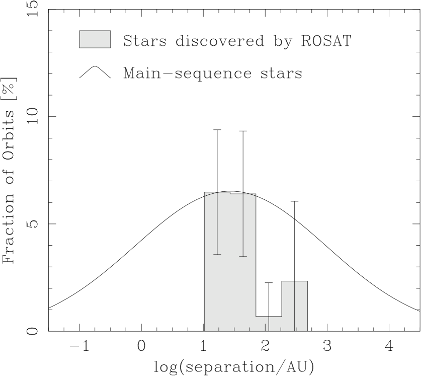
Figure 7: Companion star frequency as a function of projected separation. The histogram shows the result of this work, the curve shows the distribution of separations for main-sequence binaries. This is the result of a simulation for system masses of $1\rm\,M_{\sun}$, as described in section 5.1.

Fig. 7 shows the distribution of projected separations of the stars in our sample and main-sequence stars. The companion star frequencies in the range 10 – 70 AU agree almost perfectly, but at larger separations, the number of companions to young stars drops to nearly zero and is significantly lower than the number of companions to main-sequence stars. A Kolmogorov-Smirnov test shows that the two distributions are indeed different: the probability that both samples were drawn from the same distribution is only $6\cdot 10^{-6}$. The separation distribution of young stars in Chamaeleon appears to be more similar to that of low-mass stars in the Orion Trapezium Cluster: a number of binaries with small separations that is comparable to main-sequence stars (Prosser et al., 1994; Padgett et al., 1997; Petr et al., 1998), and only a very small number of binaries at larger separations (Scally et al., 1999).

Table 3: Companion star frequencies

	Main-sequence	All Stars in	PMS	ZAMS	Unknown
	Stars	Our Sample			Evol. Status
Total	164	77	33	4	40
Companions		$11.3\pm 3.9$	$\phantom{0}5.4\pm 2.6$	$\phantom{0}0.8\pm\phantom{0}1.0$	$\phantom{0}5.0\pm 2.6$
Companions per 100 systems	$24.1\pm 3.8$	$14.7\pm 5.1$	$16.3\pm 8.0$	$20.1\pm 25.0$	$12.6\pm 6.6$

5.4 Stars of different evolutionary status

Covino et al. (1997) used high-resolution spectra to classify ROSAT-selected stars in Chamaeleon as PMS star, ZAMS star, or star of unknown evolutionary status. Their object list is only a subset of our sample; we treat stars not observed by them as stars of unknown evolutionary status. Table 3 shows the results of our multiplicity survey for the different classes. Due to the large errors caused by the small sample size, we are unable to find a significant difference between stars of different evolutionary status.

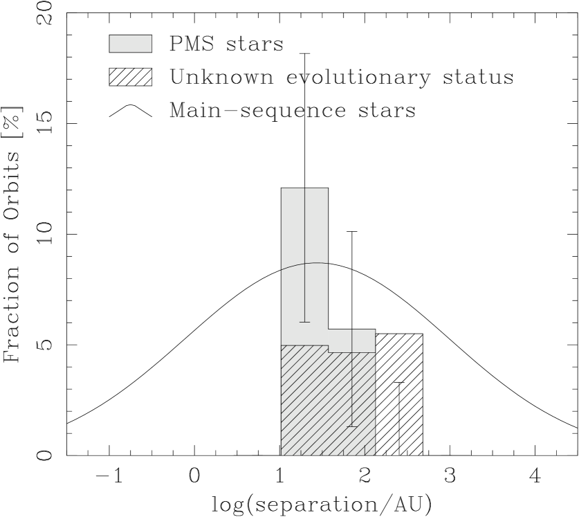
Figure 8: The distributions of projected separations of PMS stars and stars of unknown evolutionary status. Only error bars for PMS stars are shown to enhance the clarity of the diagram.

Figure 8 shows the distribution of separations of PMS stars and stars of unknown evolutionary status (it would not be useful to plot the one ZAMS binary). The bias towards binaries with small separations appears to be even more pronounced among bona-fide PMS stars, while the distribution of presumably older stars is more or less flat. We take this as an indication that the unusual distribution of separations we found for the whole sample is indeed a feature of the ROSAT-selected PMS stars in this region.

A KS test gave a probability of 38 % that the distributions of PMS stars and of stars of unknown evolutionary status were drawn from the same parent distribution. This result does not enable us to accept or reject the hypothesis that both distributions are identical. The sample of stars of unknown evolutionary status is probably a mixture of PMS and older stars. It shows a separation distribution that is similar to main-sequence stars, albeit with a smaller total number of companions.

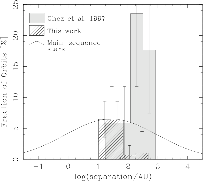
Figure 9: The distributions of projected separations of stars observed by Ghez et al. (1997) and in this work.

5.5 Comparison to Ghez et al. (1997)

Ghez et al. (1997) conducted a multiplicity speckle survey of TTS in southern star-forming regions known before ROSAT, including stars in the Chamaeleon star-forming region. The sensitivity of their observations for faint companions is rather non-uniform, but the observations of 17 stars in Chamaeleon have a sensitivity comparable to our observations. We assumed a distance of 160 pc for these stars, since the majority is located in the Cha I complex.

Figure 9 shows the distribution of projected separations of the stars observed by Ghez et al. (1997) compared to the stars observed by us. The distributions are clearly different. A $\chi^{2}$ test confirms this, the probability that both samples were drawn from the same distribution is only $10^{-11}$, a KS test gave a probability of 2.4 %. This difference cannot be explained by errors in the distances. To bring the peaks of both distributions together, the distance to one of the groups would have to be changed by a factor of 10.

This indicates that both samples represent two different populations of stars. This is not very surprising, since the distances of the two groups differ by a factor of two (see section 5.2). However, observations of other star-forming regions have shown that regions with a higher stellar density contain fewer binaries (Petr et al., 1998; Duchêne et al., 1999). In Chamaeleon, we find the opposite trend: the stars observed by Ghez et al. (1997) are located in the dense cores, yet their binary frequency is lower.

There are two possible explanations for this result: either the dependence of the binary frequency on the environmental conditions is not a simple function of stellar density, or the ROSAT-selected stars in Chamaeleon formed in a much denser environment. The proper motions of 31 of the ROSAT-selected stars are known (Frink et al., 1998; Frink, 1999). Their proper motion vectors are not oriented away from a single point, so they show no sign that the distribution was more concentrated in the past.

It is more likely that the stars formed near their present location in small “cloudlets” (Feigelson, 1996). Such small clouds have been discovered in a ${}^{13}{\rm CO}\,(J=1$–$0)$ survey by Mizuno et al. (1998). They found that about 70 % of the TTS in the region surveyed are located within 4 pc of a small cloud. However, it is not clear why only a small number of binaries formed in the cloudlets towards Chamaeleon, while under similar conditions in Taurus-Auriga most stars formed in binary systems.

6 Summary and Conclusions

We conducted a multiplicity survey of some 80 X-ray selected young stars. More than 50 % of them have been confirmed to be pre-main-sequence objects by measuring their Lithium abundances with the help of high-resolution spectroscopy (Covino et al., 1997). We find a companion star frequency that is lower by a factor of $0.61\pm 0.27$ compared to solar-type main-sequence stars (Duquennoy & Mayor, 1991). The separation distributions are remarkably different: We find almost no binaries among the young stars with separations larger than 100 AU.

The binary frequency and separation distribution of the confirmed pre-main-sequence stars are similar to that of the entire sample, although with a smaller statistical significance due to the smaller number of systems.

In contrast to our results for X-ray selected stars, Ghez et al. (1997) found a much higher binary frequency among 17 stars known before ROSAT. Our interpretation of this discrepancy is that the two samples represent two different populations. This agrees with the distance determinations, which indicate that at least some of the X-ray-selected stars are only half as distant as the stars known before ROSAT.

It remains unclear how the stars formed. According to the theory that the multiplicity depends on the stellar density, the small number of binaries and the shape of their separation distribution indicate that the stars were once in a much denser environment. However, the proper motions show no sign of expansion from a single point. This supports the hypothesis that the stars formed in small cloudlets at their present location (Feigelson, 1996; Mizuno et al., 1998), although we currently cannot explain the bias against wide binaries.

References

- Alcalá et al. (1995) Alcalá, J. M., Krautter, J., Schmitt, J. H. M. M., Covino, E., Wichmann, R., & Mundt, R. 1995, A&A Suppl. Ser. 114, 109
- Alcalá et al. (1997) Alcalá, J. M., Krautter, J., Covino, E., Neuhäuser, R., Schmitt, J. H. M. M., & Wichmann, R. 1997, A&A 319, 184
- Bouvier et al. (1997) Bouvier, J., Rigaut, F., & Nadeau, D. 1997, A&A 323, 139
- Brandner et al. (1996) Brandner, W., Alcalá, J. M., Kunkel, M., Moneti, A., & Zinnecker, H. 1996, A&A 307, 121
- Brandner & Köhler (1998) Brandner, W., & Köhler, R. 1998, ApJ 499, L79
- Briceño et al. (1997) Briceño, C., Hartmann, L. W., Stauffer, J. R., Gagné, M., Stern, R. A., Caillault, J.-P. 1997, AJ 113, 740
- Covino et al. (1997) Covino, E., Alcalá, J. M., Allain, S., Bouvier, J., Terranegra, L., & Krautter, J. 1997, A&A 328, 187
- Duchêne et al. (1999) Duchêne, G., Bouvier, J., & Simon, T. 1999, A&A 343, 831
- Duquennoy & Mayor (1991) Duquennoy, A., & Mayor, M. 1991, A&A 248, 455
- Durisen & Sterzik (1994) Durisen, R. H., & Sterzik, M. F. 1994, A&A 286, 84
- ESA (1997) ESA 1997, The HIPPARCOS Catalog, ESA SP-1200
- Feigelson (1996) Feigelson, E. D. 1996, ApJ 468, 306
- Frink et al. (1998) Frink, S., Röser, S., Alcalá, J. M., Covino, E., & Brandner, W. 1998, A&A 338, 442
-
Frink (1999)
Frink, S. 1999, Ph.D. Thesis, Ruprecht-Karls-Universität
Heidelberg, available at:
http://www.ub.uni-heidelberg.de/archiv/1100 - Ghez et al. (1993) Ghez, A. M., Neugebauer, G., & Matthews, K. 1993, AJ 106, 2005
- Ghez et al. (1997) Ghez, A. M., McCarthy, D. W., Patience, J., & Beck, T., 1997, AJ 481, 378
- Hofmann et al. (1992) Hofmann, R., Blietz, M., Duhoux, Ph., Eckart, A., Krabbe, A., & Rotaciuc, V. 1992, in Progress in Telescope and Instrumentation Technologies, ESO Conference and Workshop Proceedings No. 42, ed. M.-H. Ulrich M.-H. (Garching: ESO), 617
- Knox & Thompson (1974) Knox, K. T., & Thompson, B. J. 1974, ApJ 193, L45
- Köhler & Leinert (1998) Köhler, R., & Leinert, Ch. 1998, A&A 331, 977
- Köhler et al. (2000) Köhler, R., Kunkel, M., Leinert, Ch., & Zinnecker, H. 2000, A&A 356, 541
- Köhler (2001) Köhler, R. 2001, in Young Stars Near Earth: Progress and Prospects, ed. R. Jayawardhana & T. Greene (San Francisco: ASP)
- Kroupa (1995a) Kroupa, P. 1995, MNRAS 277, 1491
- Kroupa (1995b) Kroupa, P. 1995, MNRAS 277, 1522
- Leinert (1992) Leinert, Ch. 1992, in Star Formation and Techniques in Infrared and mm-Wave Astronomy, Proceedings of the European Astrophysical Doctoral Network Summer School V, ed. T. P. Ray, S. Beckwith, (New York: Springer)
- Leinert et al. (1993) Leinert, Ch., Zinnecker, H., Weitzel, N., Christou, J., Ridgway, S. T., Jameson, R., Haas, M., & Lenzen, R. 1993, A&A 278, 129
- Leinert et al. (1997) Leinert, Ch., Henry, T., Glindemann, A., & McCarthy, D. W. 1997, A&A 325, 159
- Lohmann et al. (1983) Lohmann, A. W., Weigelt, G., & Wirnitzer, B. 1983, Appl. Opt., 22, 4028
- Mamajek et al. (1999) Mamajek, E. E., Lawson, W. A., & Feigelson, E. D. 1999, ApJ 516, L77
- Mizuno et al. (1998) Mizuno, A., Hayakawa, T., Yamaguchi, N., Kato, S., Hara, A., Mizuno, N., Yonekura, Y., Onishi, T., Kawamura, A., Tachihara, K., Obayashi, A., Xiao, K., Ogawa, H., & Fukui, Y. 1998, ApJ 507, L83
- Neuhäuser et al. (1995) Neuhäuser, R., Sterzik, M. F., Schmitt, J. H. M. M., Wichmann, R., Krautter, J. 1995, A&A 295, L5
- Neuhäuser & Brandner (1998) Neuhäuser, R. & Brandner, W. 1998, A&A 330, L29
- Padgett et al. (1997) Padgett, D. L., Strom, S. E., & Ghez, A. 1997, ApJ 477, 705
- Petr et al. (1998) Petr, M. G., Coudé du Foresto, V., Beckwith, S. V. W., Richichi, A., & McCaughrean, M. J. 1998, ApJ 500, 825
- Press et al. (1994) Press, W. H., Teukolsky, S. A., Vetterling, W. T., & Flannery, B. P. 1994, Numerical Recipes in C, 2nd Ed., (Cambridge University Press)
- Prosser et al. (1994) Prosser, C. F., Stauffer, J. R., Hartmann, L., Soderblom, D. R., Jones, B. F., Werner, M. W., & McCaughrean, M. J. 1994, ApJ 421, 517
- Reipurth & Zinnecker (1993) Reipurth B., & Zinnecker, H. 1993, A&A 278, 81
- Scally et al. (1999) Scally, A., Clarke, C., & McCaughrean, M. J. 1999, MNRAS, 306, 253
- Schwartz (1991) Schwartz, R. D., in Low Mass Star Formation in Southern Molecular Clouds, ESO Report No. 11, ed. B. Reipurth B., 93
- Walter et al. (1988) Walter, F. M., Brown, A., Mathieu, R. D., Myers, P. C., Vrba, F. J. 1988, AJ 96, 297
- Wichmann et al. (1998) Wichmann, R., Bastian, U., Krautter, J., Jankovics, I., & Rucinski, S. M. 1998, MNRAS 301, 39L