BLOB EJECTION FROM ADVECTION-DOMINATED ACCRETION FLOW II: THE MULTIWAVELENGTH PROPERTIES OF LIGHT CURVES

Abstract

It has been argued that blobs ejected from advection-dominated accretion flow through the accretion-ejection instability undergo expansion due to their high internal energy density. The expanding blobs interact with their surroundings and form strong shock, which accelerates a group of electrons to be relativistic. Then flares are formed. This model has advances in two aspects: shock acceleration and self-consistent injection. We derive an analytical formula of the injection function of relativistic electrons based on the Sedov’s law. We calculate the time-dependent spectrum of relativistic electrons in such an expanding blob. The light-travel effect, the evolution of the electron spectrum due to energy loss, and the escape of relativistic electrons from the radiating region are considered, as well as the expansion (at sub-relativistic speed) of the coasting blob. A large number of light curves spanning wide spaces of parameters have been given in this paper. Regarding the symmetry, relative amplitude, duration of a flare, and the time lag between peak fluxes, we find four basic kinds of light curves for the non-expanding blob, and seven basic kinds of light curves for the expanding blob. The expansion weakens the magnetic field as well as enlarges the size of the blob. The predicted light curves thus show very complicated properties which are composed of the basic light curves, because the physical conditions are changing in the expanding blob. For the rapid decays of magnetic filed (for example, $B\propto r^{-n}$), we find the falling profile is a power law of time as $\nu F_{\nu}\propto t^{(1-\alpha)n/5}$, where $\alpha$ is the power-law index of injected electrons. This decline is controlled by the decay of magnetic field rather than the energy losses of relativistic electrons. We also calculate the evolution of the photon spectrum from both non-expanding and expanding blobs. Different shapes in the phase of decreasing luminosity are then obtained for different parameter values. The photon index, $\alpha_{\rm ph}$, keeps constant for non-expanding blobs when luminosity decreases, whereas $\alpha_{\rm ph}$ continues to decrease after the luminosity reaches its maximum for expanding blobs. It is expected that we can extract the information of ejected blobs from the observed light curves based on the present model.

1. Introduction

The time variations of received fluxes and emission spectra of blazar-type active galactic nuclei (AGNs) have received great attention from both theory and observation during the last 30 years, because the multiwavelength observations of flares from blazars provide invaluable information how the central engines work (Bregman 1990; Urry & Padovani 1995; Ulrich et al. 1997). The flare variabilities from blazars are very common. However, the properties of these flares are diverse, and the outbursts of the flares are over multiwavelength. Although we have a plenty of observational data of these phenomena, our understanding of the mechanisms of the flares are still insufficient.

Many attempts have been made to fit the observed continuum spectra by varieties of theoretical models. These calculations can be mainly divided into two kinds: homogeneous models (blob models) and inhomogeneous models (elongated jet models). At early stage the homogeneous models were frequently invoked owing to their concise physical scenario. Rees (1966, 1967) and Ozernoy & Sazonov (1968) originally studied the emergent spectrum from an expanding blob disregarding the evolution of the electron spectrum and blob dynamics. Subsequently, the expanding process was studied (Mathews 1971; Vitello & Salvati 1976; Canuto & Tsiang 1977; Christiansen, Scott, & Vestrand 1978). The free expanding case was considered under the assumptions that the electron spectrum is steady without time evolution (Jones & Tobin 1977; Vitello & Pacini 1977 and 1978; Königl 1978; Marscher 1980; Band & Grindlay 1986). Then the effect of electron spectrum evolution with presumed injection function was generally considered (Celotti, Maraschi, & Treves 1991; Wang & Zhou 1995; Mastichiadis & Kirk 1997; Kirk, Rieger, & Mastichiadis 1998; Dermer, Sturner, & Schlickeiser 1997; Dermer 1998; Georganopoulos & Marscher 1998; Chiaberge & Ghisellini 1999; Li & Kusunose 2000; Kusunose, Takahara, & Li 2000). The random fluctuations of the continuum from blazars are generally attributed to the propagation of relativistic shock (Marscher & Gear 1985). Large flares most probably result from a blob (Dermer, Sturner, & Schlickeiser 1997; Chiaberge & Ghisellini 1999) as considered by the authors listed above. It should be cautioned that all the calculations avoid three important processes: 1) how to accelerate the electrons in the blob, 2) how to inject the accelerated electrons into the blob if radiation regions are separated from acceleration regions, and 3) why and how to eject a blob. It is generally believed that these problems are related with accretion disks around supper massive black holes as a central engine. The status of accretion disks may determine the properties of the ejected blobs.

The properties of the iron K$\alpha$ line emission in radio-loud quasars may provide a new clue to understand the flare process, because it is a powerful probe to test the ionization state of matter close to black holes. The available data show that the line profiles in radio-loud quasars are very narrow (Sambruna et al. 1999; Reeves & Turner 2000), which are quite different from radio-quiet quasars and Seyfert galaxies. Thus an optically thin advection-dominated accretion flow (ADAF, Narayan & Yi 1994) or ion-pressure supported tori (Rees et al. 1982) may power the central engine in radio-loud quasars, which may be explained by the properties of iron K$\alpha$ line (Sambruna et al. 1999). If the accretion powers the central engine, then the accretion rate is roughly of order

$$\dot{m}\sim 10^{-3}{\cal D}_{10}^{-4}L_{47}M_{8}\,,$$ (1)

where $\dot{m}$ is the dimensionless accretion rate normalized by the Eddington rate, ${\cal D}_{10}$ is the Doppler factor normalized by 10, i.e., ${\cal D}_{10}={\cal D}/10$, $L_{47}$ is the bolometric luminosity normalized by $10^{47}$ erg/s, i.e., $L_{47}=L_{\rm bol}/10^{47}$, and $M_{8}$ is the black hole mass normalized by $10^{8}M_{\sun}$, i.e., $M_{8}=M_{\rm BH}/(10^{8}M_{\sun})$. Such a crude estimation is in agreement with that $\dot{m}\sim 10^{-2\sim-3}$ in FRII galaxies evaluated by Ghisellini & Celotti (2001). Indeed, such a low accretion rate implies that optically thin ADAF or ion-pressure supported tori may power the central engine. The observed bolometric luminosity suggests that the emission regions are highly relativistically boosted, which dominates over the emission from accretion disks (or ion-pressure supported tori).

Tagger & Pellat (1999) showed there is a strong accretion-ejection instability, which increases with the height of an accretion disk. Based on this instability, Wang et al. (2000) suggested that there is a large flare if a blob ejection takes place in optically thin ADAF of blazars. Comparing with the blob’s surroundings, Wang et al. (2000) also suggested the observational consequences of an ejected blob: nonthermal flares and recombination line emission, which are caused by the expansion of a blob owing to its high internal energy density. In fact there is an ample of evidence for the blob ejection from the nucleus. Especially, recent observations of 3C 273 by Chandra discovered the blob ejection from the central region (Marshall et al. 2001). If the flare arises from blob ejection, according to the model of Wang et al. (2000), what are the properties of the ejected blob in multiwavelength continuum? It is the goal of our paper to calculate the multiwavelength light curves of the emission from the ejected blob.

This paper is arranged as follows. Section 2 describes our model and the formulation, and an analytical injection function is derived from Sedov’s self-similar expansion. Extensive qualitative analyses of light curves are given in §3. To compare with observations we provide a large number of light curves and confirm the qualitative analysis in §4. Discussions and conclusions are given in the last section.

2. The descriptions of models

Supposing that the inter-cloud medium is homogeneous, the expansion of a blob is quite similar to the $\gamma$-ray burst fireball. As shown by Wang et al. (2000) the expansion is sub-relativistic. The expansion leads to the formation of strong shock. Thus such an expansion can be described by the self-similar solution after the timescale $t_{1}$ (Sedov 1969), which is rather shorter than that of the expansion phase. Sedov (1969) gives the self-similar solution: the shock speed $v_{\rm sh}\propto t^{-3/5}$ and shell radius $r_{\rm sh}\propto t^{2/5}$. Some electrons in the swept medium by blob expansion will be accelerated to be relativistic. Therefore, the expansion acts as the injection of relativistic electrons. We follow the usual assumption that a power-law distribution ($\gamma^{-\alpha}$) of electrons is formed via shock acceleration, where $\gamma$ is the Lorentz factor of an electron. The acceleration timescale is assumed to be much shorter than the expansion and synchrotron timescales (for the acceleration timescale, e.g., Kirk et al. 1994 and references therein). Then the injection function $Q(\gamma,t)$ can be written as $Q(\gamma,t)\propto r_{\rm sh}^{2}v_{\rm sh}\propto t^{1/5}$. Because the expansion of the blob will be drastically decelerated after long enough time, we introduce a cutoff factor $e^{-t/t_{2}}$,

$$Q(\gamma,t)=Q_{0}\gamma^{-\alpha}t^{1/5}e^{-t/t_{2}}\,,$$ (2)

where $Q_{0}$ can be obtained by the total injected energy $E_{0}$ after integrating the time and electron energy,

$$Q_{0}\approx\frac{6(2-\alpha)E_{0}}{5m_{e}c^{2}\left[(\gamma^{0}_{\rm max})^{2-\alpha}-(\gamma^{0}_{\rm min})^{2-\alpha}\right]t_{2}^{6/5}},~{}~{}~{}{\rm for}~{}~{}\alpha\neq 2\,.$$ (3)

For $\alpha=2$, we have $Q_{0}\approx 6E_{0}/[5m_{e}c^{2}t_{2}^{6/5}\ln(\gamma_{\rm max}/\gamma_{\rm min})]$. Equation (2) implies that the injection is roughly constant within a timescale $t_{2}$. The evolution of electron energy can be determined by $\gamma=\gamma_{0}/(1+a\gamma_{0}t)$, where $\gamma_{0}$ is the initial energy of electron and $a=c\sigma_{\rm T}B^{2}/6\pi m_{e}c^{2}=1.29\times 10^{-9}B^{2}$. Here $c$ is the light speed, $\sigma_{\rm T}$ is the Thomson cross section, $m_{e}$ is the electron mass, and $B$ is the magnetic field strength in units of Gauss. The electron continuity equation in the homogeneous expanding blob reads

$$\frac{\partial N(\gamma,t)}{\partial t}+\frac{\partial}{\partial\gamma}\left[b(\gamma)N(\gamma,t)\right]+\frac{N(\gamma,t)}{\tau_{\rm esc}}=Q(\gamma,t)\,,$$ (4)

where $b(\gamma)=-a\gamma^{2}$ and $\tau_{\rm esc}$ is the timescale of electron escape from the radiation region, which determines the later evolution of a flare showing up in lower frequencies. If re-acceleration of relativistic electrons takes place the pile-up distribution will be formed in the shell (Schlickeiser 1984), but we neglect the re-acceleration here. Therefore the solution of the continuity equation of electrons is given by (Ginzburg & Syrovatskii 1965)

$$N(\gamma,t)=\frac{1}{b(\gamma)}\int_{\gamma}^{\gamma_{\rm max}}\exp\left(-\frac{\tau}{\tau_{\rm esc}}\right)Q(\gamma_{0},t-\tau)d\gamma_{0}\,,$$ (5)

where $\tau=\int_{\gamma_{0}}^{\gamma}b^{-1}(\gamma^{\prime})d\gamma^{\prime}=\left(\gamma^{-1}-\gamma_{0}^{-1}\right)/a$. The number density of the electrons reads $n(\gamma,t)=N(\gamma,t)/(4\pi r^{2}_{\rm sh}\Delta r_{\rm sh})$. These equations describe the evolution of the relativistic electrons.

It is known that the observed light curve is “contaminated” by two factors: the size of a blob and the evolution of the relativistic electrons. Therefore the information of geometric structure and motion is hidden in the light curves as well as the pure evolution of electrons. Figure 1 shows the geometry of the expanding blob in its coasting frame. Suppose at a given time $t_{\rm blob}$ (in the blob frame), the location of its center is $C^{\prime}$, and the distance to the observer is $d_{\rm o^{\prime}c^{\prime}}$. For the arbitrary point $P(r_{\rm sh},\theta^{\prime},\phi^{\prime})$ on the shell, the distance of $P$ to the observer reads

$$d_{{}_{\small{\rm O^{\prime}P}}}\approx d_{{}_{\small{\rm O^{\prime}C^{\prime}}}}\left[1-\left(\frac{r_{\rm sh}}{d_{{}_{\small{\rm O^{\prime}C^{\prime}}}}}\right)\cos\psi\right]\,,$$ (6)

where $\cos\psi=\sin\theta^{\prime}\sin(\phi^{\prime}+\Theta)$, $\psi$ is angle PC^′O^′, and $\Theta$ is the angle between the line of sight and the motion of the blob. This approximation is always valid because of $d_{\rm o^{\prime}c^{\prime}}\gg r_{\rm sh}$. Here we neglect the change of angle $\Theta$ due to the motion of the blob, because the distance of the blob is so far away from the observer. It is pointed out that we compare the observer time $t_{\rm obs}$ with the time at the center of the blob $t_{b}^{\prime}$, i.e., $t_{\rm obs}=t_{b}^{\prime}/{\cal D}$, where $\cal{D}$ is the Doppler factor given by ${\cal{D}}=1/\Gamma(1-\beta\cos\Theta)$, with $\Gamma$ being the Lorentz factor of the blob motion and $\beta=(1-1/\Gamma^{2})^{1/2}$. Then we can set up the relation between radiation time $t^{\prime}$ (time at $P$) and the blob time at the center:

$$t^{\prime}=t_{\rm b}^{\prime}+\frac{d_{{}_{\small{\rm O^{\prime}C^{\prime}}}}-d_{{}_{\small{\rm O^{\prime}P}}}}{c}\approx t_{\rm b}^{\prime}+\left(\frac{r_{\rm sh}}{c}\right)\cos\psi\,,$$ (7)

with sufficient accuracy. The retardation is clear in this equation. The shell thickness $\Delta r_{\rm sh}$ increases with the radius of the blob, but $\Delta r_{\rm sh}/r_{\rm sh}\ll 1$ holds for the expansion phase (Sedov 1969). Thus our treatments are valid.

The synchrotron emissivity of relativistic electrons is denoted by $\epsilon_{\nu}$, then the emission from a shell element $(\Delta r_{\rm sh},\Delta\theta^{\prime},\Delta\phi^{\prime})$ should be $\Delta L_{\nu}=\epsilon_{\nu}(r^{2}_{\rm sh}\Delta r_{\rm sh})\sin\theta^{\prime}\Delta\theta^{\prime}\Delta\phi^{\prime}$, where $\epsilon_{\nu}(t)=c_{3}B\int_{\gamma_{\rm min}}^{\gamma_{\rm max}}n(\gamma,t)F(x)dx$, $x=\nu/\nu_{0}B\gamma^{2}$, $F(x)=x\int_{x}^{\infty}K_{5/3}(z)dz$, and $K_{5/3}$ is the modified Bessel function with order 5/3, $\nu_{0}=3e/4\pi m_{e}c=4.21\times 10^{6}$, and $c_{3}=\sqrt{3}e^{3}/(4\pi m_{e}c^{2})=1.87\times 10^{-23}$ (Pacholczyk 1973). The blob is optically thin in our interested bands, which are much higher than the synchrotron self-absorption frequency. The emergent spectrum from the shell of the expanding blob can be written as

$$L(\nu^{\prime},t_{\rm b}^{\prime})=c_{3}B\int_{0}^{\pi}\sin\theta^{\prime}d\theta^{\prime}\int_{0}^{2\pi}d\phi^{\prime}\int_{\gamma_{2}}^{\gamma_{1}}H(\zeta)N(\gamma,t^{\prime})F(x)d\gamma\,,$$ (8)

where $H(\zeta)$ is the Heaviside function: $H(\zeta)=0$ for $\zeta<0$, whereas $H(\zeta)=1$ for $\zeta\geq 0$. Here parameter $\zeta$ is given by

$$\zeta=t_{\rm b}^{\prime}+\frac{r_{\rm sh}}{c}\cos\psi\geq 0\,,$$ (9)

which is incorporated from equations (6) and (7). The introduction of the Heaviside function is based on the retardation of light propagation. Because of the infinitesimal thickness of the shell, the retardation of photons to the observer is caused only by emission from different points ($\theta^{\prime}$, $\phi^{\prime}$). It is interesting to note that the emission (eq. 8) is independent of the specific geometric thickness of the shock. This leads to the avoidance of the discussion of the shock thickness.

We assume the magnetic field changes with radius as

$$B(r)=B_{0}\left(\frac{r}{r_{\rm sh}^{0}}\right)^{-n},$$ (10)

where $r_{\rm sh}^{0}$ is the radius of blob at $t=t_{1}$. The index $n$ remains a free parameter in our model. The flux from the whole blob received by a distant observer is obtained by Lorentz transformation as

$$F({\nu},t_{\rm obs})=\frac{1}{4\pi d_{L}^{2}}{\cal D}^{3}L\left(\frac{\nu}{\cal{D}},{\cal D}t_{\rm obs}\right)\,,$$ (11)

where $d_{L}$ is the luminosity distance from the source to the observer. Here we neglect the difference in the directions of emitting locations in the blob measured from the line of sight. Also for simplicity we neglect the difference of Doppler factor at different locations in the blob, because the expansion is sub-relativistic.

As a summary of the parameters employed in the present model, all of them are listed in Table 1. There are 12 parameters describing the processes in the blob. Some of them are the initial values of the blob, for example, $B_{0}$, $r_{\rm sh}^{0}$, and $\beta_{0}$. With the help of Sedov self-similar solution, these parameters at any time will be known. The escape timescale is taken to be a free parameter. The dependence of magnetic field on the shell radius owing to expansion is an adjustable parameter. The timescale of injection $t_{2}$ is a new parameter, and $t_{1}$ in fact connects with the initial expansion velocity $\beta_{0}$ (eq. 23 below). For a non-expanding blob there are 11 parameters (1 – 11). The non-expanding blob in fact is homogeneous for a distant observer, whereas the expanding blob shows the inhomogeneous properties as we show below.

3. Qualitative analysis

Generally speaking there are four aspects to describe the characteristics of the light curves at different wavebands: 1) the symmetry of light curves about the peak flux, 2) the relative amplitudes of light curves at the peaks, 3) duration of the bursts, which is defined by the $e$-folding time of $\nu F_{\nu}$, 4) the time lag of the light curves, which is defined as the time interval between the peak fluxes at different wavebands. Sophisticated observations should discover these properties by comparing observed spectra with the theoretical models.

From equation (8) we know that there are four processes affecting the observed light curves: blob’s expansion which increases the blob’s size, energy losses of electrons via synchrotron radiation, photon traveling, and the escape of electrons from the blob shell. The four processes are competing each other, determining the properties of light curves, and are hidden in the observed light curves. We first analyze the roles of the size, escape, and energy losses in the light curves before making detailed numerical calculations.

3.1. Non-expansion cases

Considering the complexities of the expanding blobs, we first analyze the most simple cases of the non-expansion blobs. There are three important timescales, i.e., 1) $\tau_{\rm syn}$: energy loss timescale due to synchrotron radiation, which is proportional to $\nu^{-1/2}$, 2) $\tau_{\rm ltr}$: light-travel timescale through the blob, 3) $\tau_{\rm esc}$: the timescale of electron escape from the radiation region. Here we consider two light curves of photons with frequencies $\nu_{1}$ and $\nu_{2}$ ($\nu_{1}>\nu_{2}$). The lifetimes of relativistic electrons which radiate photons at frequencies $\nu_{1}$ and $\nu_{2}$ are denoted by $\tau_{\rm syn}^{\nu_{1}}$ and $\tau_{\rm syn}^{\nu_{2}}$, respectively. The total energy radiated at $\nu$ during lifetime $\tau_{\rm syn}^{\nu}\propto\gamma^{-1}$ is given by

$$\Delta E\sim\gamma N(\gamma,t)\propto\gamma^{1-\alpha}\,.$$ (12)

For $\nu_{1}$ and $\nu_{2}$, their total radiated energies are $\Delta E_{1}\propto\gamma_{1}^{1-\alpha}$ and $\Delta E_{2}\propto\gamma_{2}^{1-\alpha}$ within $\tau_{\rm syn}^{\nu_{1}}$ and $\tau_{\rm syn}^{\nu_{2}}$, respectively. Generally the size of the blob determines the duration of a flare, if $\tau_{\rm ltr}$ is long enough. The escape effect will sharpen the falling profile and the peak flux, if $\tau_{\rm esc}$ is short enough. The retardation of the peak flux at different bands is obviously determined by the above three processes in the blob, i.e., synchrotron loss, light travel, and electron escape. The competition among the three timescales determines the light curves from the blob. According to these timescales, we distinguish the following four kinds of light curves for a non-expanding blob.

(NE1) For the case of $\tau_{\rm syn}^{\nu_{1}}<\tau_{\rm syn}^{\nu_{2}}<\tau_{\rm ltr}\ll\tau_{\rm esc}$, energy loss timescales are shorter than $\tau_{\rm ltr}$ and much shorter than $\tau_{\rm esc}$. This implies that the escape can be neglected. Under such a circumstance, only one process, namely, light traveling, determines the observed light curves, because the lifetime of electrons is shorter than light travel timescale $\tau_{\rm ltr}$. Then the observed light curves are mainly due to the light travel effects. The light curves should be symmetric about the peak flux, because the rising time and the falling time are roughly equal to $\tau_{\rm ltr}$. The time lag may roughly be zero. The radiation processes of relativistic electrons will be hidden. The duration of the flare is roughly equal to light travel timescale $\tau_{\rm ltr}$, too. Now we define LC₁ and LC₂ as the light curves at frequencies $\nu_{1}$ and $\nu_{2}$, respectively. The peak fluxes of LC₁ and LC₂ are denoted by $L^{\rm pk}_{1}$ and $L^{\rm pk}_{2}$, respectively. Thus the ratio of the peak fluxes will be given by

$$\frac{L^{\rm pk}_{1}}{L^{\rm pk}_{2}}\sim\frac{\Delta E_{1}/\tau_{\rm ltr}}{\Delta E_{2}/\tau_{\rm ltr}}=\left(\frac{\gamma_{1}}{\gamma_{2}}\right)^{1-\alpha}=\left(\frac{\nu_{1}}{\nu_{2}}\right)^{(1-\alpha)/2},$$ (13)

from equation (12).

(NE2) For the case of $\tau_{\rm syn}^{\nu_{1}}<\tau_{\rm ltr}<\tau_{\rm syn}^{\nu_{2}}\ll\tau_{\rm esc}$. The longer timescale of escape guarantees the rough conservation of the number of radiating electrons in the blob. The light curve at frequency $\nu_{1}$, LC₁, is still determined by the blob’s geometry, but one at $\nu_{2}$, LC₂, will be determined by radiation processes and blob’s geometry. The rough symmetry remains in LC₁, whereas asymmetry in LC₂ appears. This is simply owing to the differences between rising timescale (due to light travel and energy losses) and falling timescale (due to radiation). The duration time of LC₁ will be determined by the light travel timescale $\tau_{\rm ltr}$, and the duration of LC₂ will be modulated by light travel timescale and radiation timescale $\tau_{\rm ltr}+\tau_{\rm syn}^{\nu_{2}}$. The time lag is controlled by synchrotron radiation and light travel. The duration of LC₁ is still determined by the blob’s size, but the duration of LC₂ will be roughly determined by synchrotron radiation. The ratio of the peak flux will be roughly given by

$$\frac{L^{\rm pk}_{1}}{L^{\rm pk}_{2}}\sim\frac{\Delta E_{1}/\tau_{\rm ltr}}{\Delta E_{2}/(\tau_{\rm ltr}+\tau_{\rm syn}^{\nu_{2}})}=\left(1+\frac{\tau_{\rm syn}^{\nu_{2}}}{\tau_{\rm ltr}}\right)\left(\frac{\nu_{1}}{\nu_{2}}\right)^{(1-\alpha)/2}\,,$$ (14)

implying the combined effects of the spectrum, size, and magnetic field.

(NE3) For the case of $\tau_{\rm ltr}<\tau_{\rm syn}^{\nu_{1}}<\tau_{\rm syn}^{\nu_{2}}\ll\tau_{\rm esc}$. The shortest timescale is the travel timescale, which means that the blob’s geometry is less important in the light curves. The time lag is caused by the differences of energy-loss timescales at $\nu_{1}$ and $\nu_{2}$. The retardation of the flux peak will be of order

$$\tau_{\rm lag}\sim\tau_{\rm syn}^{\nu_{2}}-\tau_{\rm syn}^{\nu_{1}}\,.$$ (15)

The ratio of the amplitudes is determined by the spectrum of relativistic electrons, roughly given by

$$\frac{L^{\rm pk}_{1}}{L^{\rm pk}_{2}}\sim\frac{\Delta E_{1}/\tau_{\rm syn}^{\nu_{1}}}{\Delta E_{2}/\tau_{\rm syn}^{\nu_{2}}}=\left(\frac{\nu_{1}}{\nu_{2}}\right)^{(2-\alpha)/2}\,.$$ (16)

The duration of a flare is mainly determined by the lifetime of electrons radiating at this frequency, which can be roughly expressed by $\tau_{\rm syn}^{\nu_{1}}/\tau_{\rm syn}^{\nu_{2}}\sim(\nu_{2}/\nu_{1})^{-1/2}$. The profile of light curves may be asymmetric, because the rising timescale is determined by the injection, and the falling timescale is determined by energy losses.

(NE4) The case of $\tau_{\rm syn}^{\nu_{1}}<\tau_{\rm esc}<\tau_{\rm syn}^{\nu_{2}}<\tau_{\rm ltr}$. The above three cases are presumed that the escape timescale is much longer than any other timescales. This assumption guarantees the conservation of electron number during the whole lifetime of relativistic electrons. The escape effects result in the decrease of the electron number (see Eq. 5). Equivalently, the total luminosity will be lowered. Now we consider an example of electron escape. In such a case the escape and light travel effects are important in the light curves. If the escape timescale of electrons is shorter than light travel and synchrotron radiation timescales, the case will be meaningless in observations, because the light curves are mainly determined by the escape process. On the other hand, if $\tau_{\rm syn}^{\nu_{1}}<\tau_{\rm esc}<\tau_{\rm syn}^{\nu_{2}}<\tau_{\rm ltr}$ holds, the ratio of the amplitudes will be given by

$$\frac{L^{\rm pk}_{1}}{L^{\rm pk}_{2}}\sim\frac{\Delta E_{1}/\tau_{\rm syn}^{\nu_{1}}}{\Delta E_{2}/\tau_{\rm esc}}=\frac{\tau_{\rm esc}}{\tau_{\rm syn}^{\nu_{1}}}\left(\frac{\nu_{1}}{\nu_{2}}\right)^{(1-\alpha)/2}\,,$$ (17)

which is controlled by the electron spectrum, escape, and magnetic field, and this case will be complicated. The rising profile of LC₂ is caused by synchrotron radiation, whereas its falling profile is by the escape process. The asymmetry appears in light curves, and the relative amplitude will be determined by escape and radiation processes.

The above discussions are summarized in Table 2, which gives the properties of light curves according to symmetry, duration, relative amplitude, and time lag. We rule out the case of $\tau_{\rm esc}<\min(\tau_{\rm ltr},\tau_{\rm syn}^{\nu_{1}},\tau_{\rm syn}^{\nu_{2}})$, because electrons will directly escape without emission.

3.2. Self-similar expansion

The expansion of a blob causes the light curves more complicated because of an additional timescale $\tau_{\rm exp}$. The light curves from an expanding blob will be given by the above four characteristic light curves with the modulations by expansion. Generally the expansion timescale is longer than that of the light travel timescale in the present model, because we are considering the non-relativistic expansion. Complexities arise from the changes of magnetic field and size of the blob due to expansion. Based on the four kinds of light curves described above, it is easy to distinguish the new characteristics of light curves from an expanding blob. We can compare the expansion timescale with the other three timescales; Table 2 is the summary of the meaningful light curves according to the four aspects of symmetry, duration, relative amplitude, and time lag.

The expansion not only enlarges the size of the blob, but also weakens the magnetic field. The enlarging size makes the light travel timescale longer; the weakening magnetic field dilates timescale of synchrotron emission but lowers the output emission power. From equation (10), we obtain the synchrotron timescale

$$\tau_{\rm syn}(\gamma)=\tau_{\rm syn}^{0}(\gamma)\left(\frac{r}{r_{\rm sh}^{0}}\right)^{2n}\,,$$ (18)

where $\tau_{\rm syn}^{0}=1.0\times 10^{9}/(\gamma B_{0}^{2})$ s, with $r_{\rm sh}^{0}$ and $B_{0}$ being the initial radius and magnetic field of the blob, respectively. For a mono-energetic electron with energy $\gamma$, the energy loss rate is given by

$$\dot{\gamma}(\gamma)=\dot{\gamma}_{0}(\gamma)\left(\frac{r}{r_{\rm sh}^{0}}\right)^{-2n},$$ (19)

and the peak frequency of its emission is

$$\nu_{\rm c}(\gamma)=\nu_{\rm c}^{0}(\gamma)\left(\frac{r}{r_{\rm sh}^{0}}\right)^{-n},$$ (20)

where $\dot{\gamma}_{0}=1.29\times 10^{-9}B_{0}^{2}\gamma^{2}$ and $\nu_{\rm c}(\gamma)=4.21\times 10^{6}\gamma^{2}B_{0}$ Hz. The index $n$ is between 1 and 2 for different models. From this equation we see that the synchrotron timescale is very sensitive to the expansion law of a blob. This makes the light curves very complicated, showing more than one kind of light curves in one flare.

Although the light curves behave similarly to those of the non-expanding blob, four timescales such as $\tau_{\rm syn}$, $\tau_{\rm ltr}$, $\tau_{\rm exp}$, and $\tau_{\rm esc}$ jointly control the light curves. Comparing them for the expanding blob, we obtain seven kinds of light curves and list them in Table 2 according to their basic properties such as symmetry, duration, relative amplitude and time lag.

4. QUANTITATIVE ANALYSIS

In this section we show our numerical results. As we already stressed, the present model includes the expansion effects through two processes of enlarging size and weakening magnetic field. We first show the results of a non-expanding blob, and then show the results of several cases for different parameters of an expanding blob, and last we compare the results of non-expanding and expanding blobs. We list all the cases for non-expansion and expansion in Tables 3 and 4, respectively. The photon energies are taken to be 0.1, 1, 10, 100 eV and 1, 2, 3, 4 keV, which span almost 5 orders of magnitude from near infrared, optical, UV, EUV, soft X-ray, to the middle range of X-ray bands. The Doppler factor is taken to be ${{\cal D}}=10$, and the total injection energy $E_{0}=10^{45}$ erg within time interval $t_{2}$. Also $\gamma_{\rm min}=10^{2}$ and $\gamma_{\rm max}=5\times 10^{5}$ are assumed in all models. Finally, $\Gamma=1/\Theta$ is assumed.

4.1. Electron energy spectra

Taking the form of equation (2) as the injection function, the electron energy spectrum can be obtained from equation (5). Here we should note that the injection function is based on Sedov’s self-similar solution and the evolution of the electron spectrum is self-consistent. Figures 2a and 2b show the electron spectra for two cases. For the non-expanding case, the number density increases with time for $t<t_{2}$. The increase is linear, because the injection rate is almost constant before time $t_{2}$. Another prominent characteristic is the break at high energy. This is due to cooling of synchrotron radiation. The difference in the spectral index between the low and high energy is unity. This will be reflected in the photon spectral energy spectrum as we show in the following figures of photon index evolution.

There are two possible cases for expansion cases. 1) The injection is faster than the energy losses. Since the synchrotron timescale is dependent on the electron energy, this condition will be satisfied for electrons with high energy in the late phase of the expansion by considering the magnetic field decays with time as $t^{2n/5}$. In such a case the number density will almost linearly increase with time. 2) Synchrotron loss is more rapid than expansion ($\tau_{\rm syn}<\tau_{\rm exp}$). Then the number density of high energy electrons will decrease, because the injection is too slow. Such a case may appear in the early phase of expansion, because the condition ($\tau_{\rm syn}<\tau_{\rm exp}$) will be satisfied. Then the spectral break will appear. In Figure 2b, the above two characteristics are evident: in the early phase there is a break due to energy losses, whereas in late phase the number density increases linearly and the break becomes weak. This will result in different behaviors in the plot of spectrum index versus luminosity in the later phase.

4.2. Non-expanding Blob

We now consider a non-expanding shocked shell of the blob in order to facilitate to compare with the expanding situations, although the non-expanding model may not operate in practice. Here we assume that the injection still takes the form of equation (2). The size and magnetic field hold constant. Therefore nine parameters are in the non-expansion model. Except $t_{2}$, other eight parameters are often used in homogeneous model, namely, the magnetic field $B$, Doppler factor ${\cal D}$, the injected total energy $E_{0}$, the index of the injected electron spectrum, the maximum and minimum Lorentz factors of the electron population, the size of the blob $r_{\rm sh}^{0}$, and the last is the timescale of electron escape from the radiation region.

In this model the most important timescale is the lifetime of electrons radiating synchrotron photons with $\nu$. The simple estimation of the lifetime is given by

$$\tau_{\rm syn}=2.0\times 10^{4}B^{-3/2}{\cal D}^{-1/2}\nu_{15}^{-1/2}~{}{\rm s},$$ (21)

where all the parameters are in observer’s frame, and $\nu_{15}=\nu/10^{15}$. The lifetime is insensitive to Doppler factor. We always keep the Doppler factor constant in various models. In this case the duration time, time lag, and relative amplitude of a flare in different bands will be independent of the total injected energy. Although there are other seven parameters in the simple homogeneous model, the key parameters are $r_{\rm sh}^{0}$, $B$, and $\tau_{\rm esc}$ which determine the duration time, the time lag, and the relative amplitudes in different bands. We show the details in Figs 3 – 7.

4.2.1 Size effects

Size effects are shown in Figure 3. We change the size as a free parameter and fix all other parameters. We take the size of the blob, $r_{\rm sh}$, to be $10^{15}$, $10^{16},5\times 10^{16}$, and $10^{17}$ cm to find the effects of the size on light curves.

Symmetry: The lowest panel in Figure 3 shows the light curves for $r_{\rm sh}=10^{17}$cm. It is interesting to find that the light curves in high energy bands (right panel) are symmetric about the peak, whereas the rising timescale is much shorter than the falling timescale in the low energy band (left panel). This quantitatively confirms the qualitative analysis in §3. The rising and falling timescales are determined by the light travel timescale $\tau_{\rm ltr}$ as we listed for high energy light curves in Table 2. This characteristic can be justified by comparing $\tau_{\rm ltr}$ and $\tau_{\rm syn}$. From the left panel, we see that the symmetry of light curves is gradually broken with the decrease of the size of the blob. We also see that the rising timescale decreases rapidly with $r_{\rm sh}$, because it is mainly determined by $\max(\tau_{\rm ltr},\tau_{\rm syn})$. Usually the rising time is shorter than the falling timescale for the asymmetric light curves. Other asymmetric light curves can be found in Figure 3 according to the condition listed in Table 2.

Duration ($\tau_{\rm d}$): We find the duration time is very sensitive to the size of a blob, because we defined the duration time as the $e$-folding time of $\nu F_{\nu}$. Generally $\tau_{\rm d}$ will be prolonged by the size. The duration time can be roughly given by $\tau_{\rm d}\sim\max(\tau_{\rm syn},\tau_{\rm ltr})$. The keV photons are radiated from electrons with high energy, and it is expected that $\tau_{\rm syn}<\tau_{\rm ltr}$. Thus $\tau_{\rm d}$ will be given by $\tau_{\rm ltr}$. From the figures in the left panel we find that $\tau_{\rm d}$ of lower energy photons is much longer than those in the right panel. The lower energy photons produced by electrons with lower energy, and it is expected that $\tau_{\rm syn}>\tau_{\rm ltr}$. Thus the duration time $\tau_{\rm d}$ will be mainly determined by $\tau_{\rm syn}$ as shown in the left panel, especially for the light curves of 0.1, 1, and 10eV photons. Table 2 lists the duration properties of LC₁ and LC₂ for the non-expansion cases.

Relative Amplitude: We find the light curves change with $r_{\rm sh}$ in several factors. First, for model A4, the condition of NE1 is satisfied; all the synchrotron timescales (for high energy light curves, see the right panel in Figure 3) are shorter than $\tau_{\rm ltr}$. The relative amplitudes are roughly approximated by equation (13). With the decrease in the blob size, the relative amplitudes for high energy light curves roughly keep constant but they become very complicated for low energy light curves, because the condition NE1 is broken. For model A2, $r_{\rm sh}=10^{15}$cm, $\tau_{\rm ltr}$ is shorter than any synchrotron timescales for lower energy light curves (left panel in Figure 3), then the condition NE3 is satisfied. The relative amplitudes are given by equation (16). The upper panel of the left side in Figure 3 indeed shows this property. Increasing the size, the relative amplitudes become complicated as shown for models A3, A1, and A4. Second, the peak flux decreases with the size, if condition NE1 is satisfied. This property can be seen from the right panel of Figure 3. The left panels show the relative amplitude of peaks at different bands non-monotonously decreases with the size for low energy light curves. This reflects the changes of conditions in the blob due to the size of blob. Third, the duration is generally prolonged with the increase in the size. All the three features can be explained by the fact that the changes of the size of a blob modify the light travel time. When the size is large enough for a fixed frequency, the broaden light curves will be of small amplitude, because the timescale of energy losses of electrons is long, which leads to the relative amplitudes of variations at lower frequency dominate over high frequency.

Time Lag: The most prominent properties of these light curves are the time lags among different wavebands. From Figure 3, we find $\tau_{\rm lag}$ is very sensitive to the size with complicated behaviors. For the symmetric light curves there is zero-lag ($\tau_{\rm lag}=0$), because the rising and falling timescales are given by $\tau_{\rm ltr}$ as for the case of $r_{\rm sh}=10^{17}$cm at 1, 2, 3, and 4keV wavebands. However for the asymmetric light curves, the time lag becomes complex. As we have already pointed out that the rising timescale is roughly determined by $\max(\tau_{\rm syn},\tau_{\rm ltr})$. Thus for high energy light curves the time lag $\tau_{\rm d}$ is mainly affected by the energy losses, if the size is small enough as shown by the right panel of Figure 3, which does not show significant time lag, because the rising timescale is too short to display by a large scale time axis. It is evident to find that time lags increase significantly with the size for lower energy light curves from the left panel of Figure 3. We still find time lags for $r_{\rm sh}=10^{15}$cm are too small to illustrate in Figure 3. Since $\tau_{\rm syn}>\tau_{\rm ltr}$ for 0.1, 1, and 10eV photons, it is expected that time lag is mainly determined by the synchrotron energy losses. For intermediate cases $\tau_{\rm d}$ will be jointly given by two processes, i.e., light travel and synchrotron radiation. Our numerical results confirm the qualitative analysis listed in Table 2.

Here we have addressed the effects of the blob’s size on the properties of light curves. These features are key observational implications, as we have shown and listed above in detail. Because the properties of light curves are highly dependent on the observable frequencies, it is desired to compare multiwavelength light curves.

4.2.2 Effects of magnetic fields

Equations (14), (16), and (17) already show the role of magnetic fields. The effects of magnetic field for the non-expansion cases are shown in Figure 4. We change the magnetic field as a free parameter, while all other parameters are fixed. The role of magnetic field can be deduced from the timescale of synchrotron losses $\tau_{\rm syn}\propto B^{-3/2}$ [equation (21)]. The stronger magnetic field, the shorter the timescale of synchrotron losses. This leads to 1) the luminosity is enhanced by increasing magnetic field, 2) the rising timescale becomes shorter if the size is small enough. We fix $r_{\rm sh}=10^{16}$cm and compare the model A1 with others to show the effects of magnetic field. Correspondingly, the peak flux reaches in advance by increasing the magnetic field. This leads to the shortening of time lag $\tau_{\rm lag}$. This can be directly seen in Figure 4. Of course the duration timescale $\tau_{\rm d}$ also shortens by increasing magnetic field. If the magnetic field is suitable, symmetric light curves will appear by combined effects of synchrotron losses and light travel. For $r_{\rm sh}=10^{16}$cm, we will obtain symmetric light curves, if we increase $B$ until $\tau_{\rm syn}<\tau_{\rm ltr}$.

4.2.3 Effects of electron energy index

Without a specific acceleration mechanism, we assume that the injection spectrum has a power-law with index $\alpha$. The equations in qualitative analysis indicate the importance of index $\alpha$. The roles of the power-law index $\alpha$ of the injected electrons are shown in Figure 5. From equation (3) we know that the lower energy electrons are dominant over high energy electrons, if $\alpha>2$. The power radiated in lower energy will be larger than that in high energy bands. This is already shown in Figure 3, where we take $\alpha=2.5$ in several models. Thus the contribution to the rising side of light curves due to the synchrotron radiation of electrons shifted from higher energy can be neglected, because its number is much less than the initial lower energy electrons. Time lag is very sensitive to the index $\alpha$. Lowering $\alpha$ leads to the postpone of the flux peak, and shortening time lag. The relative amplitude of peak fluxes decreases with the increase of $\alpha$. In such a case the relative amplitude of the peak fluxes would be related with the time lag.

4.2.4 Effects of electron escape

The role of escape of electrons from the radiation region is considered. It is easy to find from equations (5) and (17) that the number of electrons decreases with time. With the inclusion of the size effects, the escape have three factors: the vast decreases of fluxes, the shortening of time lag, and the asymmetry of light curves. These can be seen in Figure 6, where we fix the size of the blob as $r_{\rm sh}=10^{16}$cm. The escape effect is small on high energy light curves, because $\tau_{\rm syn}<\tau_{\rm esc}$. For the cases with longer escape timescale, its effects can be neglected. For example, $\tau_{\rm esc}/\tau_{\rm ltr}=20$ is long enough. Its effects on time lag $\tau_{\rm d}$ for low energy light curves is significant: the decrease of $\tau_{\rm d}$ with increasing $\tau_{\rm esc}$ as well as the relative amplitude [see eq. (17)].

4.2.5 Effects of injection timescale

The effects of injection timescale on the light curves can be deduced from equation (2). The longer the injection, the lower amplitudes of peak fluxes as shown in Figure 7, because the total injected energy $E_{0}$ is fixed. The time that fluxes attain their peak will be postponed with increases of $t_{2}$. It can be found that $\tau_{\rm d}$ decreases with increasing $t_{2}$. The symmetry strongly depends on the injection timescale $t_{2}$ as shown by right-upper panel. The reason is simple: three timescales, $\tau_{\rm ltr}$, $\tau_{\rm syn}$, and $t_{2}$, are competing in the blob. If $t_{2}$ is short enough compared with $\tau_{\rm syn}$ and $\tau_{\rm ltr}$, the injection can be regarded as impulsive injection. Then the light curves will be determined by the other two timescales $\tau_{\rm syn}$ and $\tau_{\rm ltr}$. For longer duration of injection, the light curves will be complicated. For a case of $t_{2}>\max(\tau_{\rm syn},\tau_{\rm ltr})$, the rising timescale will be determined by the injection. Generally speaking, the rising timescale will be given by $\max(t_{2},\tau_{\rm syn},\tau_{\rm ltr})$, whereas the falling timescale will be given by $\max(\tau_{\rm syn},\tau_{\rm ltr})$ as we already discussed.

4.2.6 Evolution of photon spectrum

Figure 8 shows the plot of photon index ($\alpha_{\rm ph}$) vs. luminosity for model A1. The evolution direction is clockwise. We find the behaviors of the evolution at 1, 2, 3, and 4keV are quite similar. The photon index increases with luminosity (phase 1) before it reaches a maximum, and then the index stays constant (phase 2). Phase 1 is caused by injection and energy loss; the decrease of $\alpha$ in phase 1 occurs, because high energy electrons lose energy quickly and a break appears in the electron spectrum as shown in Figure 2 (left panel), while the increase in the photon energy flux is due the injection of electrons. On the other hand, in phase 2, the shape of the electron spectrum is steady but the total electron number decreases, which leads to the decrease in the photon energy flux. It can be found that $\Delta\alpha_{\rm ph}\approx 0.2$ at 1keV, and $\Delta\alpha_{\rm ph}$ decreases with increasing photon energy.

4.3. Expanding Blob

We have pointed out that the non-expanding model is in fact a homogeneous model, because the geometry and magnetic field do not change during the evolution of a flare. When a blob expands, although the expansion occurs at a constant speed and the density is homogeneous everywhere inside the shell in our model, the observer will see an inhomogeneous blob, considering the photon propagation; the received photons from a blob come from different parts of the blob and the different travel time from different parts results in emission from an effectively inhomogeneous blob. Then the light curves of the expanding blob show very complicated behaviors. We refer the expanding blob as modified homogeneous model. All three timescales $\tau_{\rm ltr}$, $\tau_{\rm syn}$, and $\tau_{\rm esc}$ change with time. These result in complicated situations for the expanding blob.

The expansion due to the internal energy can be described by Sedov’s self-similar solution; the radius of the shocked shell reads

$$r_{\rm sh}=r_{\rm sh}^{0}\max\left[1,\left(\frac{t}{t_{1}}\right)^{2/5}\right]\,.$$ (22)

The parameter $t_{1}$ is assigned for the validity of the self-similar solution. The exact value of this parameter should be obtained from solving the dynamics of a blob. Here we simply take it as an unimportant parameter in our model. But we constrain it by non-relativistic expansion. This gives

$$t_{1}\geq\frac{2}{5}\frac{r_{\rm sh}^{0}}{\beta_{0}c}\approx\frac{r_{\rm sh}^{0}}{c}\,,$$ (23)

where $\beta_{0}c$ is the expansion velocity at $t_{1}$. We will carry out the research for the expansion with relativistic speed in future. We take the index $n=1,2$ in equation (10). The initial speed is set by $v_{0}=r_{\rm sh}^{0}/t_{1}$.

We calculate the models listed in Table 4 in order to find the properties of an expanding blob.

4.3.1 Effects of magnetic field index

The index $n$ of magnetic field will strongly affect the properties of light curves. We can understand these effects from equations (18) – (20). Especially for $n=2$, when expansion $r_{\rm sh}=2r_{\rm sh}^{0}$, synchrotron radiation timescale $\tau_{\rm syn}$ and its mono-electron power $\dot{\gamma}$ will be reduced to 1/16 of the non-expansion case. It is expected that relative amplitude, time lag, symmetry, and duration time are distorted seriously. Thus the effects of expansion will be of significantly observational implications. Figure 9 shows the light curves of models exp-A1 and exp-C1, showing the dependences of light curves on the magnetic field index $n$. In the left panel of Figure 9, it is seen that the shapes of light curves are very sensitive to the index $n$. The duration $\tau_{\rm d}$ for $n=1$ is fundamentally different from that for $n=2$. Comparing exp-C1 and exp-A1 with non-expanding A1 models (the parameters are the same besides expansion), we can find interesting differences. Between A1 and exp-C1, we find four properties as follows. 1) the luminosity is significantly lowered by expansion, because the magnetic field weakens via expansion as $B\propto r^{-n}$. 2) the relative amplitudes are changed, $L^{\rm pk}$(100eV)/$L^{\rm pk}{\rm(10eV)}>1$ for expansion, whereas $L^{\rm pk}$(100eV)/$L^{\rm pk}{\rm(10eV)}<1$ for non-expansion case. The similar properties can be found by comparing $L^{\rm pk}$(100eV) and $L^{\rm pk}$(1eV) etc. 3) Duration time $\tau_{\rm d}$ is changed significantly. Model exp-C1 has much longer $\tau_{\rm d}$ than A1, because the synchrotron energy loss rate become smaller for weakening magnetic field. 4) Time lag $\tau_{\rm lag}$ is shortened via expansion, because the flux peak time occurs in advance. This effect is complicated, because the rising timescale will be controlled by three timescales such as $\tau_{\rm syn}$, $\tau_{\rm ltr}$, and $\tau_{\rm exp}$. For high energy light curves, $\tau_{\rm syn}$ will be shorter than $\tau_{\rm ltr}$ and $\tau_{\rm exp}$. Thus the rising timescale will be mainly determined by $\tau_{\rm syn}$ as comparing with non-expansion cases. Also time lag $\tau_{\rm lag}$ is expected [it is not significant for keV light curves, but we can compare $L^{\rm pk}$(0.1keV) and $L^{\rm pk}$(1keV)]. It should be noted that $t_{1}$ has a strong effect on the peak flux time. But it is beyond the scope of this paper to discuss the value of $t_{1}$, because we do not solve hydrodynamics of the expansion.

Between A1 and exp-A1, light curves are almost changed completely by the expansion with $n=2$. First, output luminosity weakens. 2) The relative amplitudes are changed similar to exp-C1. 3) Duration time $\tau_{\rm d}$ is completely different between A1 and exp-C1. The luminosity weakening is due to the the rapidly weakening magnetic field rather than the energy losses of electrons. Thus the duration will be controlled by expansion. The falling profiles are $t^{-m}(m\approx 0.6\sim 0.7)$ rather than linear decrease, namely they become dim with powerlaw of time. From equation (18), we know the synchrotron timescale becomes very long ($\tau_{\rm syn}\propto r_{\rm sh}^{4}$). This leads to the decrease in luminosity owing to the decrease of magnetic field rather than the energy loss of electrons. Thus this is completely different from the other cases for $n=1$. Under such a circumstance, we quantitatively estimate the light curves from equation (12); $\nu F_{\nu}\propto\Delta E/\tau_{\rm exp}$, then

$$\nu F_{\nu}\propto\nu^{(1-\alpha)/2}t^{(1-\alpha)n/5}\,,$$ (24)

where we use $\nu\propto B\gamma^{2}\propto t^{-2n/5}\gamma^{2}$. We see the falling profile $t^{-0.6}$ (for $n=2$ and $\alpha=2.5$) and the frequency-dependence $\nu^{(1-\alpha)/2}$. This crude approximation is in agreement with the detail calculations shown in Figures 9 and 10 for the model exp-A1, exp-C1, and exp-C2. 4) There is almost no significant time lag between the light curves both for high and low energy light curves. This is because $\tau_{\rm exp}\ll\tau_{\rm syn}$. 5) The peaks are very sharp. This is a new characteristics caused by index $n$. Expansion leads to strong $n$-dependence of synchrotron timescale. After $t=t_{1}$, the decline of light curves is caused by weakening magnetic field rather than energy losses of relativistic electrons.

4.3.2 Effects of initial expansion speed

We fix the initial radius of a blob $r_{\rm sh}^{0}$, but adjust $t_{1}$ in order to test the effects of initial speed. Figure 11 shows the light curves for different velocity $\beta_{0}=0.22c$ ($t_{1}=6\times 10^{5}$ s) and $\beta_{0}=0.17c$ ($t_{1}=8\times 10^{5}$ s).

Generally the expansion enlarges the size of a blob, and thus leads to similarity with the cases of larger radius if the expansion is fast enough. Figure 10 clearly shows the effects of initial expansion speed. The effects are clearer for high energy light curves (keV bands). The lower initial velocity $\beta_{0}$, the faster the peak flux is attained. The peak flux significantly lowers, because the faster expansion leads to rapid decrease in magnetic field. Then the duration time $\tau_{\rm d}$ for faster initial expansion speed is shorter than that for slower initial expansion speed. On the other hand, time lag is not changed much by initial expansion speed. Time lag $\tau_{\rm lag}$ is jointly controlled by $\tau_{\rm syn}$, $\tau_{\rm ltr}$, and $\tau_{\rm exp}$. We summarize in Table 2. For high energy light curves the rising timescale may be mainly determined by $\tau_{\rm syn}$, and the falling timescale is controlled by $\tau_{\rm ltr}$ and $\tau_{\rm exp}$. Thus the symmetry of light curves will be generally broken. The expanding blob will always have asymmetric light curves, because the timescales are changing during the expansion.

4.4. Evolution of spectrum

Figure 11 illustrates the trajectory in the photon index vs. flux plane for an expanding blob. The upper panel shows the evolution of the spectrum for $n=2$. It can be seen that the behaviors are quite different from those of the non-expansion cases. The spectral evolution is similar for non-expanding and expanding blobs, before the luminosity attains its maximum. The photon index $\alpha_{\rm ph}$ increases with increasing luminosity. However, the evolution behaviors are different after then. We see $\alpha_{\rm ph}$ continues to increase with decrease in luminosity for an expansion blob. The lower panel shows the comparison for the cases of $n=1$ and $n=2$. We find that $\alpha_{\rm ph}$ becomes larger values for $n=2$. We also find that the behavior difference becomes large with decreases of photon energy. These results are mainly because of the decrease in magnetic field.

5. Conclusions

We presented a very simple Sedov-expansion model of a coasting blob and studied the received spectrum radiated from it. The multiwaveband light curves were calculated for the lower energies such as 0.1, 1, 10, and 100 eV, and higher energies such as 1, 2, 3, and 4 keV. Main four processes determine the observed light curves, namely, the evolution of the energy spectrum of relativistic electrons, the size (initial and enlarging size) of the radiation region, bulk motion of the blob, and electron escape from the radiation region. According to the timescales, $\tau_{\rm syn}$, $\tau_{\rm ltr}$, $\tau_{\rm exp}$, and $\tau_{\rm exp}$, we find 11 kinds of light curves, which are listed in Table 2 with a concise summary of their properties including symmetry, duration, relative amplitude, and time lag. To facilitate to compare our model with observations, we stress the followings:

(1) In X-ray band the rising profile of light curves is determined by the timescale of light travel in a blob, and the declining profile is symmetric, if the timescale of synchrotron radiation is short.

(2) In EUV band the rising timescale of the light curve is the sum of $\tau_{\rm ltr}$, $\tau_{\rm syn}^{\rm EUV}$, and the lifetime of electrons radiating EUV photons. The declining profile is determined by $\tau_{\rm syn}^{\rm EUV}$.

(3) The observed UV light curve profile is determined by the whole processes, and the rising timescale is roughly the sum of $\tau_{\rm ltr}$, $\tau_{\rm syn}^{\rm EUV}$, and $\tau_{\rm syn}^{\rm UV}$. The declining timescale is determined by the minimum of $\tau_{\rm esc}$ and $\tau_{\rm syn}^{\rm UV}$.

(4) Light curves from an expanding blob depend on how magnetic field decreases with expansion. When the decrease of luminosity is steep, it may be because of the rapid decrease of magnetic field and it is possible to estimate the index $n$ of magnetic field.

(5) The relationship between the duration time, rising time, decline time, and the relative amplitudes in different wavebands is expected to be found from the multiwaveband observations. It is useful to test the undergoing flare mechanisms by using the model presented here.

(6) For the rapid decays of magnetic field, the falling profiles can be described as $\nu F_{\nu}\propto\nu^{(1-\alpha)/2}t^{(1-\alpha)n/5}$, which is significantly different from the slowly decaying one without expansion. Thus the profile can be used to test the magnetic field in the blob.

These properties apply for the emission spectrum which has the synchrotron tail in X-ray bands; also note that this situation depends on the value of $\gamma_{\rm max}$ and $\cal D$, too.

In this paper we calculated the light curves of an expanding blob interacting with its surroundings. The electron injection function was obtained analytically and self-consistently based on the Sedov’s self-similar expansion. We neglected the re-acceleration of electrons which lose energy via synchrotron radiation. Since the energy loss timescale may be comparable with the expansion timescale (or the injection timescale), the acceleration region and the radiation region in fact are almost in the same region. Then the re-acceleration of electrons is possible (Schlickeiser 1984). The pile-up energy will shift with time. We will study this subject in future. The time-dependent injection with a temporal profile may lead to more complex light curves. It is needed to study the detailed acceleration process to interpret the time-dependent injection pattern, which is far beyond the scope of the present paper. In our present calculations we used the same approximation made by Dermer (1998) and Georganopoulos and Marscher (1998) who neglected inverse Compton scattering. The validity of this approximation has been discussed in Georganopoulos and Marscher (1998). If the expansion is relativistic then the difference of Doppler factor at different locations in a blob can not be neglected. We will study these in future, too.

Table 3. Parameter values for non-expansion models

Table 4. Parameters for expansion models

Figure 1.— The illustration of the expanding blob in its coasting frame. The black shell is the shock formed via the collision between the expanding blob and the inter-clouds media in broad line region. The shocked shell is very thin compared with the radius of the blob. The photons arrive at the observer at different time due to the different distances. Here $\Theta$ is the angle between the line of sight and the blob motion.

Figure 2.— The evolution of the electron energy spectrum. Left panel (Fig. 2a) is for a case of non-expansion (model A1), whereas the right panel (Fig. 2b) is for an expansion case (model exp-A1). For model A1, a broken power law appears after a certain time interval which is determined by timescales of energy loss and escape. For model exp-A1, the break energy is higher than that of model A1, because the energy loss is slower owing to the decreasing magnetic field.

Figure 3.— The light curves for non-expansion blob for different values of $r_{\rm sh}$; $r_{\rm sh}=10^{15}$, $10^{16}$, $5\times 10^{16}$, and $10^{17}$ cm from top to bottom. The values of parameters for the models are listed in Table 3.

Figure 4.— The light curves for different magnetic field for a non-expanding blob: model A1, B1, and B2 from top to bottom.

Figure 5.— The light curves for different values of the index of the injected electron spectrum for a non-expanding blob: model D1, D2, and A1 from top to bottom.

Figure 6.— The light curves for different escape timescales for a non-expanding blob: model C1, A1, and C2 from top to bottom.

Figure 7.— The light curves for different injection timescales characterized by $t_{2}$ for a non-expanding blob: model E2, E1, and A1 from top to bottom.

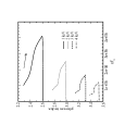
Figure 8.— The trajectory in the photon index $\alpha$ and luminosity plane for a non-expanding model A1. The evolution is clockwise.

Figure 9.— The light curves for expansion cases: exp-C1 (top) exp-A1 (bottom). In the top panel, a non-expanding model A1 is also shown by thin curves for comparison.

Figure 10.— The light curves for expansion cases with exp-C1 ($t_{1}=6\times 10^{5}$ s) and exp-C2 ($t_{1}=8\times 10^{5}$ s). Thick curves are for exp-C1 and thin curves are for exp-C2

Figure 11.— The trajectory in the photon index and luminosity plane for expansion cases: model exp-A1 (thick curves) and exp-C1 (thin curves).

References

- Band & Grindlay (1986) Band, D., & Grindlay, J. E., 1986, ApJ, 311, 595
- Bregman (1990) Bregman, J., 1990, A&ARev, 2, 125
- Celotti, Maraschi, & Treves (1991) Celotti, A., Maraschi, L., & Treves, A., 1991, ApJ, 377, 403
- Canuto & Tsiang (1977) Canuto, V., & Tsiang, E., 1977, ApJ, 213, 27
- Chiaberge & Ghisellini (1999) Chiaberge, M., & Ghisellini, G., 1999, MNRAS, 306, 551
- Christiansen, Scott, & Vestrand (1978) Christiansen, W. A., Scott, J. S., & Vestrand, W. T., 1978, ApJ, 223, 13
- Dermer (1998) Dermer, C. D., 1998, ApJ, 501, L157
- Dermer, Sturner, & Schlickeiser (1997) Dermer, C. D., Sturner, S.J., & Schlickeiser, R., 1997, ApJS, 109, 103
- Georganopoulos & Marscher (1998) Georganopoulos, M., & Marscher, A. P., 1998, ApJ, 506, 11
- Ghisellini & Celotti (2001) Ghisellini, G. & Celotti, A., 2001, astro-ph/0106570
- Ginzburg & Syrovatskii (1965) Ginzberg, V. L., & Syrovatskii, S. I., 1965, ARAA, 3, 297
- Jones & Tobin (1977) Jones, T. W., & Tobin, W, 1977, ApJ, 215, 474
- Königl (1978) Königl, A., 1978, ApJ, 225, 732
- Kirk it et al (1994) Kirk, J. G., Melrose, D. B., Priest, E. R., 1994, Plasma Astrophysics (Berlin: Springer-Verlag)
- Kirk, Rieger & Mastichiadis (1998) Kirk, J. G., Rieger, F. M., & Mastichiadis, A., 1998, A&A, 333, 452
- Kusunose, Takahara, & Li (2000) Kusunose, M., Takahara, F., & Li, H., 2000, ApJ, 536, 299
- Li & Kusunose (2000) Li, H., & Kusunose, M., 2000, ApJ, 536, 729
- Marscher (1980) Marscher, A. P., 1980, ApJ, 239, 296
- Marscher & Gear (1985) Marscher, A. P., & Gear, W. K., 1985, ApJ, 298, 114
- Marshall et al., (2001) Marshall, H. L., et al., 2001, ApJ, 549, L167
- Mastichiadis & Kirk (1997) Mastichiadis, A., & Kirk, J. G., 1997, A&A, 320, 19
- Mathews (1971) Mathews, W. G., 1971, ApJ, 165, 147
- Narayan & Yi (1994) Narayan, R., & Yi, I., 1994, ApJ, 428, L13
- Ozernoy & Sazonov (1968) Ozernoy, L. M., & Sazonov, V. N., 1968, Nature, 219, 467
- Pacholczyk (1970) Pacholczyk, A. G., 1970, Radio Astrophysics (San Francisco: Freeman)
- Rees (1966) Rees, M. J., 1966, Nature, 211, 468
- Rees (1967) Rees, M. J., 1967, MNRAS, 135, 345
- Rees et al (1982) Rees, M. J., Phinney, E. S., Begelman, M. C., & Blandford, R. D., 1982, Nature, 295, 17
- Reeves & Turner (2000) Reeves, J. N., & Turner, T. J, 2000, MNRAS, 316, 234
- Sambruna, Eracleous & Mushotzky, (1999) Sambruna, R., Eracleous, M., & Mushotzky, R. F., 1999, ApJ, 526, 60
- Schlickeiser (1984) Schlickeiser, R., 1984, A&A, 136, 227
- Sedov (1969) Sedov, L., 1969, Similarity and dimensional method in mechanics, (New York: Academic Press Inc.), Chap. IV
- Tagger & Pellat (1999) Tagger, M., & Pellat, R., 1999, A&A, 349, 1003
- Ulrich, Maraschi & Urry (1997) Ulrich, M. -H., Maraschi, L., & Urry, M. C., 1997, ARAA, 35, 445
- Urry & Padovani (1995) Urry, C. M., & Padovani,P.,1995, PASP, 107, 803
- Vitello & Pacini (1977) Vitello, P., & Pacini, F., 1977, ApJ, 215, 756
- Vitello & Pacini (1978) Vitello, P., & Pacini, F., 1978, ApJ, 220, 756
- (38) Vitello, P., & Salvati, M., 1976, Phys. Fluids, 19, 1523
- Wang & Zhou (1995) Wang, J. -M., & Zhou, Y.Y., 1995, ApS&S, 229, 79
- (40) Wang, J. -M., Yuan, Y. -F., Wu, M., & Kusunose, M., 2000, ApJ, 541, L41 (Paper I)
Table 1. The input parameters in the present model