Chemical abundance patterns – fingerprints of nucleosynthesis in the first stars

The interstellar medium of low-metallicity systems undergoing star formation will show chemical abundance inhomogeneities due to supernova events enriching the medium on a local scale. If the star formation time-scale is shorter than the time-scale of mixing of the interstellar matter, the inhomogeneities are reflected in the surface abundances of low-mass stars and thereby detailed information on the nucleosynthesis in the first generations of supernovae is preserved. Characteristic patterns and substructures are therefore expected to be found, apart from the large scatter behaviour, in the distributions of stars when displayed in diagrams relating different element abundance ratios. These patterns emerge from specific variations with progenitor stellar mass of the supernova yields and it is demonstrated that the patterns are insensitive to the initial mass function (IMF) even though the relative density of stars within the patterns may vary. An analytical theory of the formation of patterns is presented and it is shown that from a statistical point of view the abundance ratios can trace the different nucleosynthesis sites even when mixing of the interstellar medium occurs. Using these results, it should be possible to empirically determine supernova yields from the information on relative abundance ratios of a large, homogeneous sample of extremely metal-poor Galactic halo stars.

1 Introduction

During the last decade, the methods for abundance determinations for faint Pop. II stars have reached a stage when accurate abundance ratios can be obtained for great samples of stars with overall metallicities below $1/100$, and even $1/1000$, of the solar. This has made it possible to explore not only abundance trends, e.g. the variation of oxygen or magnesium abundances with decreasing iron abundance, but also the intrinsic scatter in abundance ratios such as Eu/Fe, at a given Fe/H as a function of Fe/H.

An early example of a detailed discussion of the dispersion in abundance ratios was that of Edvardsson et al. (1993) in their study of the chemical evolution of the Galactic disk. These authors found a significant scatter in Fe/H for Disk stars of a given age and a given galactocentric mean distance; however, they did not find any tendency for e.g. Mg/Fe or other $\alpha$-element/iron abundance ratios to scatter at a given overall metallicity, except for the most metal-poor stars. A tendency for these latter stars could be interpreted as the result of a greater star-formation rate (SFR) in the inner Galaxy. In their study of Pop. II dwarfs Nissen at al. (1994) found that the scatter in abundance ratios Mg/Fe, Ca/Fe or Ti/Fe for their sample of Galactic halo stars with $-3.2\leq$[Fe/H] $\leq-1.8$ was less than $0.06$ dex. They also found an upper limit in the scatter in O/Fe of $0.15$ dex. Since the yields of these different elements are different from supernovae (SNe) of different masses, the authors could conclude from the small abundance scatter that the elements observed in the stars must be the results of at least about 20 SN explosions, otherwise statistical fluctuations in abundances should have been present.

The fact that a scatter in abundance ratios for the most metal-poor stars should result from a small number of SNe, with different masses and therefore different yields of heavy elements, was also pointed out by Audouze & Silk (1995). McWilliam et al. (1995) explained the large scatter in s-process element abundances like Ba/Fe and Sr/Fe for [Fe/H]$\leq-2$ in similar terms (see also McWilliam et al. 1996; McWilliam 1998; Ryan et al. 1996).

The abundance scatter for Halo stars has also been modelled. In a stochastic Halo formation model Argast et al. (2000) studied the scatter in relative abundances as resulting from the small number of SNe contributing to the abundances for the most metal-poor stars; these authors found that a great scatter should be expected in several ratios for stars with [Fe/H]$<-3$, representing early evolutionary phases when the interstellar medium (ISM) of the Halo was unmixed and dominated by local inhomogeneities. In the range where [Fe/H] increases from $-3$ to $-2$ there is a gradually diminishing scatter due to the contribution from an increasing number of SNe and more mixing in the ISM, while for still higher metallicities the Halo ISM is well mixed, and homogeneous abundance ratios result. Recent studies, empirical as well as theoretical, of chemical inhomogeneities in the Galactic halo have also included work on r-process elements (notably Eu, as well as Ba, see Ishimaru & Wanajo 1999; Raiteri et al. 1999; Travaglio et al. 2001 and references given there) and Be and B (e.g. Suzuki et al. 1999). In particular, Tsujimoto et al. (2000 and references therein) have developed a stochastic chemical evolution model to study the effects of inhomogeneous r- and s-process element enrichment in the early Galaxy. Some of their relative abundance diagrams show features resembling those to be discussed here.

There are today three identified metal-poor Halo stars with dramatic r-process signatures where CS 22892-052 is the most famous one (Sneden et al. 1996). The identification of such extreme outliers gives important clues to the understanding of the nucleosynthesis in these early SN explosions. However, it is not possible to determine, from the outliers alone, which type of SN (i.e. what progenitor mass) is able to produce such an abundance signature, nor to estimate the relative significance of different SNe with other progenitor masses. In this paper, we shall present an alternative approach to unveil the statistical properties of SNe, taking into account a whole population of extremely metal-poor stars. The effects from a small number of SNe affecting the chemical composition of these stars are explored. We shall demonstrate the probable presence of fine structure patterns in the diagrams where abundance ratios are plotted relative to each other, reflecting the number of SNe contributing and the sometimes strong mass dependence of the yields. In fact, we shall argue that these patterns, if observed, could be used for empirically exploring such properties further. Some preliminary results of our work were published in Karlsson & Gustafsson (2000).

After some general comments and definitions in Sect. 2, we shall present our simulations in Sect. 3. The origin of the patterns is further analysed in Sect. 4, wherein an analytical theory of the distributions of stars in different abundance planes is developed. Observational implications are discussed in Sect. 5 and the conclusions are presented in Sect. 6. In the Appendix, we derive some general expressions describing the statistics of random variables.

2 Chemical enrichment in metal-poor systems

Local chemical inhomogeneities in the interstellar medium, caused by the first generations of SNe in the Galaxy, may or may not be preserved in subsequent generations of stars, depending on how efficient the mixing of the ISM is relative to the rate of star formation. The global mixing can be defined in terms of a mixing efficiency parameter, $\epsilon_{\mathrm{mix}}$, which describes how fast the mixing occurs as measured in, say, solar masses per million years. Hence, $\tau_{\mathrm{mix}}\propto M_{\mathrm{system}}/\epsilon_{\mathrm{mix}}$, where $M_{\mathrm{system}}$ is the total mass of the system. The mixing efficiency parameter can also be used to define a characteristic mixing mass, such that $M_{\mathrm{mix}}=\epsilon_{\mathrm{mix}}\tau_{\mathrm{SF}}$, where $\tau_{\mathrm{SF}}\propto\mathrm{SFR}^{-1}$ is the star formation time-scale.

Thus, if the mixing is efficient enough or/and the star-formation rate is low, the time-scale of global mixing is much shorter than the star formation time-scale, or equivalently, $M_{\mathrm{mix}}$ is comparable to $M_{\mathrm{system}}$. In this case the inhomogeneities are wiped out before subsequent generations of stars are formed and the system will be considered well mixed at any instant of time. The stars will reflect the cumulative build-up of the elements and the whole stellar population has, in this case, a common chemical history meaning that a time-axis can be defined. This, in turn, implies the existence of an age-metallicity relation. On the other hand, if $\tau_{\mathrm{mix}}\gg\tau_{\mathrm{SF}}$, i.e., if $M_{\mathrm{mix}}\ll M_{\mathrm{system}}$ the stars would trace the local fluctuations caused by individual enrichment events and the chemical inhomogeneous state of the system would be resolved and preserved by low-mass (yet unevolved) stars. Such a system can not be considered evolving with time in a unique way since the stars in the system describe different chemical histories. Hence, a single age-metallicity relation does not exist.

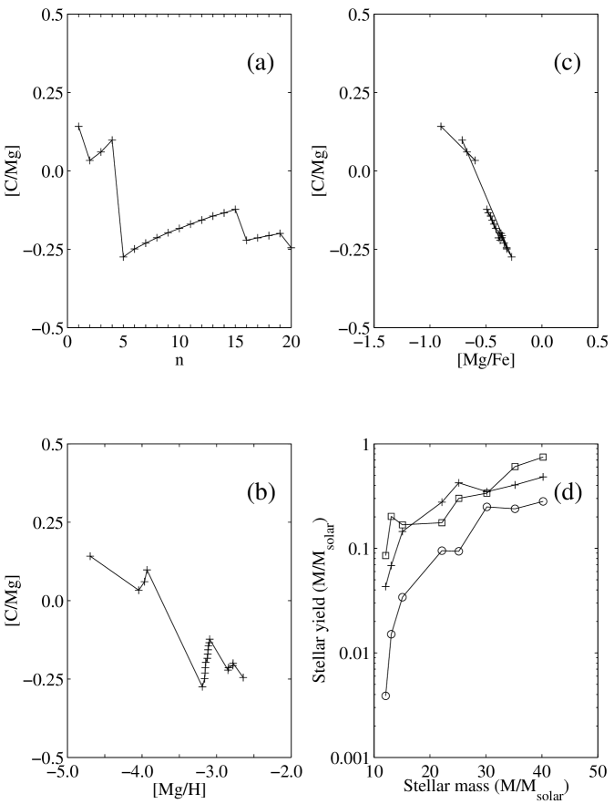
Figure 1: a) A sequential build-up of the C/Mg ratio. The ratio changes when the contribution from another SN is added. The number of SNe is denoted by $n$. b) The chemical track in the [Mg/H]–[C/Mg] plane. The amount of magnesium is mixed with $5\times 10^{5}\leavevmode\nobreak\ \mathcal{M_{\odot}}$ of hydrogen in calculating the Mg/H ratio. c) The chemical track in the [Mg/Fe]–[C/Mg] plane. d) The variation of the stellar yields with SN mass taken from the zero-metallicity models of Woosley & Weaver (1995). The pluses ($+$) denote the carbon yield, the open circles ($\circ$) denote the magnesium yield and the squares ($\Box$) denote the iron yield. Note the downturn in the carbon yield at $\sim 25\leavevmode\nobreak\ \mathcal{M_{\odot}}$. At the same mass, the Mg-yield increases. This is reflected by the jumps in the chemical tracks

Let us discuss in more detail how the chemical enrichment of the ISM can be reflected in the stellar population. Suppose that we have a system which initially consists of primordial gas (i.e. $Z_{\mathrm{init}}=0$). Assume that the instantaneous recycling approximation is valid and that the whole system is well mixed at all times, i.e. $\tau_{\mathrm{mix}}\ll\tau_{\mathrm{SF}}$. Any massive star that explodes immediately pollutes the whole system and the chemical composition of the ISM is changed accordingly. Let us call a chain of such enrichment events a chemical series. Note that the progenitor masses of the SNe do not follow a decreasing sequence, they are randomly distributed. A finite part of a series, say, up to $i$ SNe, shall be referred to as a chemical sequence which describes the chemical state of the system at the time when $i$ SNe have exploded. A star formed out of this gas is a realization of the chemical sequence. Now, if low-mass stars are continuously formed over time the complete enrichment history of the ISM is mapped. The chemical evolution of the system is then followed by displaying the stars in different abundance diagrams. Such time-lines shall be called chemical tracks and are realizations of the chemical series up to a certain number, $n$, of SNe. Since the ISM is homogeneous there exists only one chemical series in the system. This is illustrated in Fig. 1 by the sequential build-up of the C/Mg ratio. Two chemical tracks related to the C/Mg ratio are also shown (Fig. 1b, 1c). The distinct jumps in Figs. 1a and 1b reflect the enrichment of the ISM by a massive SN. The yields as functions of progenitor mass are shown in Fig. 1d.

Systems like the one discussed above show unique chemical tracks for each pair of elements (or element ratios). This is clear since the chemical state of such a system at any time is described by a single chemical series. Suppose now that $M_{\mathrm{mix}}\ll M_{\mathrm{system}}$, i.e. our system consists of a number of separate subsystems, or star-forming regions. As above, the instantaneous recycling approximation is valid for each region but the different subsystems evolve differently, and their chemical states are described by different chemical series. A population of stars, randomly picked from different star-forming regions would, then, describe the chemical evolution of several systems, leading to a large star-to-star scatter in the observed abundances. However, due to the many different enrichment histories of these stars, substantially more information on the elemental production sites (described as stellar yields) is preserved and we shall see that the distribution of stars in the abundance diagrams show structures and patterns created by specific variations in the SN yields with progenitor mass which can provide detailed clues to the production of elements in the early Galaxy.

3 Simulations of the chemical patterns

The existence of a large scatter in abundance ratios for the Galactic halo stars with [Fe/H]$<-2.5$ suggests the second scenario (i.e. $\tau_{\mathrm{mix}}\gg\tau_{\mathrm{SF}}$) discussed in Sect. 2. Below, we shall simulate the chemical enrichment of such a metal-poor system. In all our simulations particular data on SN yields will be applied. These data are rather uncertain, not the least as regards the variations of the yields with stellar mass, which also makes our actual predicted abundance patterns uncertain. Our point here is, however, not to make exact predictions but to illustrate the general effects of mass-dependent yields.

3.1 General assumptions

The gaseous medium of the system (i.e. the Galactic halo) is assumed to be initially primordial, i.e., $Z_{\mathrm{init}}=0$. The characteristic mixing mass is assumed to be much smaller than the total mass of the system, such that $M_{\mathrm{mix}}\ll M_{\mathrm{system}}$. This is realized by assuming $M_{\mathrm{mix}}$ to be of the same order of magnitude as the localized star-forming regions of, say, $\sim 10^{6}\leavevmode\nobreak\ \mathcal{M_{\odot}}$ each. From the number of Halo horizontal branch stars, Binney & Merrifield (1998) estimate the present day mass of the stellar component of the Halo to $\sim 10^{8}\leavevmode\nobreak\ \mathcal{M_{\odot}}$, which implies that the total mass of the Halo was, at least, on the order of $M_{\mathrm{system}}=10^{9}\leavevmode\nobreak\ \mathcal{M_{\odot}}$ in the early epochs. Thus, $M_{\mathrm{mix}}/M_{\mathrm{system}}\sim 10^{-3}$.

We shall distinguish between abundances measured relative to hydrogen, and abundance ratios between different, more heavy elements. To trace individual SNe or groups of SNe using a ratio of some element $A$ relative to hydrogen (an $A$/H ratio), requires knowledge about the mixing of the star-forming region after the SNe ejection. Ratios between heavier elements, both produced in a SN, are less sensitive to the mixing. This is due to the fact that an $A$/H ratio, in the first-order expectation, essentially depends on the mean distance from the contributing SNe while ratios between different, heavier elements do not. In our models we first schematically assume that the newly synthesized elements mix with a constant hydrogen mass, i.e. all star-forming regions are supposed to have equal mass. Furthermore, the mixing with the cloud material is assumed to be instantaneous and complete. Subsequently, low-mass star formation occurs within each cloud. This implies that the time-scale of mixing within the region is shorter than the formation time-scale for individual stars which in turn is shorter than the epoch of the star formation activity in the region and the life-time of the region itself.

Recurrent SN explosions may disrupt the regions before local mixing and subsequent star-formation occurs. If this happens inter-cloud mixing has to be taken into account. This will naturally affect abundances relative to hydrogen in the ISM. However, abundance ratios between more heavy elements are, at least statistically, almost unaffected by such a mixing.

Subsequently, we shall discuss two types of abundance-ratio diagrams (in the general case denoted ”$A/$ diagrams” below). Some diagrams will relate the abundances of two heavier elements to hydrogen, such as [C/Mg] vs. [Mg/H]; these are denoted ”$A/$H diagrams”. These diagrams will be affected by the not very well-known degree of mixing of SN remnants with other, less processed, material in the different star-forming regions. Therefore, we shall primarily discuss diagrams displaying the relative abundances between three heavier elements, e.g. [C/Mg] vs. [Mg/Fe], diagrams that are much less sensitive to the mixing uncertainties. This type of diagrams will be denoted ”$A/A$ diagrams” below.

The ejected material from each individual SN is assumed to be well mixed prior to subsequent star formation, such that any stars formed out of this material will all have the same abundances. Both observations (see Travaglio et al. 1999) and hydrodynamical simulations (e.g. Kifonidis et al. 2000) of core collapse supernovae show evidence for substantial mixing of elements shortly after the core bounce (however, see also Hughes et al. 2000; Douvion et al. 1999 where they discuss heterogeneous mixing in the Cas A supernova remnant). The simulations also indicate that the interaction between the processed material and the outer layer of hydrogen (i.e in SNe type II) causes a complete homogenization of the ejected material. This process does not work for stars without a massive hydrogen envelope (i.e. SNe Ib/Ic) for which the mixing might be less pronounced (Kifonidis, private communication).

In our investigation we assume that the stellar yields are one-dimensional functions of progenitor mass of the SN. For convenience, we also assume that stars less massive than $10\leavevmode\nobreak\ \mathcal{M_{\odot}}$ do not produce heavy elements within the time-scales considered here and that the prompt enrichment of the primordial ISM by a population of very massive stars ($>100\leavevmode\nobreak\ \mathcal{M_{\odot}}$) suggested by, e.g., Wasserburg & Qian (2000) did not occur. Recent yield calculations by Umeda et al. (2000) show a moderate metallicity dependence in the lowest metallicity regime for the secondary elements, notably ¹⁴N, ²³Na and ²⁷Al. However, primary elements such as ¹²C, ¹⁶O and ²⁴Mg are almost independent on metallicity. A high dependence enters first after the amount of metals initially present is sufficient to cause extensive mass-loss through radiation-driven winds (Maeder 1992; Portinari et al. 1998). The chemical yields may also be altered by stellar rotation (Heger & Langer 2000). It is straight forward to incorporate rotational dependent yields in the simulations, as well as in the analytical theory presented below (Sect. 4.2). The situation is different for metallicity dependent yields since the metal content in every star is coupled to the history of chemical enrichment. We shall neither consider metallicity- nor rotational dependent yields in the present study.

For the general discussion we shall assume that the amount of any heavy element ejected by a SN of a given progenitor mass is constant from one stellar generation to the next. The ejecta of an element $A$, $e_{A}(m,Z)$, can be written as

$$e_{A}(m,Z)=(m-m_{r})\times Z_{A}^{\mathrm{init}}(t-\tau_{m})+p_{A}(m),$$ (1)

where $m$ is the progenitor mass of the star, $m_{r}$ is the remnant mass, $Z_{A}^{\mathrm{init}}(t-\tau_{m})$ is the initial mass fraction of the element at the time of formation of the star, $\tau_{m}$ is the life-time of stars with mass $m$ and $p_{A}(m)$ is the stellar yield, the mass of element $A$ produced or destroyed in the star. Hence, the total ejected mass is a sum of the initially present amount of $A$ and the newly synthesized amount. For low metallicities the first term on the RHS in Eq. (1) becomes negligible and, thus, the ejected matter is completely dominated by the stellar yield.

We assume the sampled Halo stars to be statistically independent. Thus, we assume that all chemical sequences (i.e. stars) are picked randomly from an infinite number of chemical series. This assumption means physically that the stars that originate from star formation regions where, say, three SNe have exploded sample different such regions, and that stars coming from regions where four SNe have exploded sample still other and different regions. This assumption is further discussed in Sect. 3.4.4 and there found to be reasonable.

3.2 Model I

To simulate the distribution of abundances in Halo stars we adopt the simple picture that star formation and heavy element enrichment of the ISM are confined within star-forming regions of about a Jeans mass each, i.e. a hydrogen mass of $M_{\mathrm{H}}=5\times 10^{5}\leavevmode\nobreak\ \mathcal{M_{\odot}}$. This particular value is chosen ad hoc. Another hydrogen mass would simply introduce a shift in the abundances relative to hydrogen. We place a number of high-mass stars with randomly distributed masses (according to the Salpeter IMF if nothing else is stated) between $10$ and $100\leavevmode\nobreak\ \mathcal{M_{\odot}}$ in the hydrogen clouds and let them explode as core collapse SNe. The total number of SNe exploding in each cloud vary in a range from one to a large number (i.e. up to $\sim 20$). The SNe produce heavy elements according to theoretically calculated stellar yields. We shall use the yields by Woosley & Weaver (1995) calculated from their metal-free models (Z models) and by Nomoto et al. (1997). Hereafter, these works will be referred to as WW95 and Netal97, respectively. All yields are extrapolated by a constant to the ends of the mass interval. The yields by WW95 are modified according to the possible decay channels of the unstable isotopes. The high-mass stars explode directly and their ejecta are instantaneously mixed with the cloud material. Hence, these regions are chemically different according to the number and masses of SNe that have formed and enriched the regions. Subsequently, low-mass stars are formed out of the enriched gas. Effectively, this means that we sum up the heavy element contribution from every SN within each cloud. The abundance of any element $A$ relative to hydrogen (by number) is then calculated and taken as the surface abundance of a low-mass star formed in the cloud.

We assume the total number of low-mass stars formed in each cloud to be constant. This implies that there is an equal probability to pick a star tracing one chemical series as it is to pick a star tracing another series, and since the number of star-forming regions is assumed to be large (i.e. the stars are statistically independent) we are allowed to select the stars from different regions. The total number of Halo stars ($N$) in a simulated sample is then governed by

$$N=\sum\limits_{i=1}^{n}W_{i},$$ (2)

where $W_{i}$ is the number of clouds in which $i$ SNe explode and $n$ is the maximum number of SNe that is allowed to explode and enrich a single cloud. In a typical simulation we assume $W_{i}$ to be constant, e.g. $W_{i}=W=25$ for all $i$, thus the total number of stars is $N=n\times W$. By displaying various abundance ratios for low-mass stars in different $A/$ diagrams we are then able to follow the early chemical enrichment phase of an initially metal-free system.

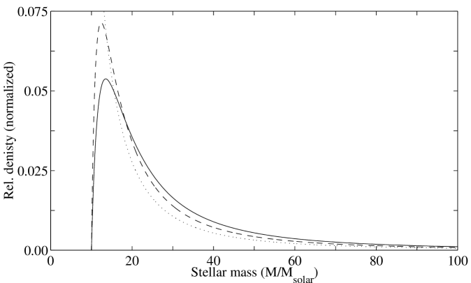
Figure 2: Different mass distribution functions as described by Eq. (4). The full line denotes the relative number density of exploded stars at $t=28.7$ Myrs (corresponding to the life-time of a $10\leavevmode\nobreak\ \mathcal{M_{\odot}}$ star) for a constant SFR. The dashed line denotes the relative number density for an exponential SFR with $t_{\mathrm{SF}}=10$ Myrs. The dotted line is the Salpeter IMF

3.3 Model II

We have alternatively modified our simple chemical enrichment model by introducing continuous star formation in the regions. This mainly affects two parameters, the mass distribution function (which is, in Model I, equal to the IMF) and the lower mass limit of this distribution.

In Model I, the high-mass stars are formed in an initial burst. By allowing the stars (both high- and low-mass stars) to form continuously over a certain period of time we can account for a mass distribution function that changes with time as stars with different masses have different life-times. We shall adopt an exponential star formation rate ($\psi$) such that

$$\psi(t)=\psi_{0}e^{-t/t_{\mathrm{SF}}},$$ (3)

where $t_{\mathrm{SF}}$ is a characteristic time of the star formation. This time is set to the same value in all clouds. Furthermore, suppose that the IMF is a power law of the form $\phi(m)=\phi_{0}m^{-\alpha}$ and introduce $\tau_{m}$, the life-time of a star with mass $m$. The expression for the time-dependent mass distribution function (see Eq. (7.4) in Pagel 1997) describes the distribution of stars over $m$ at a certain $t$. However, we are more interested in the stars that have enriched the cloud at time $t$. The corresponding mass distribution of exploded stars, (see Fig. 2) is governed by

$$f(m,t)=\left\{\begin{array}[]{ll}0,&\tau_{m}>t\\ f_{0}m^{-\alpha}(1-e^{-(t-\tau_{m})/t_{\mathrm{SF}}}),&\tau_{m}\leq t,\end{array}\right.$$ (4)

where $f_{0}=\phi_{0}\psi_{0}t_{\mathrm{SF}}$. The stellar life-times are adopted from the lowest metallicity models of Portinari et al. (1998). Note that in Model I, the function $f(m,t)$ was equal to the IMF since all the high-mass stars were allowed to explode before the formation of the low-mass stars.

The star formation period is assumed to be $\sim 30\leavevmode\nobreak\ \mathrm{Myrs}$ in each cloud. This is only slightly longer than the estimate by Shull & Saken (1995), for OB associations. A lower life-time of the clouds would hinder the formation of stars that could be enriched in elements produced by the least massive SNe, as our models do not take into account global mixing and a second generation of star-forming regions.

Except for the continuous star formation rate Model II is based on the same assumptions as Model I. We adopted a constant star-formation rate in each cloud, which corresponds to a long characteristic time, $t_{\mathrm{SF}}$ (see Fig. 2), leading to a mass distribution of SN progenitors that is significantly different from the IMF. The slope of the IMF was set to $\alpha=2.35$. Furthermore, a read-off time ($t_{\mathrm{read-off}}$), distributed according to the SFR, was generated in each cloud which determined the actual number of polluting SNe, $i$, via an integration of the SFR (up to $t_{\mathrm{read-off}}$) normalized to the total number of high-mass stars in the cloud. The total number of high-mass stars formed in each cloud was randomly generated according to a Gaussian distribution centred at $n=10$ and with $\sigma=20$ (for $n<0$ the probability is zero). Thus, the number of stars that have been enriched by $i$ SNe ($W_{i}$) is not a priori known but is determined after the simulation stops. As mentioned above, this read-off time also sets the lower cut-off of the distribution function of the exploded high-mass stars as no star with a longer life-time than $t_{\mathrm{read-off}}$ has been able to enrich the cloud.

3.4 Results

We should emphasize that a realistic modelling of the early chemical enrichment requires a more physical treatment of the mixing than adopted here. The abundances relative to hydrogen are particularly sensitive. The situation is quite different for abundance ratios, however. They are independent of variations in the mixing mass. They are also insensitive to global, inter-cloud mixing, infall and subsequent generations of star-forming regions (see the discussion in Sect. 4.3). Therefore, we shall, based on this distinction, separately discuss the two corresponding types of $A/$ diagrams.

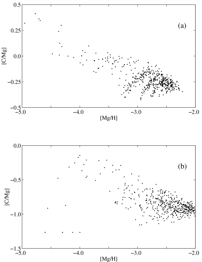
Figure 3: a) A scatter plot of simulated stars in the [Mg/H]–[C/Mg] plane (Model I). The diagram shows $500$ low-mass stars enriched by $1-20$ SNe ($W_{i}=25$). The yields are taken from WW95 and the masses of the SNe, ranging from $10\leavevmode\nobreak\ \mathcal{M}_{\odot}$ to $100\leavevmode\nobreak\ \mathcal{M}_{\odot}$, are distributed according to a Salpeter IMF. b) A scatter plot of stars in the same plane as above, using yields from Netal97. It is seen that the existence of clear patterns in these $A/$H diagrams are dependent on the details of the predicted SN yields

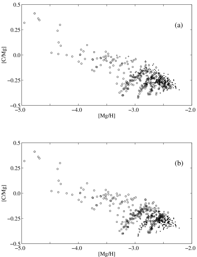
Figure 4: a) Same as Fig. 3a except that the stars are coded. Circles ($\circ$) denote stars enriched by $1-4$ SNe, squares ($\Box$) are enriched by $5-8$ SNe, pluses ($+$) by $9-13$ SNe, diamonds ($\Diamond$) by $14-17$ and dots ($\cdot$) are enriched by more than 17 SNe. b) As above but with a different coding. Circles ($\circ$) denote stars which have not been enriched by any SN with a mass above $27.5\leavevmode\nobreak\ \mathcal{M}_{\odot}$, squares ($\Box$) are enriched by one SN above $27.5\leavevmode\nobreak\ \mathcal{M}_{\odot}$, pluses ($+$) have been enriched by two such SNe, diamonds ($\Diamond$) by three and dots ($\cdot$) by four or more SNe above $27.5\leavevmode\nobreak\ \mathcal{M}_{\odot}$. The patterns displayed reflect the number of high mass SNe that have enriched the ISM before the sample star was formed

3.4.1 $A/$H diagrams

Let us first discuss some properties of the $A/$H diagrams before we turn to the $A/A$ diagrams. We see from Fig. 3 that the appearance of the stars in the diagrams depends naturally on the produced amount of carbon and magnesium in the massive stars. However, the shape of the stellar yield functions are responsible for possible trends and/or the groupings of stars into different substructures and patterns. These structures appear as a result of the various enrichment histories of the low-mass stars (cf. Fig. 1 and the discussion in Sect. 2). Even though we generally do not expect patterns to appear in $A/$H diagrams displaying real observations the overall distribution of stars, such as large-scale trends, can still hold important information. If patterns would really be observed in $A/$H diagrams this would put strong constraints on the star formation and mixing processes in the early Galaxy. There are three effects that are directly observed in the diagrams in Fig. 3 and Fig. 4.

Firstly, the star-to-star scatter seems to decrease with increasing metallicity (represented by [Mg/H]). This is best seen in Fig. 3b and is due to the fact that stars enriched by a single SN have the lowest metallicities and the largest variations in the C/Mg ratio. When more and more SNe contribute to the metal content in the low-mass stars the metallicity increases and the variation in the ratio is averaged out. Note also that stars with a specific metallicity may have been enriched by quite a different number of SNe. For example, at [Mg/H]$\sim-3$ the stars with lowest C/Mg ratio have been enriched by perhaps a couple of SNe while the ones with the highest ratio have been enriched by up to $17$ SNe (see Fig. 4a).

Secondly, in Fig. 3a we see another effect. Instead of a decreasing scatter with metallicity the scatter is asymmetric, mimicking a trend. The C/Mg ratio seems to decrease with increasing Mg/H. This is not a normal evolutionary effect caused by time or metallicity (such as the decrease of [Mg/Fe] with [Fe/H] for [Fe/H]$>-1$ induced by the onset of thermonuclear supernovae (SNe type Ia) or the increase of [C/O] with [O/H] which could be explained by a metallicity dependent carbon yield as proposed by e.g. Gustafsson et al. 1999; Henry et al. 2000) but rather a SN mass (i.e. number) effect. This is accomplished by SNe producing a high C/Mg ratio at the same time produce a small amount of magnesium while SNe producing a low C/Mg ratio also produce much Mg. So, for an extremely metal-poor system an observed trend like this one does not necessarily imply chemical evolution in the normal sense (see also Tsujimoto & Shigeyama 1998).

Thirdly, the stars in Fig. 3a tend to group together in substructures. It is understood from Fig. 4b that these patterns are caused by a specific variation with progenitor mass in the carbon yield. Roughly, one can say that these patterns are formed by a pronounced decrease in the yield around $27.5\leavevmode\nobreak\ \mathcal{M}_{\odot}$. We shall discuss these issues in more detail in Sect. 4. As we have mentioned, the substructures in Fig. 3a are sensitive to variations in the mixing mass. As long as all star-forming regions have equal mass these substructures survive. This is unlikely, however. Nakasato & Shigeyama (2000) discuss metal enrichment of the primordial ISM by individual SNe and find that the Mg/H ratio in various filaments may differ by $\sim 1.0$ dex, implying a large abundance scatter in the second generation of stars. Thus, a smearing effect most probably occurs in the horizontal direction in the diagrams of Figs. 3 and 4. The fact that we see patterns in the $A/$H diagrams is because we have not included this type of mixing in the models.

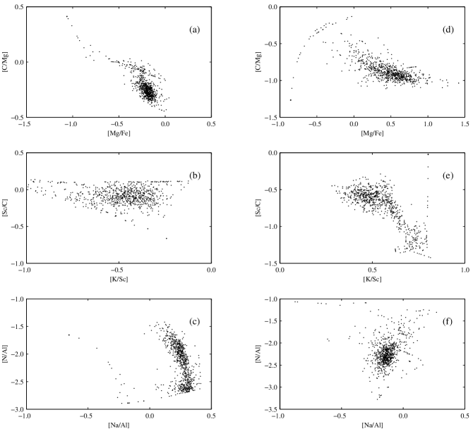
Figure 5: Scatter plots of stars as they may appear in different $A/A$ diagrams. a-c) Simulated stars (Model I) enriched by 1 – 20 SNe using yields from WW95. d-f) The corresponding $A/A$ diagrams produced with yields taken from Netal97. Note that for a particular abundance plane the difference (apart from the loci) between the distributions is large which arises from differences in the yields

3.4.2 $A/A$ diagrams

Using Model I, it is possible to generate pure abundance ratios which can be displayed in $A/A$ diagrams such as those in Fig. 5. The patterns that are formed in these kinds of diagrams, opposed to the ones in the $A/$H diagrams, are insensitive to intrinsic uncertainties such as mixing. They also show larger variations in their shapes. For observational uncertainties of $\simeq 0.1$ dex in the Mg/H and C/Mg ratios the two scatter plots in Fig. 3a and b would appear quite similar apart from the different loci. However, for the same uncertainties in the C/Mg and Mg/Fe ratios the difference between the chemical patterns in Figs. 5a and 5d will survive. It is obvious that the stellar yields play a crucial role in the formation of these patterns. The other pairs in Fig. 5 show even larger differences due to larger disagreements in the two sets of yields (i.e. WW95 and Netal97).

Model I and Model II generate $A/A$ diagrams showing strong similarities. By comparing Fig. 6a and Fig. 5e we see that the stars are arranged in the same manner, apart from minor differences in the distribution within the formed pattern. This is a result of the discrete enrichment as the abundance ratios are not considered to be weighted with an IMF or some other mass distribution function. A set of yields generates a unique pattern while the mass frequency of SNe determines how the pattern will be populated by low-mass stars. In Sect. 4.2, we shall derive a mathematical expression for this statement. Note that the concentration of stars in the upper part of the distribution in Fig. 6a results from a higher density of individual SNe producing these abundance ratios (cf. the red curve in Fig. 8e).

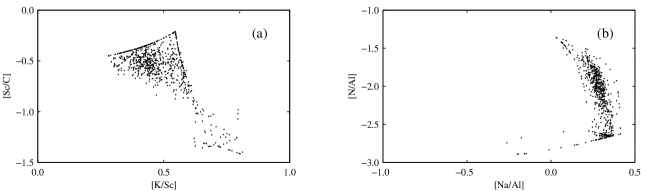
Figure 6: a) The distribution of stars in the [K/Sc]–[Sc/C] plane (cf. Fig. 5e) as predicted by Model II. Due to the evolutionary effect the highly enriched stars do not converge to a point in the diagram even though they have been enriched by many SNe. This effect is not easily detected, however. b) Same as Fig. 5c as predicted by Model II

In Model II, the relaxation of the instantaneous recycling approximation within the star-forming regions introduces an evolutionary effect which has no counterpart in Model I. This effect should appear as a finite, non-vanishing dispersion in the different abundance ratios when the number of polluting SNe becomes large. The dispersion survives because stars that are formed early could only have been enriched by the most massive stars while stars that are formed late (i.e. $\sim 30\leavevmode\nobreak\ \mathrm{Myrs}$) could have been be enriched by SNe of any mass. However, the effect can not easily be detected in the the patterns in Fig. 6. In fact, this is as expected since we only use a maximum number of $20$ SNe in our simulations, which implies that the statistical fluctuations in the abundance ratios is still comparable to this dispersion. Eventually, the interaction between different clouds mixes the gas and the chemical abundance scatter in the subsequent generation of stars is decreased.

3.4.3 Possible sources of contamination

In our models we have assumed that the only stars that enrich a star-forming region with heavy elements have masses $\geq 10\leavevmode\nobreak\ \mathcal{M_{\odot}}$, excluding the very massive stars ($>100\leavevmode\nobreak\ \mathcal{M_{\odot}}$). This is consistent with the life-time of the star-forming regions adopted, i.e. $30$ Myrs. One could ask whether also intermediate-mass stars could be able to enrich a cloud. This would require that that either the life-time of the region is longer than assumed, or that the intermediate-mass stars were formed in epochs before the formation of the star-forming region. In the latter case it is reasonable to assume that the region has also been polluted by more short-lived, high-mass SNe. That is, none of the Halo stars would be enriched by a single, intermediate-mass star. The chemical patterns would be blurred but probably not very significantly.

The patterns could also possibly be affected by a population of very massive stars, preceding the onset of normal core collapse SNe. Similarly to the intermediate-mass stars, the very massive stars would pollute the star-forming regions with unknown amounts of elements, not accounted for in the models.

Another, related source to noise affecting the patterns is the possible existence of stars sampling the nucleosynthetic signature of thermonuclear supernovae, like SNe type Ia. They are a different type of objects, not parametrized by the progenitor mass, and they will introduce a pattern in the $A/$ diagrams which is different from that of the core collapse supernovae. Progenitors of early thermonuclear SNe are thought to be close binary systems in which a white dwarf accrets matter from a subgiant star with a mass of $2$-$3.5\leavevmode\nobreak\ \mathcal{M_{\odot}}$ (Branch 1998). The time delay between the onset of star formation and the formation of these thermonuclear SNe are at least on the order of $0.1$ Gyrs. Thus, the core collapse SN patterns in the $A/$ diagrams may not be severely contaminated by these objects.

As mentioned in Sect. 3.1 we do not consider metallicity dependent yields in our models. Such yields may also produce a smearing of the chemical patterns. The smearing is small for primary elements but could be as large as $0.5$ dex for secondary elements, e.g., for the ratio ${}^{14}\mathrm{N}/^{24}\mathrm{Mg}$ (Umeda et al. 2000).

In general, it would not be easy to recognize and remove stars enriched by these extra, hypothetical sources, except perhaps for stars with abundance patterns indicative of a pure thermonuclear SN contribution. However, we have presently no strong reasons to believe that any of these sources have a significant effect on the $A/$ diagrams.

3.4.4 The effects of statistical dependence

Since the number of star-forming regions in reality is not infinite there is a certain probability that two, randomly picked Halo stars may have formed in the same cloud, or equivalently, the observed sample of stars may not be completely statistically independent. If we randomly pick a number of stars which have been formed in a certain number of star-forming regions, how many of these regions are then represented by these stars? If the total mass of the Halo at the early epochs was ten times the mass of the stellar component today, which is $\sim 10^{8}\leavevmode\nobreak\ \mathcal{M_{\odot}}$ (Binney & Merrifield 1998), and all the gas was confined in star-forming regions of $10^{6}\leavevmode\nobreak\ \mathcal{M_{\odot}}$, there were approximately $1000$ different regions. Assume that every region formed an equal amount of stars. From available statistics (Christlieb & Beers 2000 and references therein) we estimate that there are approximately $50\leavevmode\nobreak\ 000$ extremely metal-poor Halo stars with a $B$ magnitude $\leq 17$. Now, suppose that we randomly select a subsample of $100$ stars. How many different star-forming regions (sampling different chemical series) are then represented by the sample? Given the much larger number of available Halo stars, we estimate that approximately $95\%$ of the selected stars would sample different regions. On the other hand, if no more than $100$ star-forming regions existed in the early Galaxy, about $63$% of the stars would still be statistically independent.

We performed a small test to investigate the necessity of the assumption of statistical independence. We generated two samples containing $1000$ stars each. The stars in the first sample were selected from individual chemical series where no star was enriched by more than $25$ SNe. These stars are statistically independent. The second sample consisted of $40$ chemical tracks, i.e., all stars enriched by $1-25$ SNe were selected from $40$ different chemical series. Stars belonging to a chemical track have a common chemical history and are statistically dependent. The difference between the two corresponding $A/$ diagrams was found to be relatively small and the characteristic pattern displayed by the first sample was well reproduced by the second one. Since only some tens independent chemical series contain enough information to form reliable patterns (remember that $100$ randomly selected Halo stars would sample maybe twice as many series), we conclude that the assumption of statistical independence is not vital for our conclusions.

4 The origin of the chemical patterns

In this section we shall discuss the origin of the chemical patterns found in the simulations above. We start with an approximate approach to elucidate the source of the patterns, and also give some further insight into the reason for the variety of patterns, demonstrated in Fig. 5 before we turn to the analytical theory.

4.1 Approximate approaches to pattern formation

Let us, to be explicit, assume that the yields for three elements, $A$, $B$ and $C$, vary with mass such that, i.e, element $A$ is predominantly produced by SNe in a certain progenitor mass range, $m_{A^{\prime}}$ to $m_{A^{\prime\prime}}$, with yield $p_{A^{\prime}}$, and for the rest of the mass interval the yield is assumed to be much lower and constant, $p_{A^{\prime\prime}}$. Similarly, the element $B$ is assumed to be produced by stars in the disjoint mass range $m_{B^{\prime}}$ to $m_{B^{\prime\prime}}$, with yield $p_{B^{\prime}}$, while the stars outside the interval produce the element $B$ with the much lower yield $p_{B^{\prime\prime}}$. The element $C$ is assumed to be produced with a mass-independent yield $p_{C}$. Denote the number of SNe within the progenitor mass interval ($m_{A^{\prime}}$,$m_{A^{\prime\prime}}$) by $n_{1}$, and correspondingly $n_{2}$ for the mass interval ($m_{B^{\prime}}$,$m_{B^{\prime\prime}}$). The total number of SNe is denoted $n_{3}$.

Figure 7: Generic $A/A$ diagram generated from artificial yields. two pronounced peaks in the $A$ and $B$ yields produce the characteristic ”L”-shape with a cluster of stars round the centre of gravity

With these assumptions it is easy to derive the main properties of the distribution of stars in the [$A$/$C$]–[$B$/$C$] plane (Fig. 7). We find the total yields of element $A$, $B$ and $C$ to be, respectively

$$P_{A}=n_{1}p_{A^{\prime}}+(n_{3}-n_{1})p_{A^{\prime\prime}}$$ (5)

$$P_{B}=n_{2}p_{B^{\prime}}+(n_{3}-n_{2})p_{B^{\prime\prime}}$$ (6)

$$P_{C}=n_{3}p_{C}.$$ (7)

The extreme point in the lower left corner of the ”L”-shaped distribution in Fig. 7 will have the locus $\{\log(p_{A^{\prime\prime}}/p_{C}),\log(p_{B^{\prime\prime}}/p_{C})\}$, and the end points of the ”L” will be at $\{\log(p_{A^{\prime}}/p_{C}),\log(p_{B^{\prime\prime}}/p_{C})\}$ and $\{\log(p_{A^{\prime\prime}}/p_{C}),\log(p_{B^{\prime}}/p_{C})\}$, respectively. These points correspond to cases with no SNe in the mass intervals ($m_{A^{\prime}}$,$m_{A^{\prime\prime}}$) and ($m_{B^{\prime}}$,$m_{B^{\prime\prime}}$), ($m_{B^{\prime}}$,$m_{B^{\prime\prime}}$), and ($m_{A^{\prime}}$,$m_{A^{\prime\prime}}$). Obviously, if these points can be observed, the yields can all be determined.

If one further assumes that $n_{1}p_{A^{\prime}}\gg(n_{3}-n_{1})p_{A^{\prime\prime}}$ and that $n_{2}p_{B^{\prime}}\gg(n_{3}-n_{2})p_{B^{\prime\prime}}$ one finds the centre of gravity of the points in the $A/A$ diagram to be at $\{\log(p_{A^{\prime}}/p_{C})-\log(n_{3}/n_{1}),\log(p_{B^{\prime}}/p_{C})-\log(n_{3}/n_{2})\}$. Thus, with the yields known observation of this point gives the ratios

$$\frac{n_{3}}{n_{1}}=\frac{\int_{10}^{100}\phi(m)dm}{\int_{m_{A^{\prime}}}^{m_{A^{\prime\prime}}}\phi(m)dm}$$ (8)

and

$$\frac{n_{3}}{n_{2}}=\frac{\int_{10}^{100}\phi(m)dm}{\int_{m_{B^{\prime}}}^{m_{B^{\prime\prime}}}\phi(m)dm}.$$ (9)

For the standard deviation in [$A$/$C$] and [$B$/$C$] one finds with the assumptions above $\sigma_{\mathrm{[}A/C\mathrm{]}}\sim 0.4/\sqrt{n_{1}}$ and similarly $\sigma_{\mathrm{[}B/C\mathrm{]}}\sim 0.4/\sqrt{n_{2}}$.

These estimates are, however, very dependent on the assumed yields – yields varying with stellar mass in more complex ways will contribute to the standard deviations, and thus make determination of $n_{1}$ and $n_{2}$ in this way unrealistic.

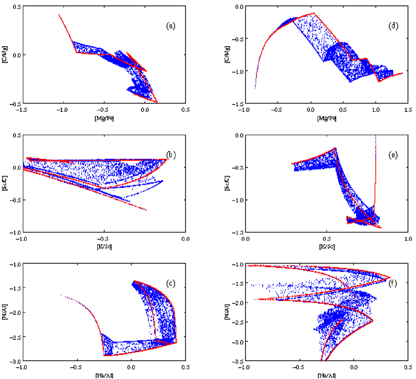
Figure 8: As Fig. 5 but for one and two polluting SNe only. The red dots denote stars enriched by one SN. These stars are located along one-dimensional curves in the abundance planes. The blue dots denote stars enriched by two SNe. Already two polluting SNe account for most of the structures present in the diagrams in Fig. 5

The two legs of the ”L”-shaped distribution in Fig. 7 result from the SNe with no strong contribution of elements $A$ and $B$, respectively. The sparsely populated narrow sequences in Figs. 5 and 6 are, however, mainly the result of the pollution of the star-forming region by just one SN. The sequences are delineated by the range of SNe with different progenitor mass. This is illustrated in Fig. 8, where the corresponding distributions for just one SN (red dots), instead of $1-20$ SNe as in Fig. 5, have been plotted. If such narrow sequences could be identified observationally, which would require rich samples of very metal-poor stars and high observational accuracy, one might directly read off the relative yields at different progenitor masses. The values of the latter will, however, remain unknown.

In Fig. 8 we have also plotted the distributions of stars, resulting from cases with two polluting SNe (blue dots). It is clear from this figure, in comparison with Fig 5, that most of the structure of the $A/A$ diagrams is delineated already by models with two SNe. The density distribution in the diagrams of Fig 5, is, however, determined by the IMF as transformed by the mass dependence of the yields.

4.2 An analytical approach

We shall now proceed to a more exact treatment of the formation of the chemical patterns by deriving analytical expressions for the density distribution (i.e. frequency distribution) of stars in the $A/$ diagrams. This distribution is represented by a two-dimensional density function. It is constructed by a sum of density functions, where each of these functions describes the distribution of stars enriched by a certain number of SNe. In order to understand these functions and get a feeling for the parameter dependence we shall begin by discussing one-dimensional density functions describing the distribution of a specific element or a ratio between two elements. The fundamental functions in this context are the ones that describe the distribution of stars enriched by individual SNe. In Appendix A we derive some general expressions for distributions of random variables and we shall frequently refer to those results in this section.

The analytical theory is based on our simple model of chemical enrichment (i.e. Model I). Its only important parameters are the stellar yields and the IMF slope index. The chemical patterns predicted by Model II are very much like the ones from Model I and the main result from Model I is not altered even if some changes in the density distribution of stars occur. The conclusion is that the stellar yields, or rather the variations in the yields with progenitor mass, play the crucial role for the shape of these density functions.

4.2.1 The element distribution from individual supernovae

We start with deriving the fundamental expression for the distribution of stars enriched by individual SNe. In general terms, the relative frequency of stars in an $A/$ diagram is given by the relative frequency of heavy element producing phenomena as a function of the amount of heavy elements produced. In this study, we assume that these elements are produced in SN explosions and that the number density of SNe is basically determined by $\phi$, the IMF. We have seen above that the actual number density is different from that of the IMF if, e.g., we consider continuous star-formation (Model II). However, this has not a big impact on the formation of the patterns.

First, we need some definitions. The mass of a star formed in a star-forming region can be regarded as a random variable (r.v.) $M$, with a distribution function $F_{M}(m)$. The probability density function is then

$$f_{M}(m)\equiv F_{M}^{\prime}(m)\equiv\phi(m)=\phi_{0}m^{-\alpha},$$ (10)

normalized as

$$\int\limits_{m_{\mathrm{min}}}^{m_{\mathrm{max}}}\phi(m)\mathrm{d}m=1.$$ (11)

We say that $M$ is an $\mathrm{IMF}(m_{\mathrm{min}},m_{\mathrm{max}})$-distributed random variable. Normally, the mass density, $m\phi(m)$, is normalized to one but since we are interested in number densities we choose to normalize $\phi(m)$ instead. Furthermore, let the yield be a continuous function of stellar mass, $x=p(m)$, defined on the interval $[m_{\mathrm{min}},m_{\mathrm{max}}]$, i.e. $[10,100]$.

Now, as stellar masses are randomly distributed (according to this IMF) the amount of an element $A$, produced in a star of mass $m$, will also be randomly distributed ($A$ stands for an arbitrary heavy element which is a product of stellar nucleosynthesis). However, the distribution of the r.v. $X_{(A)}=p_{(A)}(M)$ is different from that of $M$. The probability of $X_{(A)}$ to be less or equal to $x$ is given by the distribution function $F_{(A)}(x)$, and according to Eq. (25)

$$F_{(A)}(x)=F_{M}(p_{(A)}^{-1}(x)),$$ (12)

assuming that $p_{(A)}(m)$ increases monotonically. For monotonically decreasing functions we will have that $F_{(A)}(x)=1-F_{M}(p_{(A)}^{-1}(x))$. We shall write the element in the subscript within parentheses to distinguish these functions from the final expression which is written without parentheses.

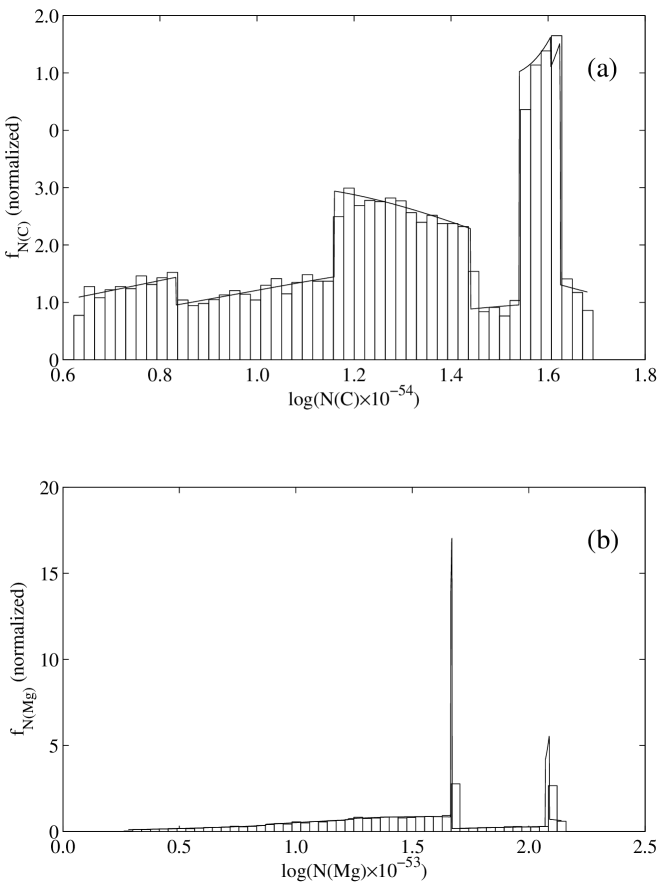
Figure 9: a) The density function of carbon from individual SNe with the yield ($Z=0$ models) taken from WW95 (see Fig. 1d). The Salpeter IMF is used. The histograms are binned data from numerical simulations of $20\leavevmode\nobreak\ 000$ clouds with a single SN explosion in each cloud (Model I) while the full line is the analytical function calculated from Eq. (13) and transformed according to Eq. (40). b) The corresponding density function for the element magnesium

As our aim is to derive expressions for the density of stars in the $A/$ diagrams, we shall describe the distributions of random variables in terms of density functions. The density function, $f_{(A)}(x)$, of $X_{(A)}$ is given by the derivative of $F_{(A)}(x)$ with respect to $x$. Eq. (27) together with Eq. (10) gives that

$$f_{(A)}(x)=\frac{\mathrm{d}}{\mathrm{d}x}F_{(A)}(x)=\left|\frac{1}{p_{(A)}^{\prime}(p_{(A)}^{-1}(x))}\right|\times\phi(p_{(A)}^{-1}(x)),$$ (13)

where $p_{(A)}^{\prime}\equiv\mathrm{d}p_{(A)}/\mathrm{d}m$ and $p_{(A)}^{-1}$ is the inverse function to $p_{(A)}$. Note that $x\in\mathrm{[}X_{(A)}^{\mathrm{min}},X_{(A)}^{\mathrm{max}}\mathrm{]}$, i.e. $f_{(A)}(x)$ as well as $F_{(A)}(x)$ are defined on the interval between the minimum and the maximum produced amount of element $A$ in stars with masses in the interval $m\in\mathrm{[}m_{\mathrm{min}},m_{\mathrm{max}}\mathrm{]}$.

Eq. (13) holds for monotonic yields, $p_{(A)}$. If the yield has local extrema there is no way of finding a single inverse to $p_{(A)}$. As in Eq. (27) it is necessary to split the interval of $m$ such that the yield is monotonic on each subinterval.

Let us consider a simple example. Assume that an element $A$ is produced in massive stars in such a way that the stellar yield $x\equiv p_{(A)}(m)\propto m^{1/2}$ (measured in $\mathcal{M_{\odot}}$). Furthermore, let the high-mass stars be distributed according to an $\mathrm{IMF}\propto m^{-2}$. Thus, $p_{(A)}^{-1}(x)\propto x^{2}$ and $|p_{(A)}^{\prime}(m)|\propto m^{-1/2}$. Using Eq. (13) we find that the number distribution of massive stars producing a specific amount of element $A$ is proportional to $(x^{2})^{-2}/(x^{2})^{-1/2}=x^{-3}$. On a logarithmic scale the density function $f_{(A)}(x)\propto 10^{-2x}$ according to Eq. (40).

The density function, $f_{(A)}(x)$, describes the relative distribution of stars enriched by individual SNe, where each SN produces a certain amount of each element. It consists of two factors. The second factor, the IMF, accounts for the non-uniform distribution of stellar masses. It is a smooth, monotonically decreasing function of mass, which, in practice, means that it will not produce any sudden changes in $f_{(A)}(x)$. On the other hand, the first factor, which depends on the stellar yield, may change drastically with mass. This is then reflected in the density function. Fig. 9 shows two examples of density functions for the elements carbon and magnesium. The yields are given by the zero-metallicity models of WW95.

Note that we have not yet been discussing distributions of stars (i.e. low-mass stars) enriched in heavy elements. Thus, the variable $x$ in $f_{(A)}(x)$ is not the amount of an element in a low-mass star. So far, $x$ represents the amount of the element produced in the SN that has enriched the low-mass star. In general, detailed knowledge about the mixing of the SN material with the ambient, possibly pre-enriched medium is needed in order to determine $A$/H ratios. In our simulations, this is accounted for by assuming a constant mass of the hydrogen clouds and no global mixing and we shall adopt the same mixing scenario here. This questionable assumption is of small significance for the pattern formation in the $A/A$ diagrams, i.e. for elements beyond hydrogen.

4.2.2 The distribution from two or more supernovae

If more than one SN explodes in each cloud the distribution of the freshly synthesized material in the low-mass stars is no longer described by the density function $f_{(A)}(x)$. The sum of the contributions from every SN has to be considered, which alters the distribution. For example, two different sets of SNe may well produce the same total amount of an element. Thus, the correct density function describes a sum of the independent, equally distributed random variables, $X_{(A)}$. This function is given by a convolution of $f_{(A)}(x)$ with itself.

The convolution formula for two random variables (i.e. two SNe) is derived in Appendix A. Here, we shall give the general expression for $n$ random variables since we are interested in the shape of the density function when we sum up the contributions from $n$ SNe. A generalization of Eq. (31) is done by adding a third r.v. to the first two, then adding a fourth and so on. Thus,

$$f_{n(A)}(x) = \int\limits_{-\infty}^{+\infty}...\int\limits_{-\infty}^{+\infty}f_{(A)}(x_{1})f_{(A)}(x_{2}-x_{1})\times...$$ (14)

$$\times f_{(A)}(x_{n-1}-x_{n-2})f_{(A)}(x-x_{n-1})\mathrm{d}x_{1}...\mathrm{d}x_{n-1}.$$

As for the expression in Eq. (31) the integrals are taken over the whole space. The function describes the distribution of the sum of $n$ independent, equally distributed r.v.s $X_{(A)}$. This is indicated by the notation $n(A)$ in the subscript of $f_{n(A)}(x)$.

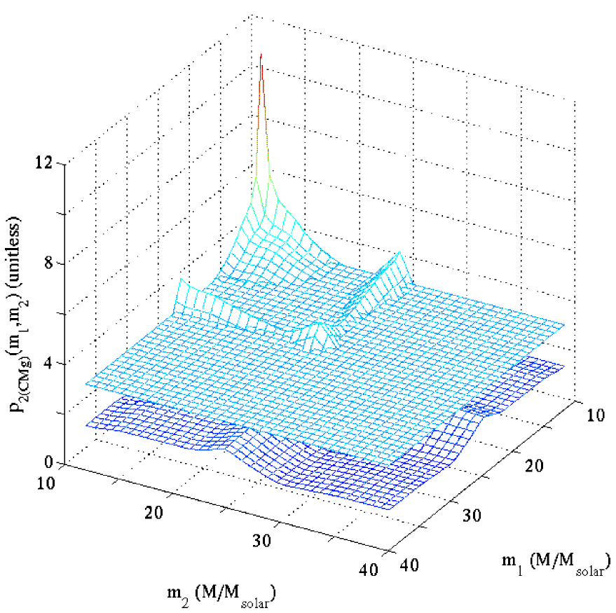
Figure 10: The two-dimensional yield ratio C/Mg as given by Eq. (16). Also shown in the figure is the plane at $p_{2\mathrm{(CMg)}}=3.50$. Every plane parallel to the $m_{1}m_{2}$-plane which intersects the yield function at a certain point defines an integration region for which the integral in Eq. (17) can be calculated, giving the value of the distribution function in the point $x=p_{2\mathrm{(CMg)}}$

It is worth mentioning a couple of properties of the convolution described by Eq. (14). When $n$ tends to infinity the corresponding density function of the arithmetical mean, i.e. the function derived from Eq. (39), tends to a Dirac delta function centred at $x=\int p(m)\phi(m)\mathrm{d}m$. Moreover, a sum of random variables can be approximated by a normal distribution according to the Central Limit Theorem. The dispersion of the arithmetical mean is then proportional to $n^{-1/2}$.

The number of SNe needed for this approximation to be valid depends ultimately on the shape of $f_{(A)}(x)$, but $n\sim 20$ is probably a good order-of-magnitude estimate. The averaging gradually erases the specific structures in the density functions and as soon as the shape of $f_{n(A)}(x)$ becomes well-behaved (i.e. Gaussian) it does not carry any information about the original yield and no new patterns are formed in the $A/$ diagrams (see, e.g., the decreasing scatter at the high-metallicity end in Fig. 3b or the crowding of stars round the point ($-0.19,-0.25$) in Fig. 5a).

4.2.3 Abundance ratios

In this section we shall derive the important expression for the distribution of an abundance ratio between two heavy elements, $A$ and $B$.

Let us first define a generalized stellar yield. The total amount of an element ejected by $n$ SNe can be regarded as a yield in the $n$-dimensional $m$-space, i.e.

$$p(m_{1},...,m_{n})=\sum\limits_{i=1}^{n}p(m_{i}),$$ (15)

where $p(m)$ is the normal, one-dimensional stellar yield for a star of mass $m$. In this way the yield ratio of two elements is simply defined as

$$p_{n(AB)}(m_{1},...,m_{n})=\frac{\sum\limits_{i=1}^{n}p_{(A)}(m_{i})}{\sum\limits_{i=1}^{n}p_{(B)}(m_{i})}.$$ (16)

As before, the subscript $n$ stands for the number of polluting SNe which in this case is equal to the number of dimensions as the original stellar yield is one-dimensional.

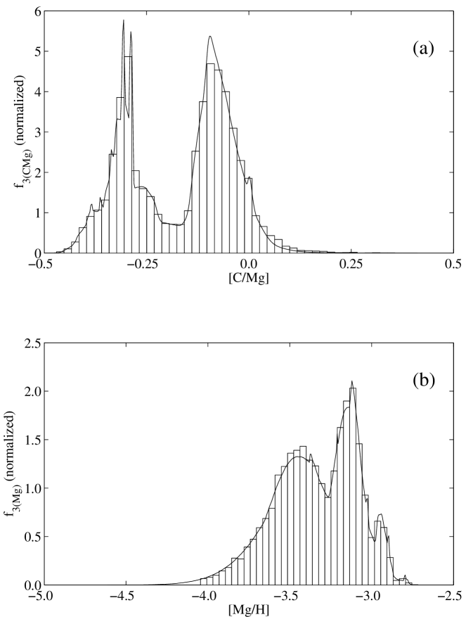
Figure 11: a) The density function of low mass-stars in [C/Mg]. Each star has been enriched by 3 SNe. Their masses were distributed according to the Salpeter IMF. As before, the histogram shows binned data from a numerical simulation while the full line is the corresponding density function to the formal solution of the distribution function in Eq. (17). b) The density function for [Mg/H]. This is in principle a convolution of the random variable $X_{\mathrm{(Mg)}}$ (see Fig. 9b) using Eq. (14) for $n=3$. The magnesium abundance is measured relative to $5\times 10^{5}\leavevmode\nobreak\ \mathcal{M_{\odot}}$ of hydrogen

Now, similarly to the multi-dimensional random variable in Eq. (32), we form the r.v. $X_{n(AB)}=p_{n(AB)}(M_{1},...,M_{n})$. This ratio has properties similar to that of the mean of a single element $A$. It is possible to show that the distribution function $F_{n(AB)}(x)$ can be written as

$$F_{n(AB)}(x)=\int...\int_{D_{x}}\phi(m_{1})\times...\times\phi(m_{n})\mathrm{d}m_{1}...\mathrm{d}m_{n}$$ (17)

according to Eq. (33). The integration region $D_{x}$ is defined by the equation

$$p_{n(AB)}(m_{1},...,m_{n})\leq x,$$ (18)

i.e. the part of the $m_{1}...m_{n}$-hyper plane where the yield is less than or equal to $x$ (see Fig. 10). Note that because all stellar mass r.v.s are independent the integrand in Eq. (33) reduces to a simple multiplication of the IMFs.

The integrand in Eq. (17) is almost trivial to handle while the integration region is highly non-trivial. From Eq. (18) we see that depending on how the yield varies, $D_{x}$ may not even be simply connected. This is illustrated in Fig. 10. The integral should be calculated for every $x$ which then gives the distribution function. The density function is obtained taking the derivative with respect to $x$ as in Eq. (13). Fig. 11 shows two examples of density functions of such compound random variables. Fig. 11a shows the distribution of stars over [C/Mg] for three polluting SNe using the same yields as above. The full line is a solution to Eq. (17). The density function in Fig. 11b is calculated from Eq. (14). Both functions are transformed to a logarithmic scale (and translated relative to solar values) using Eq. (40).

4.2.4 The construction of $A/$ diagrams

We are ultimately interested in two-dimensional distributions describing the density of extremely metal-poor low-mass stars in the $A/$ diagrams. If two random variables are independent their joint density equals the product of the individual densities (see the derivation of the convolution formula in Appendix A where independence is assumed). However, the random variables we discuss here are dependent. If we simultaneously observe the random variables in Fig. 11a and b the corresponding density function is not a multiplication of the two individual density functions. It is not possible to obtain every value of the ratio [C/Mg] for a given value of [Mg/H] by the combination of three SNe as the two variables are entangled via the progenitor masses of these SNe.

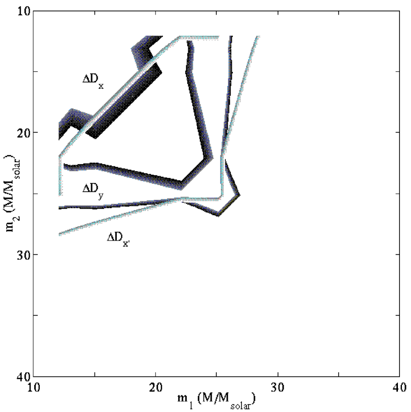
Figure 12: Intersecting integration regions. $\Delta D_{y}$ (dark-shaded areas) is defined by $p_{2\mathrm{(CMg)}}=y\sim 3.50$ (cf. Fig. 10) while $\Delta D_{x}$ and $\Delta D_{x^{\prime}}$ (light-shaded areas) are defined by $p_{2\mathrm{(Mg)}}=x\sim 0.10$ and $p_{2\mathrm{(Mg)}}=x^{\prime}\sim 0.20$ respectively. Hence, $\Delta D_{xy}$ and $\Delta D_{x^{\prime}y}$ are given by the intersections $\Delta D_{x}\bigcap\Delta D_{y}$ and $\Delta D_{x^{\prime}}\bigcap\Delta D_{y}$. A calculation of the integral in Eq. (19) over $\Delta D_{xy}$ for every $x=p_{2\mathrm{(Mg)}}(m_{1},m_{2})$ and $y=p_{2\mathrm{(CMg)}}(m_{1},m_{2})$ gives the two-dimensional density function $f_{2(\mathrm{Mg},\mathrm{CMg})}$

Suppose that we have four elements $A$, $B$, $C$, and $D$, where not all elements are necessarily different. Now, the joint distribution of $X_{n(AB)}$ and $X_{n(CD)}$ (or, e.g., $X_{n(A)}$ and $X_{n(BC)}$) is described by the function $f_{n(AB,CD)}$ (or$f_{n(A,BC)}$). As usual, the subscript $n$ stands for the number of contributing SNe. The derivation is similar to that of the one-dimensional distribution function in Eq. (17). Here, the density functions are calculated directly, as in Eq. (38). Thus,

$$f_{n(AB,CD)}(x,y) = \int...\int_{\Delta D_{xy}}\phi(m_{1})\times...$$ (19)

$$\times \phi(m_{n})\mathrm{d}m_{1}...\mathrm{d}m_{n},$$

where the integration region, $\Delta D_{xy}$ is defined via the equations

$$\left\{\begin{array}[]{ll}\Delta D_{x}:\leavevmode\nobreak\ x<p_{n(AB)}(m_{1},...,m_{n})\leq x+\mathrm{d}x\\ \Delta D_{y}:\leavevmode\nobreak\ y<p_{n(CD)}(m_{1},...,m_{n})\leq y+\mathrm{d}y.\end{array}\right.$$ (20)

Thus, for every point $(x,y)$ the integration is performed over the small common region in $m$-space defined by the intersection, $\Delta D_{x}\bigcap\Delta D_{y}$. The density of stars (enriched by $n$ SNe) in the [$A$/H]–[$B$/$C$] plane, described by $f_{n(A,BC)}(x,y)$, is calculated similarly. However, the integration region is changed to (see Fig. 12)

$$\left\{\begin{array}[]{ll}\Delta D_{x}:\leavevmode\nobreak\ x<p_{n(A)}(m_{1},...,m_{n})\leq x+\mathrm{d}x\\ \Delta D_{y}:\leavevmode\nobreak\ y<p_{n(BC)}(m_{1},...,m_{n})\leq y+\mathrm{d}y.\end{array}\right.$$ (21)

The integrands in Eq. (17) and Eq. (19) are the same. The difference lies again in the integration regions and we note that the (generalized) stellar yields are important components in the expression for the abundance ratio as the functions defining these regions. Moreover, the IMF only partly determines the density in each point, together with the gradient of the yield function. This is clearly seen in Eq. (13) but can also be traced in Fig. 12 where the differential areas have different sizes depending on the shape of the yields.

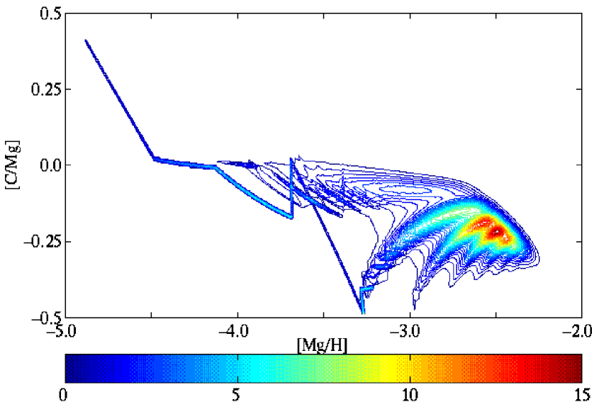
Figure 13: Contour plot of $f_{\mathrm{Mg},\mathrm{CMg}}$ (cf. Fig. 3a) computed for 1–20 SNe with $w_{i}=1/20=0.05$ using the yields from WW95. The IMF is of Salpeter form. The relative number density of stars is indicated by the colour bar

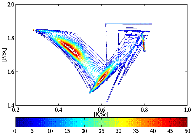
Figure 14: Contour plot of $f_{\mathrm{KSc},\mathrm{PSc}}$. The model parameters are the same as in Fig. 13. The stellar yields are taken from Netal97. The colour bar indicates the relative number density of stars

The final step to an analytical expression for the distribution of stars in an $A/$ diagram is a summation of the density functions over the number of SNe. The expression for the density in an $A/A$ diagram, i.e. the density in the [$A$/$B$]–[$C$/$D$] plane, is

$$f_{AB,CD}(x,y)=\sum\limits_{i=1}^{n}w_{i}\times f_{i(AB,CD)}(x,y).$$ (22)

The weight $w_{i}$ is the fraction of clouds forming $i$ SNe. If we substitute $f_{i(A,BC)}(x,y)$ in the sum, we instead obtain a function formally describing the density of stars in the [$A$/H]–[$B$/$C$] plane. Note that the first term in the sum is a one-dimensional function since any star enriched by a single SN has a unique chemical composition determined by the yields of that SN. Thus, the density function maps the one-dimensional yield ratio on the $A/A$ plane. The function is seen as a curve in Figs. 13 and 14 (see also Fig. 8). The form of this curve actually determines the form of the total density function to a large extent.

We end this section by a small note on scale transformations. The appropriate equations are derived in Appendix A. In our derivations all functions are on a linear scale. Often astrophysical quantities may span several orders of magnitude. It is then more advantageous to display these quantities on a logarithmic scale. The transformation is made using Eq. (40) and Eq. (41) for one- and two-dimensional functions respectively. However, it is also possible to directly take the logarithm of the yield or the generalized yield and use these functions in the expressions for the densities instead.

4.3 The robustness of the $A/A$ diagrams

It is not probable that patterns like those in Fig. 13 can be observed, since they are based on oversimplified models. The star-forming regions have different masses. Mixing within the regions is not complete and global mixing of remnant, enriched gas, or infalling gas, and the formation of a second generation of star-forming regions probably occurred even for the extremely metal-poor Halo. By neglecting all these effects the treatment of the mixing in our models is oversimplified (see Nakasato & Shigeyama 2000). Thus, a horizontal smearing effect occurs in $A/$H diagrams such as [Mg/H]–[C/Mg], and the patterns are most likely lost in these diagrams.

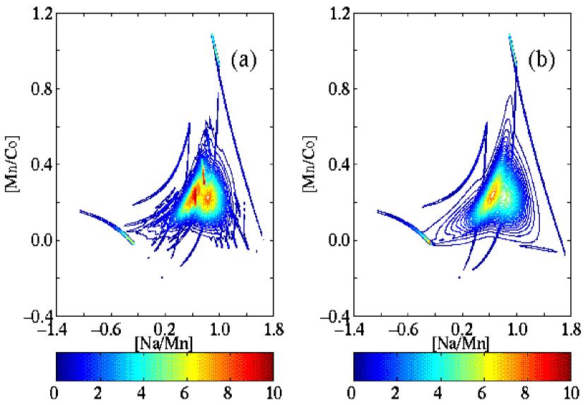
Figure 15: Contour plots of the density of stars in the [Na/Mn]–[Mn/Co] plane with yields from Netal97. a) The density function with unweighted yield terms (i.e. $\xi_{i}=1$ for all $i$). b) The corresponding function with weighted yield terms according to Eq. (23) representing the effect of global mixing. The weights have a uniform distribution, ranging from $0$ to $1$. Due to the weights the microstructure in the second $A/A$ diagram has been wiped out. Otherwise, the difference between the two diagrams is very small

The patterns in the $A/A$ diagrams are, however, not sensitive to the masses of the star-forming regions, i.e. the amount of ambient gas that is mixed with the SN ejecta. If the SN remnant material is mixed with a pre-enriched ISM one might yet think that the information on the original production sites of the elements can not be traced in the observed abundance ratios, as different fractions of the enriched medium may contribute differently to different stars. This occurs when a second generation of star-forming regions is formed. Suppose for example that a new region is formed out of the dispersed gas of two former such regions with the proportions $1:3$, i.e. $25\%$ of the total mass originates from the first region and $75\%$ of the mass from the second region. Assume further that these former regions were enriched by one SN each and the new region produces one SN. An abundance ratio in the gas and in subsequently formed stars is then found by summing up the individual contributions from each SN, as in Eq. (16). However, each term has a a weight associated with it, depending on how great the contribution is from each region. In our example the weights are $0.25,\leavevmode\nobreak\ 0.75$ and $1.00$. Generally, Eq. (16) has to be modified such that

$$p^{\xi}_{n(AB)}(m_{1},...,m_{n})=\frac{\sum\limits_{i=1}^{n}\xi_{i}p_{(A)}(m_{i})}{\sum\limits_{i=1}^{n}\xi_{i}p_{(B)}(m_{i})}.$$ (23)

The only difference between this expression and the one in Eq. (16) is the weight $\xi_{i}$ on each yield. The weight is supposed to mimic the effect of large-scale mixing and turbulent motions in the ISM and can be regarded as a random variable similar to the mass such that the r.v. $X^{\xi}_{n(AB)}$ is

$$X^{\xi}_{n(AB)}=\frac{\sum\limits_{i=1}^{n}\Xi_{i}p_{(A)}(M_{i})}{\sum\limits_{i=1}^{n}\Xi_{i}p_{(B)}(M_{i})}=p^{\xi}_{n(AB)}(\Xi_{1},M_{1},...,\Xi_{n},M_{n})$$ (24)

where the superscript $\xi$ denotes the fractional contribution defined by the weighted generalized yields in Eq. (23). By introducing these weights, the generalized yield $p_{n(AB)}(m_{1},...,m_{n})$ looses its symmetry (e.g. in Fig. 10, the two-dimensional yield ratio would no longer be symmetric around $m_{1}=m_{2}$). Thus, depending on the weights, a specific abundance ratio may be produced by several different sets of SNe. This means that if we have no information on the weights we are no longer able to identify the set of SNe that gives the observed ratio.

Even so, simulations with randomly distributed weights show that the distribution of stars in $A/A$ diagrams is practically unaltered (see Fig. 15) with respect to the original distribution for which all $\xi_{i}=1$. This is due to the fact that the intersection between the two regions $\Delta D_{x}^{\xi}$ and $\Delta D_{y}^{\xi}$ is non-zero (thus, the integral in Eq. (19) is non-zero) in almost the same region in yield space (i.e. abundance ratio space) as for the unperturbed (unweighted) integration region $\Delta D_{xy}$. Note however, that the integration region over stellar masses may be different and far from symmetric which changes the value of the density function in each point. This is also observed in Fig. 15. The distributions have the same shape but the density of stars in the structures is somewhat different. Furthermore, in Fig. 15b the microstructure is wiped out. It is clear that some information must be lost by introducing weights on the yield terms. Thus, we have no longer knowledge of the absolute amounts of the elements produced in the SNe.

Even though the two chemical patterns in Fig. 15 look qualitatively similar a relevant question is whether the microstructure in Fig. 15a is crucial for a reconstruction of SN yields. This structure originates from the one-dimensional curve sampling individual SNe (cf. the red curves in the diagrams of Fig. 8) or sooner it corresponds to this curve for the case $n=2,3,$ etc. In principle, this structure does not contain any unique information and the loss of it should not be vital for a yield reconstruction procedure. In this particular example the pattern in Fig. 15a also shows two distinct peaks of which the right one is the convergence point or the centre of gravity. This dichotomy is not as prominent in Fig. 15b. Would the lack of a second peak lead to a significantly different result when reconstructing the yields? We believe that this is not the case. A comparison with the much greater diversity of patterns shown in Fig. 5 suggests that the major part of the information content on the yields in Fig. 15a still remains in Fig. 15b. A number of similar simulations for other elements confirm this result. However, more tests should be carried out in order to quantitatively determine the sensitivity of the yields on the details of the chemical patterns.

5 Discussion – Can patterns be observed?

Above, we have discussed the formation of patterns in $A/$ diagrams and the possibilities of using abundance ratios as a diagnostic of early stellar nucleosynthesis. However, the question remains: Are chemical abundance patterns detectable in practice?

It is difficult to estimate the accuracy needed in the abundance determinations and the minimum number or sample stars that is required for detecting the chemical patterns. Since the number of Halo stars that can be observed accurately is limited, these parameters are dependent. Fig. 16 shows a comparison between the original distribution of about $100$ stars in the [K/Sc]-[P/Sc] plane (cf. Fig. 14) and the corresponding distribution for which an uncertainty of $0.08$ dex is added in the observed abundance ratios. The original ”V”-shape is barely detected in Fig. 16b. However, the pattern would more easily appear if we could double the number of stars. Larger uncertainties in the abundance ratios would completely wipe out the pattern and this can not be compensated for by adding more stars. On the other hand, the ”U”-shape in Fig. 5c is detectable even for uncertainties above $0.1$ dex in the abundance ratios. However, for making that pattern visible at all several hundred stars must be observed, many more than are needed for the ”V”-shaped pattern. Thus, depending on the shape, some patterns are more sensitive to observational uncertainties than to the number of sample stars while the opposite is true for other types of patterns.

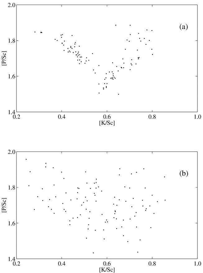
Figure 16: a) A scatter plot of around $100$ stars (enriched by $1$–$15$ SNe) in the [K/Sc]–[P/SC] plane. The nucleosynthesis calculations by Netal97 have been used. The ”V”-shape is easily detected (cf. Fig. 14). b) The corresponding distribution with an additional uncertainty of $0.08$ dex in the abundance ratios. The ”V”-shape is less pronounced but still detectable

This discussion also holds for $A/$H diagrams (e.g. Fig. 3). Assuming that there are no intrinsic uncertainties which wipe out the patterns, we estimate, by convolving the density function in Fig. 13 with a Gaussian profile, that the structures become undetectable if the uncertainties in the derived abundances are larger than $\sim 0.05$ dex. This is an upper limit as we in reality only deal with a limited number of sample stars, i.e. poorer statistics. However, e.g., the bimodal structure in the [N/O]–[O/H] plane (see Fig. 3 in Karlsson & Gustafsson 2000) caused by a pronounced peak in the N-yield (WW95) is not erased even for uncertainties in the abundances as large as $0.15$ dex. This also suggests that large-scale structures in $A/$H diagrams can possibly survive the effect of mixing in the interstellar medium, if the mass range of typical star-formation regions is limited to within a factor of $2$ or so. One should also note that similar patterns could also be expected to be visible in smaller star systems enriched by a finite number of SNe with full mixing of the system occurring between each SN.

Observing chemical patterns will be a challenging task. With the tools of today and current methods for abundance analysis we are able to decrease the absolute observational uncertainties in the abundance ratios to $\sim 0.1$ dex. A strictly differential study may reach the $0.05$ dex level of uncertainty. This may be slightly too large to allow detection of the fine-structures in many patterns which seem to begin appearing first at a level of about $0.05$ dex. However, larger uncertainties can, as we have seen, partly be compensated for by a larger stellar sample. Also, in a number of cases patterns should be visible already with errors in the relative abundances of $\sim 0.1$ dex.

5.1 Existing evidence for chemical patterns

Our aim is here not to make a literature survey of abundance data for metal-poor stars or to re-analyse existing data but merely to point out some studies and phenomena that possible can be related to variations in stellar yields and the formation of chemical patterns.

There may be undetected patterns in the sample of some thirty metal-poor giants ([Fe/H]$<-2$) observed by McWilliam et al. (1995). The sample is fairly homogeneous although the stars are not dwarfs and internal nucleosynthesis may have altered some of their surface abundances. Nevertheless, let us look at the distribution of stars in the [Mg/Fe]–[C/Mg] plane which is shown in Fig. 17. The symbols are shaded according to the stellar metallicity as measured by [Fe/H]. The dispersion is large in both directions, spanning $1.5$ dex in [Mg/Fe] and nearly $3$ dex in [C/Mg]. The distribution of stars is asymmetric and there is no strong correlation with metallicity. However, there are too few stars in the sample to really allow the detection of any patterns.

If we instead plot the stars in the [C/Ca]–[C/Mg] plane, we find something completely different. The stars form a quite beautiful relation (see Fig. 18). The slope is close to unity and there seems to be no direct dependence on the iron abundance as indicated by the shading of the star symbols. In accordance with our discussion on early chemical enrichment we shall assume that these stars have been enriched by a small number of core collapse supernovae at the epoch of formation of the Galaxy. If so, this leads us to believe that, whatever the variation of the yields with SN mass is, the ratio of the Ca-yield to the Mg-yield is rather independent of progenitor mass. The scaling factor (by number relative to solar values) can directly be estimated from the offset in Fig. 18 and gives $N_{\mathrm{Ca}}\simeq 1.15N_{\mathrm{Mg}}$ although it is consistent with unity. This relation can also be observed in the [Fe/H]–[Ca/Mg] plane where the stars are scattered around the constant value of $0.06$. The scaling relation between the yields (by mass) is then estimated to $p_{\mathrm{Ca}}(m)\simeq 0.1p_{\mathrm{Mg}}(m)$. Only weak observational constraints on the carbon yield can be deduced from the diagram in Fig. 18. However, the observed abundance ratios span almost three orders of magnitude which is considerable.

Recently, Jehin et al. (1999) observed a sample of mildly metal-poor stars and found interesting correlations between the abundances of the $\alpha$-elements and the r- and s-process elements. The $\alpha$-elements were correlated with the r-process elements in a one-to-one relation while a subpopulation of the stars with high [$\alpha$/Fe] ratio seemed to be enriched in the s-process elements (see their Fig. 7). This excess in s-process elements was interpreted as an accretion phenomenon in dense environments, presumably globular clusters. We note that their correlation diagrams show strong similarities with some of the $A/A$ diagrams presented here, see Fig. 6a and Fig. 7. There is little doubt that the reversed ”L”-shape and their two-branches-pattern are both caused by strong variations in the stellar yields. However, it is not clear whether the two-branches-pattern could be explained by yield variations alone or if an evolutionary effect is necessary as proposed by these authors.

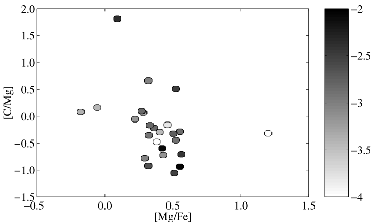
Figure 17: Observed abundances of stars from McWilliam et al. (1995) displayed in the [Mg/Fe]–[C/Mg] plane (cf. Figs. 5a and 5d). The shading according to the bar on the right indicates the metallicity measured by [Fe/H]. Stars with $B-V>0.80$ are removed from the sample in order to minimize the effect of carbon depletion in the red giants. There are too few stars to allow detection of any patterns although there seems to be a large, asymmetric dispersion

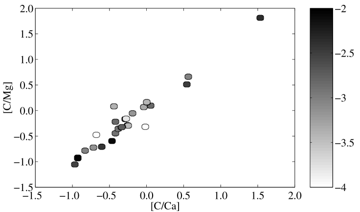
Figure 18: Abundances of stars from the sample of McWilliam et al. (1995) plotted in the [C/Ca]–[C/Mg] plane. As for Fig. 17, the symbols are shaded according to the stellar metallicity. Stars with $B-V>0.80$ have been removed from the sample. Note that the observed stars form a tight relation with a slope close to one

Another possibly related phenomenon is the existence of CN-strong and CN-weak line stars in some globular clusters (see e.g. Cannon et al. 1998). There seems to be a distinct bimodal abundance pattern in this population of stars, not much different from patterns formed by a yield with a pronounced maximum. The bimodality in the CN line strengths is not yet understood but, again, strong variations in the yields would produce similar patterns. We should emphasize that our discussion on the formation of patterns only holds in a strict sense for extremely metal-poor environments while the latter two examples concern relatively metal-rich systems.

6 Conclusions

Observations of the most metal-poor Galactic halo stars show convincing evidence for a large star-to-star scatter in abundances relative to hydrogen as well as abundance ratios for a variety of elements, not the least the neutron-capture elements (McWilliam et al. 1995; Ryan et al. 1996; McWilliam 1998; Burris et al. 2000). This phenomenon can most easily be explained in terms of local enrichment of the primordial ISM by a small number of exploding massive stars (Audouze & Silk 1995). Since the amounts of newly synthesized elements depend strongly on the mass of the exploding star (some elements are also affected by parameters such as rotation and metallicity), the abundances might have varied extensively throughout the Halo ISM. Before turbulent motions in the ISM had time to wipe out the chemical inhomogeneities, formation of low-mass stars occurred and the inhomogeneities could be preserved. Hence, studying these stars by statistical means, especially by displaying them in $A/A$ diagrams relating different abundance ratios, reveals important information on the production sites of the elements.

We have demonstrated that a sample of extremely metal-poor stars displayed in $A/$ diagrams forms patterns which originate from specific variations in the stellar yields. Thus, the formation of patterns is a natural consequence of the variations in the amount of SN-produced material. This is clearly seen in the analytical theory. The form of the patterns depend critically on the shape of the integration regions which are defined by the SN yields. Furthermore, assuming that the ejected matter from SN explosions can be considered chemically homogeneous (see e.g. Kifonidis et al. 2000; see also the comment by Arnett 1999) we claim, based on the result given in Sect. 4.3, that chemical abundance patterns in $A/A$ diagrams (such as [C/Mg] vs. [Mg/Fe]) survive the effects of large-scale mixing in the ISM (see Fig. 15). Moreover, a comparison between the simulations of Model I and Model II (cf. Fig. 5 and Fig. 6) indicates that the patterns are not very sensitive to the mass distribution function of exploding SNe (see also Fig. 3 in Karlsson & Gustafsson 2000). In the analytical expression the mass distribution function appears in the integrand. Hence, it merely specifies the relative density of stars within the patterns, not the form of the patterns. For a finite stellar sample, however, the apparent form of the patterns will depend slightly on the mass frequency of SNe since a finite number of stars do not cover all possible values defined by the theoretical density function.

Continuous star formation within the clouds (Model II) could modify the chemical patterns. However, such an evolutionary effect would result in a displacement of the centre of gravity rather than the formation of new patterns. The number of contributing SNe in individual star-forming regions must be large ($>20$) in order to detect the displacement (cf. Figs. 5c, 5e and Fig. 6) and it vanishes for stars formed in a second generation of star-forming regions. The general characteristics of the patterns are, however, not affected (see Sect. 4.3).

In comparison to studies of individual Halo stars with dramatic abundance signatures like CS 22892-052, the inclusion of less extreme stars makes it possible to quantitatively discriminate between chemical patterns formed by different SN yields (see Fig. 5). Future prospects include studies of large, homogeneous samples of extremely metal-poor Halo stars with accurately determined abundance ratios. In fact, several surveys of this kind are already under way. The idea would be to reconstruct the yields by solving the inverse problem. An observed chemical pattern in some $A/A$ plane is compared with simulations whereupon the yields are changed until the two distributions are, in some sense, equal. Some potential complications are noted. The possible contamination of thermonuclear SNe (SNe type Ia), intermediate-mass stars, and/or very massive stars might affect the chemical patterns and blur the nucleosynthetic signature of the core collapse SNe. Metallicity dependent yields affect the patterns of secondary elements. However, we estimate that for the first generations of extreme Pop. II stars, and for several elements, the contamination should not be very severe. The development of more realistic, time-dependent models should elucidate these problems, as well as those of mixing on various spatial and temporal scales. In a forthcoming paper we shall present a general method for SN-yield reconstruction.

A quantitative analysis is possible only if the SN yields can be strictly parametrized. In particular, the explosive nucleosynthesis is a product of a chaotic behaviour of the stellar material, intimately connected to hydrodynamical instabilities. Shocks, convection and turbulent motions in the SN gas could introduce intrinsic uncertainties in the produced amount of elements. The stochastic nature of such an effect could blur the chemical patterns in the $A/$ diagrams. However, if the effect is sufficiently small it should be possible to retrieve mean yields as functions of mass, rotation etc. We conclude that the chemical patterns are useful diagnostics of yields of core collapse SNe, and if patterns would be detected, we would have the opportunity to probe the earliest phases of stellar nucleosynthesis.

Appendix A

The analytical treatment of the stellar distributions in the $A/$ diagrams (Sect. 4) is developed in order to form a deeper understanding of the parameter dependence of the observed patterns. Here, we shall derive some general expressions for density functions as well as distribution functions corresponding to an arbitrary random variable or pairs of random variables. Note, that in Sect. 4.2 we wrote the random variables in the subscripts within parentheses. This notation was adopted for purposes explained in the text. However, this in not the conventional notation, and in this section the subscripts are written without parentheses.

A.1 Functions of one random variable

Suppose we have a random variable (r.v.) $X$ and a function $y=g(x)$. Assume this function to be monotonically increasing with increasing $x$. Now, define the r.v. $Y$ as $Y=g(X)$. The probability that $Y\leq y$ is then given by the distribution function for $Y$,

$$F_{Y}(y) = P(Y\leq y)=P(g(X)\leq y)=$$ (25)

$$= P(X\leq g^{-1}(y))=F_{X}(g^{-1}(y)),$$

where $F_{X}$ is the distribution function of the r.v. $X$. The inverse function of $g$ is denoted by $g^{-1}$. For a monotonically decreasing function $g$ we will have that $F_{Y}(y)=1-F_{X}(g^{-1}(y))$ instead.

In the continuous case the corresponding density function of $Y$ is given by the derivative of $F_{Y}(y)$ with respect to $y$ such that

$$f_{Y}(y)=F_{X}^{\prime}(g^{-1}(y))=f_{X}(g^{-1}(y))\left|\frac{\mathrm{d}}{\mathrm{d}y}g^{-1}(y)\right|.$$ (26)

We can allow the function $g$ to be non-monotonic by defining it as a sum, $g=g_{1}+...+g_{n}$ where each function $g_{i}$ is monotonic and equivalent to $g$ on the open subinterval ]$x_{i-1},x_{i}$[ and zero elsewhere. The $x_{i},\leavevmode\nobreak\ i=1,...,n-1$ are real roots of $g^{\prime}(x)$ and $x_{0},\leavevmode\nobreak\ x_{n}$ are the end-points. Thus, similarly to Eq. (26) the expression for $f_{Y}(y)$ reads

$$f_{Y}(y) = \frac{\mathrm{d}}{\mathrm{d}y}F_{Y}(y)=\sum\limits_{i=1}^{n}\left|\frac{\mathrm{d}}{\mathrm{d}y}\left(g_{i}^{-1}(y)\right)\right|f_{X}(g_{i}^{-1}(y))=$$ (27)

$$= \sum\limits_{i=1}^{n}\frac{f_{X}(g_{i}^{-1}(y))}{\left|g_{i}^{\prime}(g_{i}^{-1}(y))\right|},$$

where $g^{\prime}\equiv\mathrm{d}g/\mathrm{d}x$.

A.2 The convolution formula

Given two continuous random variables, $Y$ and $Z$, with distribution functions $F_{Y}$ and $F_{Z}$ respectively, the sum, $X=Y+Z$, is described by the distribution function $F_{X}$ given by the integral,

$$F_{X}(x)=\int\!\!\!\int_{y+z\leq x}f_{Y,Z}(y,z)dydz.$$ (28)

If $Y$ and $Z$ are independent Eq. (28) reduces to

$$F_{X}(x)=\int\!\!\!\int_{y+z\leq x}f_{Y}(y)f_{Z}(z)dydz.$$ (29)

This expression can be rewritten as

$$F_{X}(x) = \int\limits_{-\infty}^{+\infty}f_{Y}(y)\left[\int\limits_{-\infty}^{x-y}f_{Z}(z)dz\right]dy=$$ (30)

$$= \int\limits_{-\infty}^{+\infty}f_{Y}(y)F_{Z}(x-y)dy.$$

The derivative of $F_{X}(x)$ with respect to $x$ gives the density function,

$$f_{X}(x)=\int\limits_{-\infty}^{+\infty}f_{Y}(y)f_{Z}(x-y)dy$$ (31)

(assuming that derivation under the integral sign is allowed). Eq. (31) is the convolution formula for two continuous and independent random variables.

A.3 One- and two-dimensional distributions of $n$ random variables

In this section, we shall form expressions for one-dimensional density functions of $n$ continuous random variables as well as two-dimensional density functions of $n$ random variables.

Given $n$ random variables $X_{1},...,X_{n}$ and a real-valued function $g=g(x_{1},...,x_{n})$ we may form the one-dimensional r.v.

$$X=g(X_{1},...,X_{n}).$$ (32)

For every given number $x$, we denote by $D_{x}$ the region in the $x_{1}...x_{n}$ hyper-plane such that $g(x_{1},...,x_{n})\leq x$. Hence, the distribution function of $X$ is given by the integral

$$F_{X}(x) = P(X\leq x)=P((X_{1},...,X_{n})\in D_{x})=$$ (33)

$$= \int...\int_{D_{x}}f_{X_{1},...,X_{n}}(x_{1},...,x_{n})\mathrm{d}x_{1}...\mathrm{d}x_{n},$$

where $f_{X_{1},...,X_{n}}(x_{1},...,x_{n})$ is the density function of the joint distribution of $X_{1},...,X_{n}$. The corresponding density function of the r.v. $X$ is simply given by the derivative of the distribution function $F_{X}(x)$, as in Eq. (26).

Clearly, Eq. (33) is in particular valid in the one-dimensional case. Namely, if that $y=g(x)$ is a monotonically increasing function, then Eq. (33) reduces to Eq. (25).

Again, suppose that we have $n$ random variables. It is then possible to define two new r.v.s $X$ and $Y$ via the functions $g(x_{1},...,x_{n})$ and $h(x_{1},...,x_{n})$ such that

$$X=g(X_{1},...,X_{n}),\leavevmode\nobreak\ \leavevmode\nobreak\ \leavevmode\nobreak\ \leavevmode\nobreak\ \leavevmode\nobreak\ \leavevmode\nobreak\ \leavevmode\nobreak\ \leavevmode\nobreak\ \leavevmode\nobreak\ \leavevmode\nobreak\ Y=h(X_{1},...,X_{n}).$$ (34)

The expression for the joint distribution of $X$ and $Y$ is similar to that of Eq. (33). However, we shall directly express the density function $f_{X,Y}(x,y)$ by defining the integration region as an intersection between the two differential integration regions $\Delta D_{x}$ and $\Delta D_{y}$,

$$\{x<X\leq x+\mathrm{d}x\}=\{(X_{1},...,X_{n})\in\Delta D_{x}\}$$ (35)

and

$$\{y<Y\leq y+\mathrm{d}y\}=\{(X_{1},...,X_{n})\in\Delta D_{y}\}.$$ (36)

Note, that the density function of $X$, defined by Eq. (32), can be calculated directly by substituting $\Delta D_{x}$ for $D_{x}$ in the integral in Eq. (33). Now, for calculating the joint statistics of $X$ and $Y$ we introduce $\Delta D_{xy}=\Delta D_{x}\bigcap\Delta D_{y}$, or

$$\{x<X\leq x+\mathrm{d}x,\leavevmode\nobreak\ y<Y\leq y+\mathrm{d}y\} =$$

$$=\{(X_{1},...,X_{n})\in\Delta D_{xy}\}$$ (37)

Finally, we then have

$$f_{X,Y}(x,y) =$$ (38)

$$= P(x<X\leq x+\mathrm{d}x,y<Y\leq y+\mathrm{d}y)=$$

$$= P((X_{1},...,X_{n})\in\Delta D_{xy})=$$

$$= \int...\int_{D_{xy}}f_{X_{1},...,X_{n}}(x_{1},...,x_{n})\mathrm{d}x_{1}...\mathrm{d}x_{n}.$$

A general treatment of multi-variate distributions is discussed in e.g. Papoulis (1991). Further reading on the theory of probability can also be found in Gut (1995).

A.4 Some scaling laws

In connection to Sect. 4.2.2 and Eq. (14) we would also like to consider a density function describing the mean of r.v.s instead of the sum. With a simple scaling $f_{nX}(x)$ is transformed into

$$f_{\langle nX\rangle}(x)=nf_{nX}(nx),$$ (39)

where the subscript $\langle nX\rangle$ on $f$ denotes the average of $n$ random variables.

All functions in Sects. 4.2 and 4.3 are displayed on a logarithmic scale. Using Eq. (25) and Eq. (27) with $g(X)=\log(X)$ we see that an arbitrary function of one variable transforms as

$$f_{{\log X}}(x)=\ln(10)\times 10^{x}f_{X}(10^{x}).$$ (40)

The factor $\ln(10)$ arises from the fact that we use the 10-logarithm, not the natural logarithm. Similarly, a two-dimensional function transforms as,

$$f_{\log X,\log Y}(x,y)=\ln^{2}(10)\times 10^{x+y}f_{X,Y}(10^{x},10^{y}).$$ (41)

However, instead of calculating the densities on a linear scale and then make the transformations, it is easier to directly take the logarithm of the generalized yields and use these functions in the calculations.

References

- Argast et al. (2000) Argast, D., Samland, M., Gerhard, O. E., & Thielemann, F. K. 2000, A&A, 356, 873
- Arnett (1999) Arnett, D. 1999, Ap&SS, 265, 29
- Audouze & Silk (1995) Audouze, J., & Silk, J. 1995, ApJ, 451, L49
- Binney & Merrifield (1998) Binney, J., & Merrifield, M. 1998, Galactic Astronomy (Princeton University Press, Princeton)
- Branch (1998) Branch, D. 1998, ARA&A, 36, 17
- Burris et al. (2000) Burris, D. L., Pilachowski, C. A., Armandroff, T. E., et al. 2000, ApJ, 544, 302
- Cannon et al. (1998) Cannon, R. D., Croke, B. F. W., Bell, R. A., Hesser, J. E., & Stathakis, R. A. 1998, MNRAS, 298, 601
- Christlieb & Beers (2000) Christlieb, N., & Beers, T. C. 2000, in HDS Workshop, Proc. of the Subaru HDS workshop, ed. M. Takada-Hidai, & H. Ando, 255 (astro-ph/0001378)
- Douvion et al. (1999) Douvion, T., Lagage, P. O., & Cesarsky, C. J. 1999, A&A, 352, L111
- Edvardsson et al. (1993) Edvardsson, B., Andersen, J., Gustafsson, B., et al. 1993, A&A, 275, 101
- Gustafsson et al. (1999) Gustafsson, B., Karlsson, T., Olsson, E., Edvardsson, B., & Ryde, N. 1999, A&A, 342, 426
- Gut (1995) Gut, A. 1995, An Intermediate Course in Probability (Springer-Verlag, New York)
- Heger & Langer (2000) Heger, A., & Langer, N. 2000, ApJ, 544, 1016
- Henry et al. (2000) Henry, R. B. C., Edmunds, M. G., & Köppen, J. 2000, ApJ, 541, 660
- Hughes et al. (2000) Hughes, J. P., Rakowski, C. E., Burrows, D. N., & Slane, P. O. 2000, ApJ, 528, L109
- Ishimaru & Wanajo (1999) Ishimaru, Y., & Wanajo, S. 1999, ApJ, 511, L33
- Jehin et al. (1999) Jehin, E., Magain, P., Neuforge, C., et al. 1999, A&A, 341, 241
- Karlsson & Gustafsson (2000) Karlsson, T., & Gustafsson, B. 2000, in The Galactic Halo: from Globular Clusters to Field Stars, ed. A. Noels, P. Magain, D. Caro, et al., 237
- Kifonidis et al. (2000) Kifonidis, K., Plewa, T., Janka, T. T., & Müller, E. 2000, ApJ, 531, L123
- Maeder (1992) Maeder, A. 1992, A&A, 264, 105
- McWilliam (1998) McWilliam, A. 1998, AJ, 115, 1640
- McWilliam et al. (1996) McWilliam, A., Preston, G., Sneden, C., Searle, L., & Shectman, S. 1996, in ASP Conf. Ser. 92: Formation of the Galactic Halo… Inside and Out, 317
- McWilliam et al. (1995) McWilliam, A., Preston, G. W., Sneden, C., & Searle, L. 1995, AJ, 109, 2757
- Nakasato & Shigeyama (2000) Nakasato, N. & Shigeyama, T. 2000, ApJ, 541, L59
- Nissen et al. (1994) Nissen, P.-E., Gustafsson, B., Edvardsson, B., & Gilmore, G. 1994, A&A, 285, 440
- Nomoto et al. (1997) Nomoto, K., Hashimoto, M., Tsujimoto, T., et al. 1997, Nucl. Phys. A, 616, 79 (Netal97)
- Pagel (1997) Pagel, B. E. J. 1997, Nucleosynthesis and Chemical Evolution of Galaxies (Cambridge University Press, Cambridge)
- Papoulis (1991) Papoulis, A. 1991, Probability, Random Variables, and Stochastic Processes, 3rd edn. (McGraw-Hill, New York)
- Portinari et al. (1998) Portinari, L., Chiosi, C., & Bressan, A. 1998, A&A, 334, 505
- Raiteri et al. (1999) Raiteri, C. M., Villata, M., Gallino, R., Busso, M., & Cravanzola, A. 1999, ApJ, 518, L91
- Ryan et al. (1996) Ryan, S. G., Norris, J. E., & Beers, T. C. 1996, ApJ, 471, 254
- Shull & Saken (1995) Shull, J. M., & Saken, J. M. 1995, ApJ, 444, 663
- Sneden et al. (1996) Sneden, C., McWilliam, A., Preston, G. W., et al. 1996, ApJ, 467, 819
- Suzuki et al. (1999) Suzuki, T. K., Yoshii, Y., & Kajino, T. 1999, ApJ, 522, L125
- Travaglio et al. (2001) Travaglio, C., Galli, D., & Burkert, A. 2001, ApJ, in press (astro-ph/0009165)
- Travaglio et al. (1999) Travaglio, C., Gallino, R., Amari, S., et al. 1999, ApJ, 510, 325
- Tsujimoto & Shigeyama (1998) Tsujimoto, T., & Shigeyama, T. 1998, ApJ, 508, L151
- Tsujimoto et al. (2000) Tsujimoto, T., Shigeyama, T., & Yoshii, Y. 2000, ApJ, 531, L33
- Umeda et al. (2000) Umeda, H., Nomoto, K., & Nakamura, T. 2000, in The First Stars, Proc. of the MPA/ESO workshop, ed. A. Weiss, T. G. Abel, & V. Hill, 137
- Wasserburg & Qian (2000) Wasserburg, G. J., & Qian, Y.-Z. 2000, ApJ, 529, L21
- Woosley & Weaver (1995) Woosley, S. E., & Weaver, T. A. 1995, ApJS, 101, 181 (WW95)