Robustness of the Quintessence Scenario in Particle Cosmologies

Abstract

We study the robustness of the quintessence tracking scenario in the context of more general cosmological models that derive from high-energy physics. We consider the effects of inclusion of multiple scalar fields, corrections to the Hubble expansion law (such as those that arise in brane cosmological models), and potentials that decay with expansion of the Universe. We find that in a successful tracking quintessence model the average equation of state must remain nearly constant. Overall, the conditions for successful tracking become more complex in these more general settings. Tracking can become more fragile in presence of multiple scalar fields, and more stable when temperature dependent potentials are present. Interestingly though, most of the cases where tracking is disrupted are those in which the cosmological model is itself non-viable due to other constraints. In this sense tracking remains robust in models that are cosmologically viable.

I Introduction

Recent measurements of the cosmic microwave background (CMB) anisotropy power spectrum by the MAT QMAP-MAT-TOCO (1), BOOMERANG BOOMERANG (2) and MAXIMA MAXIMA (3) experiments suggest the Universe is nearly spatially flat, with a total density, $\Omega_{tot0}$, very close to unity. At the same time, there is ample evidence from observations, including CMB power spectrum QMAP-MAT-TOCO (1), galaxy clustering statistics GlxyClstrStat (4), peculiar velocities PecVeloc (5) and the baryon mass fraction in clusters of galaxies BrynFrac (6, 7) that the density of the clumped (ie: baryonic and dark) matter in the Universe is substantially lower, being of the order of 30% of the critical value ($\Omega_{matter0}\sim 0.3$). Additionally the evidence from the spectral and photometric observations of Type Ia Supernovae perl (8) seem to suggest that the Universe is undergoing accelerated expansion at the present epoch (see e.g. perl (8) and references therein).

One way of explaining this seemingly diverse set of observations is to postulate that a substantial proportion of the energy density of the Universe is in the form of a dark component that makes up the difference between the critical and matter energy densities, which is smooth on cosmological scales and which possesses a negative pressure. Various alternatives have been put forward as candidates for this dark component. One such candidate is a cosmological constant. This choice, however, involves an undesirable fine tuning problem, in that the ratio of the cosmological constant and the matter energy densities in the early universe need to be set to an infinitesimal value to ensure their near-coincidence at the present epoch.

An alternative - and arguably more attractive - candidate is quintessence. Though little is known about the actual composition of quintessence, it has been shown that, should it exist, quintessence can in general be modeled as a scalar field rolling in a potential PJS_Ori_quint (9), an approach we adopt here. Additionally, it has been shown that some scalar field quintessence models have the appealing property of possessing attractor-type solutions for which the quintessence energy density closely tracks the energy density of the rest of the universe through most of its history RPtrack (10, 11). The presence of such attractor-type solutions implies that their asymptotic behavior is largely independent of initial conditions. This allows the quintessence energy in the early universe to be comparable to that of the rest of the universe, thus providing the possibility of removing the fine-tuning problem that exists with the cosmological constant.

Ultimately, any successful cosmological model must be based on a theory of high energy physics, such as the string theory, M-theory or supergravity. These models are much more complex than is generally allowed for in usual studies of tracking. For tracking quintessence to be truly free from fine-tuning problems, the tracking phenomena must be robust in the more complicated and complete cosmological settings that derive from such high energy physics theories. Such scenarios typically include many scalar fields (some of which may not have potentials suitable for tracking), a Hubble law different from that of the Friedmann-Lemaitre-Robertson-Walker (FLRW) model at high energies and scalar field effective potentials that depend explicitly on the scale factor (or equivalently, temperature). Tracking would be of limited use as a solution to the fine-tuning problem if it was destroyed by the inclusion of such effects.

The aim of this paper is to study the robustness of tracking in a more complete framework, by considering the effects of the three types of generalizations mentioned above. Though these additions make the resulting cosmological model more complex, it is important to consider their effects because in a realistic cosmology motivated by high-energy physics they are likely to be present, and because their inclusion leads to qualitatively new effects as well as new constraints.

The structure of the paper is as follows. In section II we begin with the equations of motion for $n$ scalar fields, with possible scale-factor dependent potentials as well as a non-FLRW expansion rate, and derive the corresponding fixed points. In section III we discuss how the tracking attractor-type solutions can be understood as a shadowing of instantaneous fixed points. Section IV contains our analysis of the stability of this shadowing and the independence of the attractors from the initial conditions. Finally section V contains our conclusions.

II Equations of motion and fixed points

In a general cosmological scenario inspired by high-energy physics, one expects the presence of a number of additional ingredients, among them: multiple scalar fields, generalized Hubble expansion laws and potentials that decay with expansion. Multiple scalar fields ($\phi_{i}$, $i=1,\ldots,n$) arise naturally in theories of high energy physics. Generalized Hubble expansion laws (with $H_{gen}$) different from the standard FLRW Hubble law $H_{FLRW}$ can arise from corrections arising from the specific model one is considering. Two concrete examples being the modified Hubble law appearing in a braneworld scenario BrnWrlModHL (12, 15, 13), and the effect of varying the strength of gravity. Explicit dependence of the potential on the scale factor can come about as an effective potential due to the interaction of $\phi_{i}$ with another field, which has been ‘integrated out’, but with an energy density that decays with expansion - thus making the effective potential it induces for $\phi_{i}$ also decay with expansion. Here we shall employ potentials of the form $V_{i}(\phi_{i})\equiv func(\phi_{i})\exp\left(-k_{i}N\right)$, where $k_{i}$ are constants and $N$ is the logarithm of the scale factor. Note that $k_{i}>0$ represents an explicit scale-factor, or equivalently, temperature, dependence in the potential $V_{i}$ of the field. This does not allow for direct coupling between tracking fields, but rather coupling between tracking fields and the field that has been implicitly integrated out. The choice of $k_{i}=0$ corresponds to the usual form of a scale factor-independent tracking potential.

The evolution of such cosmological models is governed by the equations

$$\begin{array}[]{c}\ddot{\phi}_{i}+3H_{gen}\dot{\phi}_{i}+V_{i,\phi_{i}}=0\\ V_{i}(\phi_{i})\equiv func(\phi_{i})\exp\left(-k_{i}N\right)\\ H_{FLRW}\equiv\frac{dN}{dt}=\sqrt{\frac{\kappa^{2}}{3}\left(\rho_{BG}+\sum_{j}\rho_{j}\right)}\\ \frac{d\ln\left(\rho_{BG}\right)}{dN}=-3\left(1+w_{BG}\right)=-3\left(\gamma_{BG}\right)\end{array}$$ (1)

Where $\rho_{BG}$ is the energy density of the background which has a constant equation of state $\gamma_{BG}=1+w_{BG}$, $\rho_{j}$ is the energy density of the field $\phi_{j}$ and a dot denotes differentiation with respect to physical time.

To study the possibility of tracking in such systems, we start by assuming $H_{gen}=H_{FLRW}$ and in order to make contact with previous work LiddleTrack (14), we introduce the following change of variables

$$\begin{array}[]{c}x_{i}\equiv sign(\dot{\phi}_{i})\frac{\sqrt{KE_{i}}}{\sqrt{\rho_{tot}}}=\frac{\dot{\phi}_{i}}{\sqrt{2\rho_{tot}}}\\ y_{i}\equiv\frac{\sqrt{PE_{i}}}{\sqrt{\rho_{tot}}}=\frac{\sqrt{V_{i}(\phi_{i})}}{\sqrt{\rho_{tot}}}.\end{array}$$ (2)

The evolution equations then become

$$\begin{array}[]{c}\frac{dx_{i}}{dN}=-3x_{i}+\sqrt{\frac{3}{2}}\lambda_{i}y^{2}_{i}+\frac{3}{2}x_{i}\left[\sum_{j}\left(\left(1-\frac{k_{j}}{6}\right)2x^{2}_{j}+\frac{k_{j}}{3}\left(x_{j}^{2}+y^{2}_{j}\right)\right)+\gamma_{BG}\left(1-\sum_{j}\left(x_{j}^{2}+y^{2}_{j}\right)\right)\right]\\ \frac{dy_{i}}{dN}=-\frac{k_{i}}{2}y_{i}-\sqrt{\frac{3}{2}}\lambda_{i}x_{i}y_{i}+\frac{3}{2}y_{i}\left[\sum_{j}\left(\left(1-\frac{k_{j}}{6}\right)2x^{2}_{j}+\frac{k_{j}}{3}\left(x_{j}^{2}+y^{2}_{j}\right)\right)+\gamma_{BG}\left(1-\sum_{j}\left(x_{j}^{2}+y^{2}_{j}\right)\right)\right]\\ \frac{d\ln\left(\rho_{BG}\right)}{dN}=-3\left(\gamma_{BG}\right)\end{array}$$ (3)

where $\lambda_{i}\equiv-\frac{1}{\kappa}\frac{d\ln V_{i}}{d\phi_{i}}$ and $\kappa^{2}=8\pi G_{N}$.

The generalization to the case of $H_{gen}\neq H_{FLRW}$ can be made in the following way. The instantaneous effect of $H_{gen}$ on the evolution of the ($x_{i},y_{i}$) variables can be included through a rescaling which involves replacing $\lambda_{i}$ in Eq. (3) with

$$\widetilde{\lambda}_{i}\equiv\lambda_{i}\frac{H_{FLRW}}{H_{gen}}.$$ (4)

However, this transformation does not encompass the effect of the modified expansion rate on the evolution of $\lambda_{i}$. Thus such an effect can qualitatively alter the nature of the attractor solution (see for example HueyLidsey_BrnInfl (15)). We shall return to this case in section III.

In the following we shall also use the physically transparent set of variables $\Omega_{\phi i}$ and $\widehat{\gamma}_{\phi i}$, in terms of which the above evolution equations become

$$\begin{array}[]{c}\frac{1}{\Omega_{\phi i}}\frac{d\Omega_{\phi i}}{dN}=-3\widehat{\gamma}_{\phi i}+3\left(\gamma_{BG}\left(1-\sum_{j}\Omega_{\phi j}\right)+\sum_{j}\Omega_{\phi j}\widehat{\gamma}_{\phi j}\right)=-3\left(\widehat{\gamma}_{\phi i}-\overline{\gamma}\right)\\ \frac{d\widehat{\gamma}_{\phi i}}{dN}=3\left(\widehat{\gamma}_{\phi i}-\frac{k_{i}}{3}\right)\left(2-\widehat{\gamma}_{\phi i}\right)\left[r_{i}-1\right]\;;\;\;\;r_{i}\equiv\left|\lambda_{i}\right|\sqrt{\frac{\Omega_{\phi i}}{3\left(\widehat{\gamma}_{\phi i}-\frac{k_{i}}{3}\right)\left(1-\frac{k_{i}}{6}\right)}}\end{array}$$ (5)

where $\widehat{\gamma}_{\phi i}$ is defined as

$$\widehat{\gamma}_{\phi i}\equiv\left(1-\frac{k_{i}}{6}\right)\gamma_{\phi i}+\frac{k_{i}}{3}$$ (6)

and the equation of state for the field $\phi_{i}$ is defined as

$$\gamma_{\phi i}\equiv\frac{2x^{2}_{i}}{x^{2}_{i}+y^{2}_{i}}.$$ (7)

We also find it useful to define the weighted average of the equation of state $\overline{\gamma}$, which is the rate of decay of the total energy density of the universe, in the form

$$\overline{\gamma}=\sum_{j}\Omega_{\phi j}\widehat{\gamma}_{\phi j}+\gamma_{BG}\left(1-\sum_{j}\Omega_{\phi j}\right).$$ (8)

We start by briefly discussing the special case of models with fixed $\lambda_{i}$ (i.e. $\Gamma_{i}\equiv\frac{V_{i}V_{i,\phi_{i},\phi_{i}}}{V^{2}_{i,\phi_{i}}}=1$). In that case, the above system of equations becomes an autonomous system with a set of true fixed points, which are obtained by solving the equations $\frac{dx_{i}}{dN}=\frac{dy_{i}}{dN}=0\;$ or $\frac{d\Omega_{\phi i}}{dN}=\frac{d\widehat{\gamma}_{\phi i}}{dN}=0,\;\forall\,i$. We have calculated these fixed points for the systems (3) and (5) and the results are summarized in Tables 1 and 2. Included are the existence conditions as well as the required ranges of the $\lambda_{i}$ and $k_{i}$. These are the generalizations of the fixed points given by LiddleTrack (14), to the case of models with $n$ scalar fields and generalized temperature dependent potentials (with $k_{i}\neq 0$). Note that in the single field case, in the $k_{i}=0$ limit, points $A$ through $E$ correspond to the fixed points found in LiddleTrack (14), while fixed points $F$ and $G$ are new.

For $\Omega_{\phi j}\neq 0$ all the fixed points satisfy $\widehat{\gamma}_{\phi j}=\overline{\gamma}$, which implies $\left(\overline{\gamma}-\gamma_{BG}\right)\left(1-\sum_{j}\Omega_{\phi j}\right)=0$. As can be seen from Tables 1 and 2, the fixed points that are most interesting for cosmological model building fall into two groups: $A$ and $B$. These exist for $k_{i}\neq 6$ and $\lambda_{i}\neq 0$ and can be represented by

$$\begin{array}[]{c}x_{i}=\sqrt{\frac{3}{2}}\frac{\overline{\gamma}-\frac{k_{i}}{3}}{\lambda_{i}}\\ y_{i}=\sqrt{\frac{3}{2}}\frac{\sqrt{\left(2-\overline{\gamma}\right)\left(\overline{\gamma}-\frac{k_{i}}{3}\right)}}{\lambda_{i}}\end{array}$$ (9)

or

$$\begin{array}[]{cc}\left(1-\frac{k_{i}}{6}\right)\left(\widehat{\gamma}_{\phi i}-\frac{k_{i}}{3}\right)=\frac{1}{3}\Omega_{\phi i}\lambda^{2}_{i},&\;\;\;\widehat{\gamma}_{\phi i}=\overline{\gamma}\end{array}$$ (10)

which are only valid for $\overline{\gamma}>\frac{k_{i}}{3}$. Note that the effective equation of state is $\widehat{\gamma}_{\phi i}=\overline{\gamma}$, which is independent of the value of $k_{i}$. Interestingly, the actual equation of state $\gamma_{\phi i}$ will decrease as $k_{i}$ increases so as to maintain $\widehat{\gamma}_{\phi i}=\overline{\gamma}$:

$$\gamma_{\phi i}=\frac{2x^{2}_{i}}{x^{2}_{i}+y^{2}_{i}}=2\frac{\overline{\gamma}-\frac{k_{i}}{3}}{2-\frac{k_{i}}{3}}$$ (11)

For all points other than types $A$ and $B$, the equation of state of the field is fixed to be either $2$ or $\frac{k_{i}}{3}$, which must be the same as the average equation of state $\overline{\gamma}$ (and the equation of state of the background $\gamma_{BG}$ if $\Omega_{BG}>0$). Thus, from the point of view of the other fields, which see only the expansion rate, one can always absorb the fields at points other than $A$ and $B$ by a redefinition of the background $\widetilde{\Omega}_{BG}=\Omega_{BG}+\sum_{j\in\left\{fixed\>\gamma\right\}}\Omega_{\phi j}$, and relabeling the $B$ point by $A$ if $\widetilde{\Omega}_{BG}>0$. No generality is lost because this redefinition of the background has no effect on the expansion rate, and it is only through the expansion rate that one field can affect another. In the following discussion we shall drop the tilde in $\widetilde{\Omega}_{BG}$, and by $\Omega_{BG}$ we shall mean the total background $\Omega$ plus the contributions from $\phi_{i}$ at fixed points other than $A$ and $B$. Thus in the light of above discussion, we shall only concentrate on the fixed points of type $A$ and $B$ and consider the following two possible scenarios:

1. $\widetilde{\Omega}_{BG}>0$: In this case each field $\phi_{i}$ is at the fixed point of type $A$. The average equation of state is the same as the background ($\overline{\gamma}=\gamma_{BG}$) and the the fields can track the background energy density, making this point the most relevant for quintessence. The $\Omega_{\phi i}$ are in this case given by Eq. (10) to be

   $$\Omega_{\phi i}=\frac{3\left(\gamma_{BG}-\frac{k_{i}}{3}\right)\left(1-\frac{k_{i}}{6}\right)}{\lambda^{2}_{i}}.$$ (12)

   For this arrangement to exist as a fixed point one requires

   $$\Omega^{(A)}_{\phi}=\sum_{i}3\frac{\left(1-\frac{k_{i}}{6}\right)\left(\gamma_{BG}-\frac{k_{i}}{3}\right)}{\lambda^{2}_{i}}<1$$ (13)

   Note that modestly larger values of the $k_{i}$ make point $B$ less likely and point $A$ more likely (because it is harder for the fields, for a given set of $\lambda_{i}$, to come to dominate the total energy density). Thus the presence of $k_{i}>0$ generally makes tracking (point $A$) more robust.

2. $\widetilde{\Omega}_{BG}=0$: In this case each field $\phi_{i}$ is at the fixed point of type $B$ and we have

   $$\Omega_{\phi i}=3\frac{\left(1-\frac{k_{i}}{6}\right)\left(\overline{\gamma}-\frac{k_{i}}{3}\right)}{\lambda^{2}_{i}}$$ (14)

   Now summing over $i$, one finds

   $$\frac{3\overline{\gamma}}{\mu^{2}}-6\sigma=1$$ (15)

   where $\sigma$ and $\mu$ are given by

   $$\frac{1}{\mu^{2}}\equiv\sum_{i}\frac{\left(1-\frac{k_{i}}{6}\right)}{\lambda^{2}_{i}},\;\leavevmode\nobreak\ \leavevmode\nobreak\ \leavevmode\nobreak\ \sigma\equiv\sum_{i}\frac{k_{i}}{6}\frac{\left(1-\frac{k_{i}}{6}\right)}{\lambda^{2}_{i}}.$$ (16)

   Note that $\mu$ is analogous to $\lambda$ in the single-field case with $k_{i}=0$. One can make an analogy with parallel resistors in electrostatics, whereby the smallest $\lambda_{i}^{2}$ dominates $\mu^{2}$. In the case of $k_{i}=0$, the results of previous work concerning assisted-inflation AssistInfl (16) are recovered. Note also that because $k_{i}\leq 6$, $\mu^{-2}\geq\sigma\geq 0$. However, the ensemble of fixed points does not exist for this entire range of values: they only exist if $\overline{\gamma}\in[0,2]$ and $\Omega_{\phi j}\in[0,1]$. One has $\overline{\gamma}=\mu^{2}\frac{1+6\sigma}{3}\leq 2$, which, in turn, fixes all of the $\Omega_{\phi j}$. This arrangement does not exist as a fixed point for $\frac{6}{\mu^{2}}-6\sigma<1$ or $\frac{k_{i}}{\mu^{2}}-6\sigma>1$

Table 1: Points available for $\Omega_{BG}>0$:

$i$th point	$x_{i}$	$y_{i}$	$\Omega_{\phi i}$	$\widehat{\gamma}_{\phi i}=\overline{\gamma}=$
$A$	$\sqrt{\frac{3}{2}}\frac{\gamma_{BG}-\frac{k_{i}}{3}}{\lambda_{i}}$	$\sqrt{\frac{3\left(\gamma_{BG}-\frac{k_{i}}{3}\right)\left(2-\gamma_{BG}\right)}{2\lambda^{2}_{i}}}$	$\sqrt{\frac{3\left(\gamma_{BG}-\frac{k_{i}}{3}\right)\left(2-\gamma_{BG}\right)}{2\lambda^{2}_{i}}}$	$\gamma_{BG}$
$C$	0	0	0	n/a
$D$,$E$	$x_{i}=\sqrt{\Omega_{\phi i}}\neq 0$	0	Any$\in\left(0,1\right]$	2
$F$	0	$y_{i}=\sqrt{\Omega_{\phi i}}\neq 0$	Any$\in\left(0,1\right]$	$=\frac{k_{i}}{3}=\gamma_{BG}$
$G$	Any$\neq 0$	Any$\neq 0$	Any$\in\left(0,1\right]$	2

$i$th point	req$\lambda_{i}$	req$k_{i}$	exist cond.
$A$	$\neq 0$	$\neq 6$	$\sum_{j}\Omega_{\phi j}<1$
$C$	-	-	-
$D$,$E$	-	-	$\overline{\gamma}=2\Rightarrow\begin{array}[]{cc}1)&\forall j\;\Omega_{\phi j}\left(\widehat{\gamma}_{\phi j}-2\right)=0\\ 2)&\gamma_{BG}=2\end{array}$
$F$	0	$=3\gamma_{BG}$	$\sum_{j}\Omega_{\phi j}<1$ and $\gamma_{BG}=\overline{\gamma}$
$G$	0	6	$\overline{\gamma}=2\Rightarrow\begin{array}[]{cc}1)&\forall j\;\Omega_{\phi j}\left(\widehat{\gamma}_{\phi j}-2\right)=0\\ 2)&\gamma_{BG}=2\end{array}$

Table 2: Points available for $\Omega_{BG}=0$:

$i$th point	$x_{i}$	$y_{i}$	$\Omega_{\phi i}$	$\widehat{\gamma}_{\phi i}=\overline{\gamma}=$
$B$	$\sqrt{\frac{3}{2}}\frac{\overline{\gamma}-\frac{k_{i}}{3}}{\lambda_{i}}$	$\sqrt{\frac{3\left(\overline{\gamma}-\frac{k_{i}}{3}\right)\left(2-\overline{\gamma}\right)}{2\lambda^{2}_{i}}}$	$\frac{3\left(\overline{\gamma}-\frac{k_{i}}{3}\right)\left(1-\frac{k_{i}}{6}\right)}{\lambda^{2}_{i}}$	$\frac{1+\sum_{j}\frac{3}{\lambda^{2}_{j}}\left(1-\frac{k_{j}}{6}\right)\frac{k_{j}}{3}}{\sum_{j}\frac{3}{\lambda^{2}_{j}}\left(1-\frac{k_{j}}{6}\right)}$
$C$	0	0	0	n/a
$D$,$E$	$x_{i}=\sqrt{\Omega_{\phi i}}\neq 0$	0	Any$\in\left(0,1\right]$	2
$F$	0	$y_{i}=\sqrt{\Omega_{\phi i}}\neq 0$	$=1-\sum_{j\neq i}\Omega_{\phi j}$	$=\frac{k_{i}}{3}$
$G$	Any$\neq 0$	Any$\neq 0$	Any$\in\left(0,1\right]$	2

$i$th point	req$\lambda_{i}$	req$k_{i}$	exist cond.
$B$	$\neq 0$	$\neq 6$	$\begin{array}[]{c}\frac{k_{i}}{\mu^{2}}-6\sigma\leq 1\;\forall i\\ \frac{6}{\mu^{2}}-6\sigma\geq 1\end{array}$
$C$	-	-	-
$D$,$E$	-	-	$\overline{\gamma}=2\Rightarrow\forall j\;\Omega_{\phi j}\left(\widehat{\gamma}_{\phi j}-2\right)=0$
$F$	0	-	$\Omega_{\phi i}=1-\sum_{j\neq i}\Omega_{\phi j}>0$
$G$	0	6	$\overline{\gamma}=2\Rightarrow\forall j\;\Omega_{\phi j}\left(\widehat{\gamma}_{\phi j}-2\right)=0$

It turns out that point $A$ is more interesting for tracking quintessence models than $B$, as the latter is generally ruled out by a number of observational constraints, such as Big bang nucleosynthesis (BBN) and structure formation BBNBound (17, 7). However, point $B$ has been studied in scenarios where the domination of the scalar fields is desirable, such as in the case of assisted inflation AssistInfl (16). Point $A$ exists for $\overline{\gamma}=\gamma_{BG}$, while point $B$ is only stable for $\overline{\gamma}<\gamma_{BG}$ (recall we are considering fixed $\lambda_{i}$ ($\Gamma_{i}=1$); the situation changes significantly when $\lambda_{i}$ varies, as will be shown in the next section). We also note that points $A$ and $B$ both require $\frac{k_{i}}{3}<\overline{\gamma},\;\forall i$. Of course if $\frac{k_{i}}{3}\geq\overline{\gamma}$ for some $\phi_{i}$, that field becomes unstable but will generally have its corresponding $\Omega_{\phi i}\rightarrow 0$, thus making it harmless as a source of instability.

III Tracking by shadowing an instantaneous fixed point

In this section we study the possibility of tracking in presence of variable $\lambda_{i}$. Before doing this for the more general system (5), we begin by introducing the notion of tracking in the context of the simpler case of single scalar field models and briefly discuss how tracking might solve the fine-tuning problem, as was shown in RPtrack (10, 14, 11).

III.1 Tracking in models with constant $\lambda_{i}$

Consider the case with one scalar field, $\phi$, and with the usual form of the potential given by $k=0$ and $\widehat{\gamma}_{\phi i}=\gamma_{\phi}$. Assuming $\lambda$ to be a constant, the fixed points become ‘true’ fixed points, given by

$$\begin{array}[]{ll}\left(\Omega_{\phi A},\gamma_{\phi A}\right)=\left(\frac{3\gamma_{BG}}{\lambda^{2}},\gamma_{BG}\right),&\lambda^{2}>3\gamma_{BG}\\ \left(\Omega_{\phi B},\gamma_{\phi B}\right)=\left(1,\frac{\lambda^{2}}{3}\right),&\lambda^{2}<3\gamma_{BG}.\end{array}$$ (17)

For large enough $\lambda$, the system will be attracted to point $A$, and since asymptotically $\gamma_{\phi}=\gamma_{BG}$, this offers a plausible solution to the fine-tuning problem. However, with a constant $\lambda$, $\Omega_{\phi}$ is also constant, which implies that one can not have a significant contribution from quintessence to the present energy density ($\Omega_{\phi}\sim 0.7$) and at the same time satisfy the nucleosynthesis or structure formation bounds BBNBound (17, 7) ($\Omega_{\phi}\lesssim 0.15$). To make the model compatible with observations, a variable $\lambda$ is required which has decreased from a large value in the early universe to order of a few today. Making $\lambda$ variable, however, means that the fixed points are no longer true fixed points, and the question becomes what determines the asymptotic dynamics of the system. An interesting (and useful) feature of the evolution Eqs. (3) and (5) is that they only involve the value of $\lambda$ and not its derivatives. As a result, the rate of change of the phase space vector ($\Omega_{\phi},\gamma_{\phi}$) at a given instant is the same as its corresponding value in the constant $\lambda$ case, with the same value of $\lambda$. In this sense one may talk about fixed points at a given time, or instantaneous fixed points that would instantaneously act as attractors (or repelers) for the typical trajectories of the system. One could then imagine that there exist dynamical settings with slow enough changes in $\lambda$ such that the trajectories shadow or track a moving instantaneous fixed point ($A$ or $B$ in this case). This is essentially the tracking scenario, which can in principle allow the quintessence energy density to follow the energy density of the rest of the universe through most of its history, and also eliminate dependence on initial conditions. The issue then becomes under what conditions does tracking behavior occur. It turns out that further conditions are required for the tracking solutions to exist and be stable. In the case of one scalar field with $\Omega_{\phi}\ll 1$, it has been shown that there exist class of potentials for which tracking takes place provided the corresponding $\Gamma$ satisfies $\Gamma>1$ and is nearly a constant PJStrack (11).

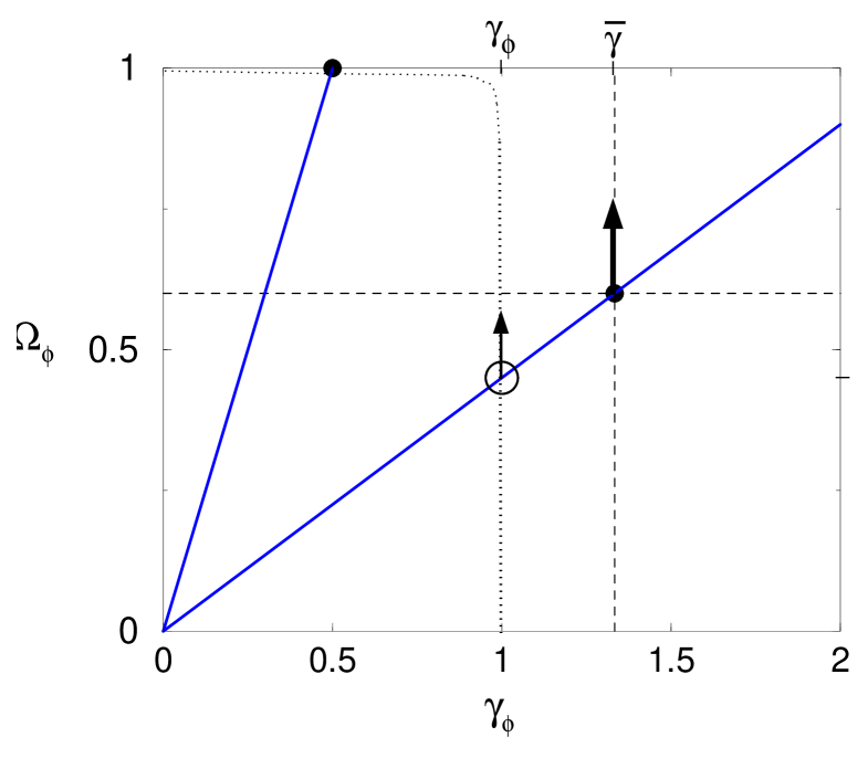
Figure 1: Schematic plot of the ’instantaneous fixed point’ (solid dot) and the the shadowing point (open circle), showing their movement in the $\left(\gamma_{\phi},\Omega_{\phi}\right)$ plane. For decreasing $\lambda_{i}$ ($\Gamma_{i}>1$), the instantaneous fixed point evolves to larger $\Omega_{\phi}$. The shadowing point shadows this point, riding on the $r=1$ line. It is at a smaller $\gamma_{\phi}$ such that it can stay on the $r=1$ line as it increases. Eventually $\lambda$ will decrease to the point where $\phi$ dominates ($\Omega_{\phi}\sim 1$).

III.2 Tracking in more general settings

In this section we extend the above analysis of tracking with a single scalar field and constant $\lambda$ to generalized settings with variable $\lambda_{i}$’s as well as

1. multiple tracking fields

2. scale-dependent potentials with $k_{i}\neq 0$

3. non-FLRW Hubble laws (expansion rate different from that of a FLRW universe)

As our interest is primarily in tracking quintessence models, the emphasis in the following discussion will be on the shadowing of attractor point $A$ in Table 1. As in the case of models with a single scalar field, one would expect a stable fixed point to still act as an instantaneous type attractor. When the $\lambda_{i}$’s are allowed to change slowly, the usual trajectories shadow these points. This shadowing amounts to the field being attracted to a surface, defined here by $r_{i}=1$. From the form of the equation of motion for $\widehat{\gamma}_{\phi i}$, it is easy to see that $r_{i}=1$ is an ‘attractor surface’ (for $\widehat{\gamma}_{\phi i}>\frac{k_{i}}{3}$, which we shall assume), which yields a fixed value of $\widehat{\gamma}_{\phi i}$. It is interesting to note that this $r_{i}=1$ condition is precisely equivalent to Eq. (10), although the latter was derived as a fixed point for a constant $\lambda_{i}$ case. We therefore focus on tracking that shadows point $A$ and maintains a constant equation of state (though in principle other forms of tracking may be possible) and take

$$r^{2}_{i}\equiv\frac{\lambda^{2}_{i}\Omega_{\phi i}}{3\left(\widehat{\gamma}_{\phi i}-\frac{k_{i}}{3}\right)\left(1-\frac{k_{i}}{6}\right)}=1$$ (18)

which ensures $\widehat{\gamma}_{\phi i}=const$ and in turn implies

$$\Omega_{\phi i}\cong\frac{3}{\lambda^{2}_{i}}\left(\widehat{\gamma}_{\phi i}-\frac{k_{i}}{3}\right)\left(1-\frac{k_{i}}{6}\right).$$ (19)

For the system of Eqs. (5) to close we also demand

$$\frac{d\ln\Omega_{\phi i}}{dN}\simeq-2\frac{d\ln\lambda_{i}}{dN}\Rightarrow-2\frac{d\ln\lambda_{i}}{dN}\simeq 3\left(\overline{\gamma}-\widehat{\gamma}_{\phi i}\right).$$

For a FLRW expansion rate, one has

$$\frac{d\kappa\phi_{i}}{dN}\simeq\frac{3}{\lambda_{i}}\left(\widehat{\gamma}_{\phi i}-\frac{k_{i}}{3}\right)$$ (20)

which gives

$$-2\frac{d\ln\lambda_{i}}{dN}\simeq-6\left(\widehat{\gamma}_{\phi i}-\frac{k_{i}}{3}\right)\left(1-\Gamma_{i}\right)\simeq 3\left(\overline{\gamma}-\widehat{\gamma}_{\phi i}\right)$$

which in turn yields an expression for $\widehat{\gamma}_{\phi i}$ in the form

$$\widehat{\gamma}_{\phi i}-\frac{k_{i}}{3}\simeq\frac{\overline{\gamma}-\frac{k_{i}}{3}}{2\Gamma_{i}-1}\simeq const.$$ (21)

Now for $\widehat{\gamma}_{\phi i}$ to be constant, as is required, either both $\overline{\gamma}$ and $\Gamma_{i}$ must be constants, or alternatively each needs to be arranged in such a way that the ratio appearing in (21) is constant. But in general there is no a-priori reason for the latter and we shall therefore not consider this possibility further. Since $\overline{\gamma}$ is the weighted average of all of the $\widehat{\gamma}_{\phi i}$, for tracking to occur for any field, we need either $\widehat{\gamma}_{\phi j}\simeq const\simeq\overline{\gamma}$ (which does admit the $\Omega_{\phi j}=1$ case) or $\Omega_{\phi j}\ll 1$. For quintessence, the first case can be consistent with the BBN bound of $\Omega_{\phi}\lesssim 0.15$ BBNBound (17). However, if one is considering tracking fields in other scenarios, such as during inflation, $\Omega_{\phi}\sim 1$ can also be acceptable.

We have given a schematic sketch of the tracking scenario in Figs. 1 and 2, corresponding to $k=0$ and $k>0$ respectively. In each case we have plotted both the instantaneous fixed point and the shadowing point depicted by a solid dot and an open circle respectively. Note that in each case the shadowing point falls on the $r=1$ line, but at a shifted $\gamma_{\phi}$, such that it can remain on the $r=1$ line, as the system ($\lambda$) evolves. Figure 2 illustrates the two significant effects of having $k>0$: the region $\widehat{\gamma}_{\phi}<k/3$ is excluded and the distance between the $\gamma_{\phi}$’s of the instantaneous fixed point and the shadowing point is narrower.

In the case of models with a generalized expansion rate (with $H_{gen}\neq H_{FLRW}$, as for example in models which include brane corrections or changes in the strength of gravity), the overall effect is to change the amount of friction the fields feel. More precisely, as was mentioned above, the form of the Eq. (3) implies that the attractor-type solutions exist as before, but their properties are determined by a new effective logarithmic slope $\widetilde{\lambda}_{i}$ defined by Eq. (4). The $i-th$ field will then instantaneously behave as if it had this effective logarithmic slope. However, the evolution of $\widetilde{\lambda}_{i}$ as a function of $N$ is not determined by rescaling $\lambda_{i}\left(N\right)$ by Eq. (4), since the $\lambda_{i}$ evolution equation does not transform in this way. As a result, when a correction to the expansion rate is present, the qualitative nature of the attractor can be understood from the value (or range of applicable values) of $\widetilde{\lambda}_{i}$. The robustness of tracking then depends on the nature of the modified attractor of the field $\phi_{i}$, which is determined by the value of $\widetilde{\lambda}_{i}$. Of course by the time of nucleosynthesis, $H_{gen}\simeq H_{FLRW}$, and the attractors will then be unmodified until the present time.

Whether a given modification to the expansion rate helps or harms tracking depends on the details of cosmological scenario in question. For example, a larger expansion rate in the early universe may cause an attractor to be at a smaller value of the field today where the slope of the potential is larger, and the field less able to dominate the energy content of the universe - or it may turn out that at a smaller field value the slope of the potential is less and thus the field is more likely to become dominant. Additionally, the transition from the non-FLRW attractor to the FLRW attractor may be abrupt, if the field can not shadow the attractor during the transition, in which case tracking can be disrupted. Thus, the effect of modifications to the Hubble law on the robustness of tracking depends on the details of the cosmological model - but given the necessary details, the effect can be determined by analyzing the attractors resulting from Eq. (4)

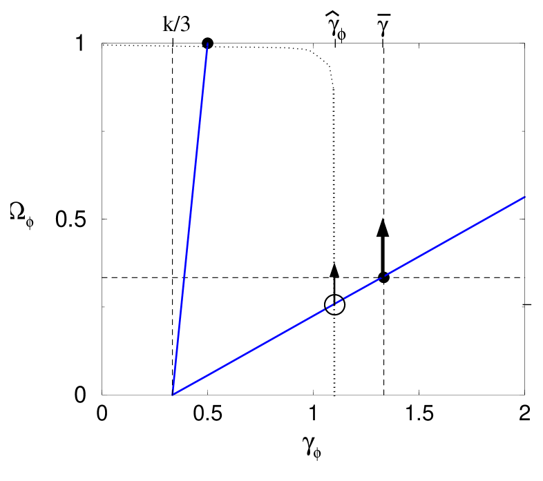
Figure 2: Schematic plot showing the effect of making the field’s potential scale factor dependent ($V\left(\phi,N\right)\propto\exp\left(-kN\right)$). The effect of $k>0$ is to set a minimum effective equation of state (that is, decay rate of $\rho_{\phi}$) for the field and to make it larger for the attracting point. Thus the shadowing point shadows the ’instantaneous fixed point’ more closely and comes to dominate more slowly. However, for $k\geq 3\overline{\gamma}$ tracking is impossible and the field dies away ($\Omega_{\phi}\rightarrow 0$). In this way $k$ can be said to act as a ’throttle’ for quintessence.

III.3 Tracking and independence from initial conditions

In general, the attractor of field $\phi_{j}$ is unique and independent of initial conditions. We will show this by constructing an equation involving $\phi_{j}$ and $\rho_{BG}$ as the only dynamical variables, which does not include the initial conditions of any of the fields $\phi_{j}$. One can then imagine solving this equation to obtain $\phi_{j}\left[\rho_{BG}\right]$, or equivalently, $\phi_{j}\left[N\right]$. In general one would expect this equation to possess a single, monotonically varying solution - although special cases where this is not the case can undoubtedly be constructed. The important point is that this solution is independent of the initial conditions of the fields.

To see this, the first step is to find $\overline{\gamma}$ as a function of the field values $\phi_{j}$. Using its definition and Eqs. (19) and (20) for each field, one can find a quadratic equation for $\overline{\gamma}$ as a function of $\lambda_{j}$, $\Gamma_{j}$, $k_{j}$ with $j=1,n$, in the form

$$\overline{\gamma}^{2}\left(\sum_{j}A_{j}\right)-\overline{\gamma}\left(1+\sum_{j}A_{j}\left(B_{j}+\frac{k_{j}}{3}\right)\right)+\left(\gamma_{BG}+\sum_{j}A_{j}B_{j}\frac{k_{j}}{3}\right)=0$$ (22)

where

$$\begin{array}[]{c}A_{j}\equiv\frac{3\left(1-\frac{k_{j}}{6}\right)}{\lambda_{j}^{2}\left(2\Gamma_{j}-1\right)^{2}}\\ B_{j}\equiv\left(2\Gamma_{j}-1\right)\left(\gamma_{BG}-\frac{k_{j}}{3}\right)+\frac{k_{j}}{3}.\end{array}$$ (23)

As this is a quadratic equation for $\overline{\gamma}\in\left[0,2\right]$, there may exist $0$, $1$, or $2$ solutions for $\overline{\gamma}$. The existence and stability of such solutions will be dealt with in the next section. The key point here is that solutions are manifestly independent of initial conditions. Combining Eqs. (19) and (20) yields

$$\Omega_{\phi i}=\left(\frac{3}{\lambda_{i}^{2}}\right)\frac{\left(1-\frac{k_{i}}{6}\right)\left(\overline{\gamma}-\frac{k_{i}}{3}\right)}{2\Gamma_{i}-1}=\Omega_{\phi i}\left[\phi_{k}\right]=\frac{1}{1+\frac{\rho_{BG}}{\rho_{\phi i}}}.$$ (24)

One can also write an expression for

$$\rho_{\phi i}=\frac{V}{1-\frac{1}{2}\gamma_{\phi i}}=\frac{V}{1-\frac{\overline{\gamma}-\frac{k_{i}}{3}}{2\left(2\Gamma_{i}-1\right)\left(1-\frac{k_{i}}{6}\right)}}=\rho_{\phi i}\left[\phi_{k}\right]$$ (25)

Thus one arrives at the following equation

$$\Omega_{\phi i}\left[\phi_{k}\right]=\frac{1}{1+\frac{\rho_{BG}}{\rho_{\phi i}\left[\phi_{k}\right]}}$$ (26)

This will generally be a very difficult expression to solve. However, it simplifies greatly when $\Omega_{\phi i}\ll 1$, because the fields are only coupled to each other through the effects each has on the Hubble expansion rate, and for $\Omega_{\phi i}\ll 1$ they effectively decouple, reducing the complexity of the system. In principal, the solution (if it exists, is physical, and is stable - issues we shall treat below) yields $\phi_{i}\left[N\right],\;\;i=1,n$, which are independent of initial conditions. Thus if the solution exists (i.e. is self-consistent) and is stable, then it is independent of the initial conditions.

The above argument depends on all of the fields being ’tracking fields’ - that is, Eqs. (19) and (20) being consistent with $r_{i}=1$ and thus $\widehat{\gamma}_{\phi i}=const$. Of course, not all the fields in a multi-field model need necessarily possess a potential that is compatible with tracking, in which case those fields would then not track. In such a case the argument given above for the independence from initial conditions is no longer valid. It is then impossible to make a general prediction about the existence or initial condition-independence of attractors for the tracking fields. However, as the fields affect one another through altering the background expansion rate (or altering the value and rate of change of $\overline{\gamma}$), one expects that if the $\Omega_{\phi i}$ of the non-tracking fields stay small, or if they do not cause $\overline{\gamma}$ to vary rapidly, they will not affect the attractor solution of the tracking fields, and leave intact the above result concerning independence from initial conditions, for the tracking fields.

IV Stability of tracking/shadowing solutions

We have shown above that the existence of instantaneous fixed points for the evolution equations (5) is mathematically consistent. However, for these points to give rise to tracking behavior they must also be attractors, that is, the shadowing point, determined by Eqs. (18) and (21) must be stable to perturbations. To find conditions for this, we shall obtain perturbation equations by perturbing the full evolution equations around the position of the shadowing point. From the nature of the eigenmodes of the perturbation equations the stability properties of the shadowing point can then be deduced. However, for models with $n$ fields, the problem of determining the perturbation eigenmodes becomes one of finding the eigenvalues for a $2n\times 2n$ matrix, or solving a polynomial of order $2n$. Fortunately, an exact solution is not necessary in order to address several important issues. These include the stability in the nearly decoupled limit ($\Omega_{\phi i}\ll 1$) and the determination of when the shadowing point will become unstable. Since the fields $\phi_{i}$ only affect each other through the expansion rate, one would expect that for small $\Omega_{\phi i}\ll 1$ the system will behave as $n$ decoupled systems, which turns out to be the case. The stability conditions for the decoupled fields correspond to the generalization of those found in LiddleTrack (14), with the added explicit scale dependence of the potential or corrections to the Hubble law taken into account. For the coupled case the results are also fairly intuitive: from the the shadowing conditions, one can see that $\widehat{\gamma}_{\phi i}$ should be nearly constant, and equal to a nearly constant multiple of the overall average equation of state $\overline{\gamma}$. Thus we have a key stability condition, namely that $\overline{\gamma}$ must be nearly constant. Now when $\Omega_{BG}$ dominates this condition is satisfied. However, if $\Omega_{\phi i}\left(\Gamma_{i}-1\right)$ become of order unity for any field $\phi_{i}$, even if each $\widehat{\gamma}_{\phi i}$ is constant, the proportion of the total energy density in the field increases rapidly, resulting in a rapid decease in $\overline{\gamma}$. Similarly, as $\sum_{j}\Omega_{\phi j}$ approaches unity, the condition $\overline{\gamma}=\gamma_{BG}\simeq const$ (and thus $\widehat{\gamma}_{\phi i}\simeq const$) can no longer be maintained. As one would expect, this manifests itself as a growing mode of the perturbations, which amounts to an instability. This disrupts tracking as $\sum_{j}\Omega_{\phi j}\rightarrow 1$. The important question is whether perturbations have growing modes if $\sum_{j}\Omega_{\phi j}<1$? In the next section we find that the answer to this question is negative, so long as $\overline{\gamma}$ and $\Gamma_{i}$ remain nearly constant.

IV.1 The perturbation equations

Assume for the moment that all fields are trackers - that is expressions (18) and (21) hold for each field individually. Now to study the perturbations, take

$$\begin{array}[]{ll}r_{i}-1=\epsilon_{i},&\;\;\;\;\;\left(2\Gamma_{i}-1\right)\left(\widehat{\gamma}_{\phi i}-\frac{k_{i}}{3}\right)=-\delta_{i}+\left(\overline{\gamma}-\frac{k_{i}}{3}\right)\end{array}$$ (27)

with the perturbations $\epsilon_{i},\delta_{i}\ll 1$. The resulting evolution equations for these perturbations become

$$\begin{array}[]{c}\frac{d\epsilon_{i}}{dN}=\frac{3}{2}\delta_{i}-3\epsilon_{i}\left(2+\overline{\gamma}\frac{2\Gamma_{i}-3}{2\Gamma_{i}-1}-4\frac{k_{i}}{3}\frac{\Gamma_{i}-1}{2\Gamma_{i}-1}\right)+\Delta\overline{\gamma}\\ \\ \frac{d\delta_{i}}{dN}=-\epsilon_{i}3\left(\overline{\gamma}-\frac{k_{i}}{3}\right)\left(\left(2-\frac{k_{i}}{3}\right)-\frac{\overline{\gamma}-\frac{k_{i}}{3}}{2\Gamma_{i}-1}\right)\\ +\frac{d\overline{\gamma}}{dN}-\frac{2\left(1-\delta_{i}\right)}{2\Gamma_{i}-1}\frac{d\Gamma_{i}}{dN},\end{array}$$ (28)

where the perturbation in $\overline{\gamma}$ due to the perturbation of each field is given by

$$\begin{array}[]{c}\Delta\overline{\gamma}\equiv\frac{3}{2}\sum_{j}\Omega_{\phi j}\left[\delta_{j}\left(\frac{\gamma_{BG}-\frac{k_{j}}{3}}{\overline{\gamma}-\frac{k_{j}}{3}}-\frac{2}{2\Gamma_{j}-1}\right)\right.\\ \left.-\epsilon_{j}2\left(\left(\gamma_{BG}-\frac{k_{j}}{3}\right)-\frac{\overline{\gamma}-\frac{k_{j}}{3}}{2\Gamma_{j}-1}\right)\right].\end{array}$$ (29)

This is the source of the coupling of the perturbations. Furthermore, the rate of change of $\overline{\gamma}$ enters into the perturbation equation, which is given by

$$\frac{d\overline{\gamma}}{dN}=\sum_{j}\Omega_{\phi j}\left[\left(\Gamma_{j}-1\right)6\left(\widehat{\gamma}_{\phi j}-\frac{k_{j}}{3}\right)\left(\widehat{\gamma}_{\phi j}-\gamma_{BG}\right)+\frac{d}{dN}\left(\widehat{\gamma}_{\phi j}-\gamma_{BG}\right)\right]+\frac{d\gamma_{BG}}{dN}.$$ (30)

Note that we are not presently taking $\gamma_{BG}$ to be a constant - the reason for which will become clear when we consider the effect on stability by non-tracking fields by absorbing them into a redefinition of the background. The condition for the closing of the unperturbed system of equations is that the terms in the stability equation above that are not proportional to $\epsilon_{j}$ or $\delta_{j}$ must vanish. Thus the following terms:

$$\sum_{j}\Omega_{\phi j}\left(\Gamma_{j}-1\right),\leavevmode\nobreak\ \leavevmode\nobreak\ \frac{d\ln\left(2\Gamma_{i}-1\right)}{d\kappa\phi_{i}},\leavevmode\nobreak\ \leavevmode\nobreak\ \frac{d\overline{\gamma}}{dN}$$ (31)

must be negligible compared to $\epsilon_{j}$ or $\delta_{j}$. For the $i-th$ field $\phi_{i}$ to have a stable $r_{i}=1$ tracking attractor, one requires that $\frac{d\ln\left(2\Gamma_{i}-1\right)}{d\kappa\phi_{i}}\ll 1\;$ for all $i$ as well as $\sum_{j}\Omega_{\phi j}\left(\Gamma_{j}-1\right)\ll 1$ and $\frac{d\gamma_{BG}}{dN}\ll 1$. That is, if the $\epsilon_{i}$ and $\delta_{i}$ equations without these terms are stable (have only decaying modes, with negative real parts of eigenvalues) then the $\epsilon_{i}$ and $\delta_{i}$ will decay until they are of the order of these ’residual’ quantities. Alternatively, one can say that the $r_{i}=1$ shadowing point is shifted by a small amount of the order these terms. Thus we proceed by assuming the terms that are not proportional to $\epsilon_{j}$ or $\delta_{j}$ are much smaller than $\epsilon_{j}$ and $\delta_{j}$, and analyze the resulting stability equation with these terms removed. This results in the following equations for $\epsilon_{i}$ and $\delta_{i}$

$$\begin{array}[]{c}\frac{d\epsilon_{i}}{dN}=\delta_{i}r+\epsilon_{i}a_{i}+\sum_{j}\epsilon_{j}b_{j}+\delta_{j}d_{j}\\ \frac{d\delta_{i}}{dN}=\epsilon_{i}c_{i}\end{array}$$ (32)

with

$$\begin{array}[]{c}a_{k}\equiv-\frac{3}{2}\left(2+\overline{\gamma}\frac{2\Gamma_{k}-3}{2\Gamma_{k}-1}-4\frac{k_{k}}{3}\frac{\Gamma_{k}-1}{2\Gamma_{k}-1}\right)\\ b_{k}\equiv-3\Omega_{\phi k}\left(\gamma_{BG}-\frac{k_{k}}{3}-\frac{\overline{\gamma}-\frac{k_{k}}{3}}{2\Gamma_{k}-1}\right)\\ c_{k}\equiv-3\left(\overline{\gamma}-\frac{k_{k}}{3}\right)\left(2-\frac{k_{k}}{3}-\frac{\overline{\gamma}-\frac{k_{k}}{3}}{2\Gamma_{k}-1}\right)\\ d_{k}\equiv-\frac{3}{2}\Omega_{\phi k}\left(\frac{2}{2\Gamma_{k}-1}-\frac{\gamma_{BG}-\frac{k_{k}}{3}}{\overline{\gamma}-\frac{k_{k}}{3}}\right)\end{array}$$ (33)

and

$$\Delta\overline{\gamma}=\sum_{j}\epsilon_{j}b_{j}+\delta_{j}d_{j}$$

In general, finding the eigenmodes of the above perturbation equations is equivalent to diagonalizing a $2n\times 2n$ matrix, or finding the roots of a polynomial of order $2n$ given by

$$1=\sum_{k}\frac{\beta b_{k}+d_{k}c_{k}}{\beta\left(\beta-a_{k}\right)-\frac{3}{2}c_{k}}.$$ (34)

Finding explicit expressions for the eigenmodes in terms of the coefficients (33) is neither feasible nor useful. Even for the simple 2-field case, one is faced with extremely messy expressions for the roots of a quartic equation. One, however, does not need to solve for all the $\beta$s explicitly. It is sufficient to impose the condition that the real parts of all relevant $\beta$s be negative. A mode is only relevant if its growth leads to the failure of tracking of the whole system. One would expect that some fields may not track, and at the same time not interfere with the tracking of other fields if they effectively decouple, having $\Omega_{\phi i}\ll 1$. In that case, these are irrelevant, or harmless instability modes. As a result, $Re\left[\beta\right]>0$ may not necessarily signal an instability in the entire tracking system, as the fields only interact by altering the value of $\overline{\gamma}$, and with $\Omega_{\phi i}\ll 1$ the failure of $\phi_{i}$ to track would not effect tracking by the other fields.

A possible way of studying the stability of the tracking is to recast the perturbation equations (32) into a system of equations analogous to $n$ coupled, damped harmonic oscillators ($\delta_{i}$) in the form

$$\frac{1}{\left(-c_{i}\right)}\frac{d^{2}\delta_{i}}{dN^{2}}+\frac{\left(-a_{i}\right)}{\left(-c_{i}\right)}\frac{d\delta_{i}}{dN}+\frac{3}{2}\delta_{i}=F\equiv-\sum_{j}\epsilon_{j}b_{j}+\delta_{j}d_{j}.$$ (35)

If one identifies $N$ with time, then the oscillator energy is a good measure of the deviation of the tracking fields from their shadowing condition (background) values. Thus there are $n$ oscillators $\delta_{i}$, each of which can be excited in $2n$ possible modes. Note that due to its form, equation (35) is not in general derivable from a conservative Lagrangian. In particular, note that the coefficients of the terms in $F$ proportional to $\delta_{j}$ do not in general form a symmetric matrix (and those proportional to $\epsilon_{j}$ an antisymmetric matrix), as would be necessary for $F$ to be derivable from an interaction potential of the form

$$F\neq\frac{d}{dN}\frac{\partial V}{\partial\dot{\delta}_{i}}-\frac{\partial V}{\partial\delta_{i}},\;\;\;\;V\equiv\sum_{j,k}C_{(jk)}\delta_{j}\delta_{k}+B_{\left[jk\right]}\delta_{j}\dot{\delta}_{k}$$

Thus the equations of motion do not conserve ’energy’ - that is, the perturbation amplitudes may decay or grow. However, by examining the implications of equation (35), one can determine what will happen - and thereby determine the stability of the system.

To do this, we shall employ the ansatz $\delta_{i}=\sum_{l}A_{il}e^{\beta_{l}N}$ and then solve mode-by-mode to obtain

$$\frac{A_{il}}{\left(-c_{i}\right)}\left[\beta^{2}_{l}-a_{i}\beta_{l}-\frac{3}{2}c_{i}\right]=F_{l}\equiv\sum_{j}\frac{A_{jl}}{\left(-c_{j}\right)}\left[d_{j}c_{j}+b_{j}\beta_{l}\right].$$ (36)

Because the right-hand side is independent of $i$, we can immediately determine the relative amplitudes for mode $l$ of oscillators $i$ and $k$:

$$\frac{A_{il}}{\left(-c_{i}\right)}\left[\beta^{2}_{l}-a_{i}\beta_{l}-\frac{3}{2}c_{i}\right]=F_{l}=\frac{A_{kl}}{\left(-c_{k}\right)}\left[\beta^{2}_{l}-a_{k}\beta_{l}-\frac{3}{2}c_{k}\right]\;\;\;\;\;\;i\neq k$$ (37)

We begin by examining the decoupled system ($F\rightarrow 0$). For the case of models with $n$ scalar fields, there are $2n$ eigenvalues $\beta^{0\pm}_{l}$, given by

$$\beta^{0\pm}_{l}=\frac{1}{2}\left(a_{l}\pm\sqrt{a^{2}_{l}+6c_{l}}\right).$$ (38)

From Eq. (37) it is clear that for the $\delta_{i}$ oscillator only the modes with frequencies $\beta^{0\pm}_{i}$ are present. The zeroth order stability condition is the requirement that $Re\left[\beta^{0\pm}_{i}\right]<0$. Using (38), this can be seen to be satisfied if and only if both $a_{i}<0$ and $c_{i}<0$. Solving these inequalities yields the following requirements for stability of uncoupled tracking

$$\begin{array}[]{ccc}&\frac{k_{i}}{3}<\overline{\gamma},&2\Gamma_{i}-1>\frac{2\left(\overline{\gamma}-\frac{k_{i}}{3}\right)}{2+\overline{\gamma}-2\frac{k_{i}}{3}}>0.\end{array}$$ (39)

Of course, for the zeroth order stability conditions to be relevant, we need $\sum_{j}\Omega_{\phi j}\left(\Gamma_{j}-1\right)\ll 1$ and $\sum_{j}\Omega_{\phi j}\ll 1$. Note that for $k_{i}=0$, the stability condition becomes $2\Gamma_{i}-1>\frac{2\overline{\gamma}}{2+\overline{\gamma}}$ or $\gamma_{\phi_{i}}<\frac{2+\overline{\gamma}}{2}$, which for $\overline{\gamma}\approx\gamma_{BG}$ agrees with that previously obtained in PJStrack (11) for the case of a single tracking field. This is not surprising, as in the decoupled limit of $\sum_{j}\Omega_{\phi j}\ll 1$ each field can be treated individually. This lower limit on $2\Gamma_{i}-1$ varies between $1$ and $\frac{1}{2}$, where $\Gamma_{i}=1$ is allowed unless $\overline{\gamma}=2$ and $\Gamma_{i}<1$ corresponds to a diminishing tracking field ($\frac{d\Omega_{\phi i}}{dN}<0$). For $\phi_{i}$ to be a “useful quintessence” field, that is to have $\frac{d\Omega_{\phi i}}{dN}>0$ ($\Gamma_{i}>1$), the condition (39) is automatically satisfied. For $k_{i}>0$ and $\Gamma_{i}>1$ tracking is still stable, and the lower limit on $2\Gamma_{i}-1$ becomes smaller, taking a value closer to $\frac{1}{2}$. One can understand this intuitively as follows: $k_{i}>0$ is another channel for the decay of (potential) energy in the field. Thus as less energy goes into kinetic energy, $\lambda_{i}$ changes less rapidly, and the system is more able to maintain the $r_{i}=1$ condition.

We now consider the effect of the coupling between the modes given by $F\neq 0$ in Eq. (36). The coupling causes the mixing of the modes, but diagonalizing the coupled system, as we have seen, is not practical. This is not necessary, however, as by examining the un-diagonalized system we can draw the important conclusion that the shadowing condition is stable until $\sum_{k}\Omega_{\phi k}\rightarrow 1$. From Eq. (37) it is clear that for each oscillator $\delta_{i}$, the modes with frequencies $\beta^{\pm}_{i}$ are dominant for $F\ll 1$, but there are now also $2\left(n-1\right)$ other modes present, with the frequencies of the other oscillators. The amplitudes of these other modes are suppressed by a factor of order $\sum_{k}\Omega_{\phi k}$ (unless $\beta^{0\pm}_{i}\simeq\beta^{0\pm}_{j}$, in which case $A_{ii}\sim A_{jj}$). One can see from Eq. (36) that the diagonal mode $A_{ii}$ can be treated as an oscillator, but with a shifted $mass^{2}$. We identify the zeroth order mode’s $mass^{2}$ with the $\frac{3}{2}\left(-c_{i}\right)>0$ term in Eq. (36). The effect of the interactions is then to provide a $mass^{2}$ shift of

$$\Delta m_{ii}^{2}=\sum_{j}\frac{\beta^{2}_{i}-a_{i}\beta_{i}-\frac{3}{2}c_{i}}{\beta^{2}_{i}-a_{j}\beta_{i}-\frac{3}{2}c_{j}}\left(-d_{j}c_{j}-b_{j}\beta_{i}\right).$$ (40)

The condition for stability then becomes the requirement that the shifted mass not cause the mode to become growing, which implies $Re\left[\beta_{i}\right]<0$. If $\Delta m_{ii}^{2}$ was real, then this would be the condition that the shifted $mass^{2}$ must be positive

$$m^{2}_{tot_{ii}}\equiv\frac{3}{2}\left(-c_{i}\right)+\Delta m_{ii}^{2}>0.$$ (41)

However, in general $\Delta m_{ii}^{2}$ is complex since $\beta_{j}$ are complex. The stability condition then becomes

$$Re\left[m^{2}_{tot_{ii}}\right]-\frac{1}{2}Im\left[m^{2}_{tot_{ii}}\right]^{2}>0.$$ (42)

This consideration does not significantly alter the story - that there is a stability radius of order unity around $m^{2}_{ii}=\frac{3}{2}\left(-c_{i}\right)$ in the complex plane. Thus in this way one can see that the system is guaranteed to be stable for any parameter values that ensure the inequality $\left|\Delta m_{ii}^{2}\right|<m_{ii}^{2}$ to be roughly satisfied.

Thus far we have been considering the diagonal elements of a mass matrix. We now consider the off-diagonal elements which correspond to the off-diagonal modes, whose amplitudes are controlled by Eq. (37). Until $\sum_{k}\Omega_{\phi k}\sim 1$, these off-diagonal mode amplitudes can not become of the same order of the diagonal mode amplitudes, and therefore Eq. (42) remains satisfied. We have seen that for $\sum_{j}\Omega_{\phi j}<1$ the diagonal mode amplitudes do not grow, and the off-diagonal mode amplitudes are suppressed relative to these by a factor of order $\sum_{k}\Omega_{\phi k}$. The implication is that the shadowing conditions (18) and (21) will be stable so long as $\sum_{j}\Omega_{\phi j}<1$.

The question remains as to what happens if some fields in the model are not trackers, and therefore do not satisfy the conditions (18) and (21)? These fields must then be excluded from the set of perturbations $\left\{\delta_{i},\epsilon_{i}\right\}$ and therefore do not contribute to $\Delta\overline{\gamma}$. Because they do not obey the tracking conditions, little can be said about such fields in general. They do, however, contribute to $\gamma_{BG}$. If their $\Omega$ is large enough such that they can cause an appreciable variation of $\overline{\gamma}$, they will cause a deviation from the shadowing conditions as noted above for the residual terms (31).

IV.2 Summary of stability conditions

We have shown that tracking with the $r_{i}=1$ condition is possible for nearly constant $\overline{\gamma}$. The constancy of $\overline{\gamma}$ is the key to closing the zeroth order tracking equations, and therefore it is not surprising that a constant $\overline{\gamma}$ is the key to the stability of the shadowing points, and that many of the stability conditions can ultimately be traced back to it. We note that even though in principle other forms of tracking may be possible under other conditions, the type of tracking considered here is that which has been commonly considered in the literature.

Note the near constancy of $\overline{\gamma}$ in turn requires nearly constant $\Gamma_{i}$ together with $\sum_{i}\Omega_{\phi i}\left(\Gamma_{i}-1\right)\ll 1$ and $\sum_{i}\Omega_{\phi i}<1$. We have seen that the perturbations $\epsilon_{i}$ and $\delta_{i}$ will decay until they are of order $\frac{d\ln\left(2\Gamma_{i}-1\right)}{d\kappa\phi_{i}}$, $\sum_{j}\Omega_{\phi j}\left(\Gamma_{j}-1\right)$ or $\frac{d\overline{\gamma}}{dN}$; resulting in the $r_{i}=1$ shadowing point to be shifted by small amount of the order of these terms. The system is more stable in the small $\Omega_{\phi i}$ limit, since as $\sum_{j}\Omega_{\phi j}\left(\Gamma_{j}-1\right)$ or $\sum_{j}\Omega_{\phi j}$ approach unity, this in general causes $\overline{\gamma}$ to vary rapidly, thus making the $r_{i}=1$ condition to fail and the tracking to cease. The weakly coupled case is analogous to $n$ individual tracking fields, and thus it is not surprising that the constraints in the limit of $k_{i}\rightarrow 0$ reproduce those given in PJStrack (11), for the single field case. Furthermore, in this limit $\overline{\gamma}\approx\gamma_{BG}$, and the stability of the shadowing condition for the field $\phi_{i}$, given by (18) and (21) require

$$\begin{array}[]{ccc}\frac{k_{i}}{3}<\overline{\gamma},&\;\;\;\;\;2\Gamma_{i}-1>\frac{2\left(\overline{\gamma}-\frac{k_{i}}{3}\right)}{2+\overline{\gamma}-2\frac{k_{i}}{3}}>0.\end{array}$$ (43)

If the stability conditions are not met for the field $\phi_{i}$, then clearly it will not track. However, the instability is irrelevant if $\Gamma_{i}<1$. This is because for $\Gamma_{i}<1$, the $\Omega_{\phi i}$ decreases with expansion (as $\widehat{\gamma}_{\phi i}>\overline{\gamma}$) and the field $\phi_{i}$ will effectively become irrelevant as $\Omega_{\phi i}\rightarrow 0$. Thus in this case the tracking of the other fields will not be effected by the failure of the field $\phi_{i}$ to track. On the other hand, if $\Gamma_{i}>1$, or if $\Gamma_{i}=1$ and $\Omega_{\phi i}$ is of order 1, then the instability in the field $\phi_{i}$ will ultimately ruin tracking for all fields, as it will cause $\overline{\gamma}$ to vary rapidly, and $r_{i}=1$ can no longer be maintained in general for any of the other fields. Finally, we have seen that the presence of non-tracking fields will harm tracking if and only if they cause $\overline{\gamma}$ to vary rapidly.

We note that our stability analysis was limited to the violation of the shadowing conditions given by (18) and (21). A concern that we have not addressed is the possibility that the homogeneous distribution of the scalar field may be unstable to formation of spatial inhomogeneities - the so called ’Q-balls’ Qball_Paper (18). This is an important issue that we hope to return to in future work.

V Conclusions

We have argued that for tracking quintessence to truly solve the fine-tuning problem, the tracking phenomena must be robust in the more complicated and complete cosmological scenarios that derive from high energy physics. Such scenarios typically include multiple scalar fields (some of which may not have potentials suitable for tracking), a Hubble law at high energies different from that of the FLRW model, and scalar field potentials that depend explicitly on the scale factor. Tracking would be of limited use as a solution to the fine-tuning problem if it were easily ruined by such effects.

In models with $n$ scalar fields, we have found that $r_{i}=1$ tracking requires a nearly constant $\overline{\gamma}$. If any one of the tracking fields develops a large enough $\Omega_{\phi i}\left(\Gamma_{i}-1\right)$, or if $\sum_{j}\Omega_{\phi j}\rightarrow 1$ then in general $\overline{\gamma}$ will vary rapidly, causing the tracking to fail for all fields. Also, if any of the non-tracking fields become a significant portion of the total energy density then they can potentially cause $\overline{\gamma}$ to vary rapidly. In general, therefore, $r_{i}=1$ tracking requires $\Gamma_{i}$ to be nearly constant for the field $\phi_{i}$ to track, as well as $\Omega_{\phi i}\left(\Gamma_{i}-1\right)\ll 1$ for all fields, and for $\sum_{j}\Omega_{\phi j}$ not to approach $1$.

In models with a modified expansion rate (such as those including the brane corrections or changes in the strength of gravity), we have found the attractor-type solutions can still exist, but their instantaneous nature is determined by the effective logarithmic slope $\widetilde{\lambda}_{i}$. When such a correction is present, the qualitative nature of the attractor can be understood from the value of $\widetilde{\lambda}_{i}$. However, the answer to the question of whether a given modification to the expansion rate helps or harms the robustness of tracking depends on the details of cosmological scenario in question - but given the necessary details, the effect can be determined by analyzing the attractors resulting from Eq. (4).

In models with temperature dependent potentials ($k_{i}>0$), we have found that this dependence can make tracking more robust. Roughly speaking, $k_{i}>0$ ’throttles’ quintessence - slowing the rate of increase of $\Omega_{\phi i}$, thus making fields with larger $\Gamma_{i}$ less harmful to both tracking stability, and to cosmological scenarios. On the other hand, very large values of $k_{i}$ spoil tracking for field $\phi_{i}$. If $\Gamma_{i}>1$, a value of $0<k_{i}<3\overline{\gamma}$ keeps ($\overline{\gamma}-\widehat{\gamma}_{\phi i}$) small, and slows the increase of $\Omega_{\phi i}$, making tracking of the entire system more stable. For $k_{i}\geq 3\overline{\gamma}$ the field $\phi_{i}$ will fail to track, though it becomes an irrelevant field and tracking of the other fields is not harmed.

In conclusion, we have found that the conditions for robustness of tracking becomes more complex in the more general settings that derive from high energy physics. Tracking can become more fragile with respect to some such added complexities to the model, as there are more constraints to be satisfied. This can for example be seen from the above analysis of stability in presence of multiple scalar fields. Other additions, such as temperature dependent potentials, on the other hand may make tracking more robust. Interestingly though, most of the cases where tracking is disrupted are those in which the cosmological model is itself non-viable due to other constraints. For example, although tracking is less robust for larger $\sum_{j}\Omega_{\phi j}$, this would generally make the model non-viable due to constraints such as nucleosynthesis and structure formation. Thus tracking seems to fair well in these general settings, once we confine ourselves to viable cosmological models.

References

- (1) A. Miller et al., astro-ph/0108030
-
(2)
P.D. Mauskopf et al., ApJ. 536 L59-L62, 2000
A.E. Lange et. al., Phys. Rev. D64 042001, 2001 -
(3)
A. T. Lee at al., Proceedings 3K Cosmology, 1998
T. Padmanabhan and Shiv K. Sethi, astro-ph/0010309 -
(4)
N.A. Bahcall and X. Fan, Aptrophys. J. 504 1, 1998
N.A. Bahcall, X. Fan and R. Cen, ApJ 485 L53, 1997
R.G. Carlberg, S.M. Morris, H.K.C. Yee, E. Ellingson, Aptrophys. J. 479 L19, 1997 -
(5)
L.N. da Costa et al., MNRAS 299 425, 1998
M. Davis, A. Nusser and J. Willick, Aptrophys. J. 473 22, 1993
J. Willick and M. Strauss, Aptrophys. J. 507 64, 1998
J. Willick et al., Aptrophys. J. 486 629, 1997 -
(6)
A.E. Evrard, MNRAS 292 289, 1997
L. Lubin et al., Aptrophys. J. 460 10, 1996
L.N. da Costa et al., MNRAS 299 425, 1998
M. Davis, A. Nusser and J. Willick, Aptrophys. J. 473 22, 1993
J. Willick and M. Strauss, Aptrophys. J. 507 64, 1998
J. Willick et al., Aptrophys. J. 486 629, 1997 - (7) Limin Wang, R.R. Caldwell, J.P. Ostriker and P.J. Steinhardt, Aptrophys. J. 530 17, 2000, and references therein
-
(8)
Perlmutter et al., Aptrophys. J. 483 565, 1997
B.P. Schmidt et al., Aptrophys. J. 507 46, 1998
A.G. Riess et al., Astron. J. 116 1009, 1998
S. Perlmutter et al., Astrophys. J. 517 565, 1999 - (9) R.R. Caldwell, R. Dave and P.J. Steinhardt, Phys. Rev. Lett. 80 1582-1585, 1998
- (10) B. Ratra and P.J.E. Peebles, Phys. Rev. D37 3406, 1998
- (11) P.J. Steinhardt, Limin Wang and Ivaylo Zlatev, Phys. Rev. D59 123504, 1999
-
(12)
P. Binetruy, C. Deffayet, U. Ellwanger, and D. Langlois, Nucl. Phys.
B565 269, 2000
P. Binetruy, C. Deffayet, U. Ellwanger, and D. Langlois, Phys. Lett. B477 285, 2000
P. Kraus, JHEP 9912 011, 1999
E.E. Flanagan, S.-H.H. Tye, and I. Wasserman, Phys. Rev. D62 044039, 2000
T. Shiromizo, K. Maeda, and M. Sasaki, Phys. Rev. D62 024012, 2000 - (13) S. Mizuno, Kei-ichi Maeda, hep-ph/0108012
- (14) E. Copeland, A. Liddle and D. Wands, Phys. Rev. D57 4686-4690, 1998
- (15) G. Huey and J.E. Lidsey, Phys. Lett. B514 217-225, 2001
- (16) A.R. Liddle, A. Mazumdar and F.E. Schunck, Phys. Rev. D58 06130, 1998
- (17) P. G. Ferreira and M. Joyce, Phys. Rev. Lett. 79 4740, 1997; Phys. Rev. D 58 023503, 1998
- (18) S. Kasuya, astro-ph/0105408