Exo-planet detection with the COROT space mission.
I. A multi-transit detection criterion.

Abstract

In this note, we present a detection criterion for exo-planets to be used with the space mission COROT. This criterion is based on the transit method that suggests to look for stars dimming caused by partial occultations by planetary companions. When at least three transits are observed, we show that a cross-correlation technique can yield a detection threshold, thus enabling to evaluate the number of possible detections assuming a model for the stellar population in the Galaxy.

1 Overview of COROT

1.1 Introduction

Exo-planets detection has now become a very active field in astrophysics. In august 2000, about fifty Jupiter-like planets have been discovered around nearby stars. The next challenging step is to find much less massive planets with the hope to detect life on some of them afterwards. COROT, a CNES space mission to be launched in 2004 [1], is currently a funded project capable of detecting planets with a radius close to $1\,R_{\oplus}$ thanks to the “transit method” [2]. In this section, we briefly describe the transit method and the COROT satellite. In section 2, we present a detection criterion for multi-transits, and in section 3, we discuss the number of possible dectections assuming a model for the stellar population in the Galaxy. The specific case of mono-transits will be considered in a forthcoming article.

1.2 The transit method

The transit method for searching extrasolar planets is based on the idea that if a planet crosses the disk of its parent star, it would result in a dimming of the star’s observed light [3-4]. The expected amplitude of the relative stellar flux dimming is:

$$\varepsilon\equiv\frac{\Delta F}{F}={\left(\frac{R_{P}}{R_{\star}}\right)}^{2}$$ (1)

where $F$ is the flux, $R_{P}$ the radius of the planet and $R_{\star}$ the radius of the parent star. We call impact parameter, expressed in stellar radii, the apparent height of the planet trajectory above the star’s equator. For an impact parameter equal to 0.5, the transit duration is:

$$tr=\frac{\sqrt{3}\,R_{\star}}{\sqrt{GM_{\star}}}\,\sqrt{a}$$ (2)

where $a$ is the orbital radius. This duration is respectively 11.2 and 25.7 hours for the Earth and Jupiter in the solar system, and 3 hours for 51 Peg b [5]. The geometrical probability that the orbital inclination on the sky is close enough to 90^o to make a transit visible is:

$$p_{g}=\frac{R_{\star}}{a}$$ (3)

$p_{g}$ equals to 0.5% for the Earth, 0.1% for Jupiter and 16% for 51 Peg b. This method has already been succesfully used from ground and space on the planetary companion of HD209458, previously detected by radial velocity techniques, e.g. [6].

1.3 Focusing on multi-transits

COROT features a 27 cm telescope and four $2048\times 2048$ CCDs, two of which are devoted to the exoplanets program. During its 2.5-year mission, the satellite will monitor 5 fields of 5000 to 12000 stars (${11\leq m_{V}\leq 16.5}$, galactic latitude $=15-20^{\circ}$), each of them for 150 days, thus leading up to 60000 lightcurves. The task will be then to look in the data for the signatures of planetary transits. In order to estimate the number of potential detections by COROT, we propose to consider here a rather basic method based on a cross-correlation technique. More accurate techniques are under study at the Laboratoire d’Astronomie Spatial in Marseille [7], or have been already suggested [8]. Here we will consider only multi-transits, which means that a given planet will have to transit at least 3 times in front of its parent star to be detected by this method. The sought after signal looks like a repeated dimming in the parent star lightcurve, at even time intervals corresponding to the planetary orbital period $P$.

2 Principle of data processing

2.1 Raw data averaging

To increase the signal to noise ratio (SNR) and also to reduce the amount of data, we begin by averaging the raw data, i.e. samples of the total flux $F$ every 16 minutes over 150 days, on the duration of a presumed transit $tr$ (up to 15 hrs). This operation leads to a ${N=150\times 24/tr}$ point vector in which a potential event is reduced to one point. It means that in the whole process of the transit search, all relevant values of $tr$ should be tried.

2.2 Transit signal modelling

The transit signal $s$ we are looking for can be modeled by the sum of a Dirac comb $\alpha\,\Pi_{k}$ (k teeth, amplitude $\alpha$) and a gaussian white noise $b$ of standard deviation $\sigma_{b}$:

$$\forall i\in\{1,...,N\}\,,\quad s[i] = -\alpha\,\Pi_{k}[i]+b[i]$$ (4)

$$\mbox{where}\quad\Pi_{k}[i] = \sum_{m=0}^{k-1}\delta[i-m\frac{N}{k}]$$ (5)

($\delta$ is Kroenecker’s symbol). The term $b$ is the sum of several types of noises:

• the photon noise: $\sigma_{ph}=\sqrt{N_{ph}}$ ($N_{ph}$ refers actually to the number of stellar photo-electrons detected by the detector during $tr$)

• the electronical read-out noise: $\sigma_{ro}=12\,e^{-}.pixel^{-1}$

• the background noise (essentially zodiacal light): $\sigma_{bg}=16\,e^{-}.pixel^{-1}$ (exposure time is 32 s)

• the stellar irradiance variability noise depending on the averaging interval whose length is $tr$: $\sigma_{st}(tr)=N_{ph}(tr)\,\sigma_{st}(tr)_{ppm}$. For G and K stars, an estimated value of this quantity can be obtained through filtering of the SOHO-VIRGO data acquired on the Sun [9]: $\sigma_{st}(tr)_{ppm}\sim 30-75\,ppm$ for $tr=2-15\,hrs$.

• the noise introduced by random pointing error of the satellite is supposed to be perfectly corrected by onboard processing

For simplicity, all those noises are supposed independant, white and gaussian noises. Consequently, we get:

$$\sigma_{b}=\sqrt{N_{ph}+n\,(\sigma_{ro}^{2}+\sigma_{bg}^{2})+\sigma_{st}^{2}}$$ (6)

where $n$ denotes the total number of read-out pixels during the transit.

2.3 Detection with cross-correlation

The idea is to compute cross-correlation products between the data and a Dirac comb (amplitude unity) which has the shape of a noise free multi-transit signal (see fig.1). For a given value of $k$, we get $N/k$ products of this kind, denoted $C_{k}$:

$$C_{k}=\frac{1}{N}\sum_{i=0}^{N-1}s[i]\,\Pi_{k}[i]=\frac{1}{N}\left[\alpha\,k+\sum_{m=0}^{k-1}b[m\frac{N}{k}]\right]$$ (7)

Trying all values of k between 3 and 50 (${3\leq P\leq 50\,\mbox{days}}$) means computing ${\sum_{k=3}^{50}N/k=\gamma N}$ products (${\gamma\simeq 3.0}$). The presence of a transit must be somehow related to a high value of $C_{k}$, but the question is: where to draw the line?

2.4 Statistical analysis

The answer to this question lies in a statistical analysis of the problem. To begin with, let us consider the set of $N/k$ products $C_{k}$ for a given $k$. $C_{k}$ can be seen as a random variable. Because we assumed that $b$ is a gaussian noise with a null mean and a standard deviation $\sigma_{b}$, the probability law of $C_{k}$ should also be gaussian with a standard deviation ${\sigma_{C}=\sqrt{k}\sigma_{b}/N}$. Its mean value should be equal to $\alpha k/N$ in case of a star actually showing transits or zero otherwise. Let $p_{k}$ be the probability of having ${C_{k}\leq\beta_{k}\,\sigma_{C}}$ in case of noise only (no transit):

$$p_{k}=Pr\{C_{k}\leq\beta_{k}\sigma_{C}\}=\frac{1}{2}\left[1+\mbox{erf}\left(\frac{\beta_{k}}{\sqrt{2}}\right)\right]$$ (8)

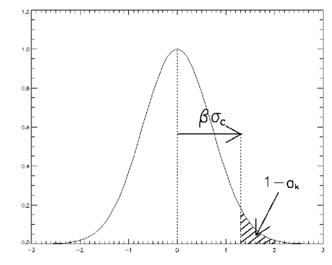
Figure 1: Raw data are averaged on the duration of the presumed transit, then cross-correlated with a Dirac Comb.

Figure 2: The probability distribution of the cross-correlation products $C_{k}$ is centered around zero, because the absence of a transit is the general rule. A large value of a $C_{k}$ with respect to $\sigma_{C}$ is indicative of a transit with a level of confidence $a_{k}$. This confidence is also measured by $\beta$, which is supposed common to all $k$.

The probability that all the $N/k$ values of $C_{k}$ will remain inferior to $\beta_{k}\sigma_{C}$ is ${a_{k}=p_{k}^{N/k}}$. This gives the level of confidence that the statistical noise would not generate a high value of $C_{k}$ that would be mistaken for a transit (see fig.2). If the statistics bear on all values of $k$ ($\gamma N$ cross-correlation products), the level of confidence becomes:

$$a=\prod_{k=3}^{50}a_{k}=\prod_{k=3}^{50}{\left\{\frac{1}{2}\left[1+\mbox{erf}\left(\frac{\beta_{k}}{\sqrt{2}}\right)\right]\right\}}^{N/k}$$ (9)

One can numerically show that $\beta$ depends weakly on $k$ provided $a$ is close enough to one (no more than 10% variations). That is why we will assume that $\beta$ is common to all $k$, in order to solve for $\beta$, given the global level of confidence $a$:

$$\mbox{erf}\left(\frac{\beta}{\sqrt{2}}\right)+1-2a^{\frac{1}{\gamma N}}=0$$ (10)

For example, the transit of a planet orbiting a sun-like star at 0.05 AU (such as 51 Peg b) would last approximately 3 hrs if the line of sight belongs to the orbital plane. In this case $N=1200$, and solving (10) for $a=99.9\,\%$ leads to $\beta=5.0$ (see fig.3).

2.5 SNR detection criterion

Assume that a global level of confidence $a$ has been chosen and has yielded up a value of $\beta$: a detection could be claimed with that confidence, if among the $\gamma N$ cross-correlation products, one is greater than $\beta\,\sigma_{C}$. As it is a signature of a transit, its value can be written as $\alpha k/N$, so the detection criterion translates into the inequation:

$$\frac{\alpha\,k}{N}\geq\frac{\sqrt{k}\,\beta\,\sigma_{b}}{N}$$ (11)

Introducing the SNR on a single event (a single dimming of the lightcurve) defined by $S/N=\alpha/\sigma_{b}$, we get:

$$\frac{S}{N}\geq\frac{\beta}{\sqrt{k}}$$ (12)

As expected, the required SNR increases with the level of confidence and decreases with the number of observed transits. To go on with the previous example, $P=4.1\,\mbox{days}$ so $k=36$ and ${S/N\geq 0.7}$ ! As we see here, this cross-correlation technique is enough powerful to detect repetitive transits with lower than unity SNR on single events.

2.6 Link with the planetary radius

The amplitude of the relative dimming of the parent star lightcurve is connected to the radius of the transiting planet $R_{P}$ by:

$$\frac{\Delta F}{F} = {\left(\frac{R_{P}}{R_{\star}}\right)}^{2}$$ (13)

$$\mbox{besides}\quad\frac{\Delta F}{F} = -\frac{\alpha}{N_{ph}}\;=\;-\frac{S}{N}\frac{\sigma_{b}}{N_{ph}}$$ (14)

Thus (12) translates into:

$$R_{P}\geq R_{\star}\,{\left(\frac{\beta}{\sqrt{k}}\frac{\sigma_{b}}{N_{ph}}\right)}^{\frac{1}{2}}$$ (15)

which gives the minimum planetary radius that can be detected with a level of confidence $a$. In our example, if we assume for the star $m_{V}=14$ and given the characteristics of COROT, we compute: $R_{P}\geq 1.5\,R_{\oplus}$.

3 Expected number of detections

3.1 Assumptions

To have a realistic distribution of stars per spectral type and magnitude interval in the observed fields, we have used a model of the stellar population in the Galaxy developped at Besançon Observatory [10]. Only stars on the Main Sequence have been considered (type V stars). We will assume that every observed star has 100% probability of having a planet orbiting at the distance tested, and that orbits are circular. For every distance, we compute the minimum radius the planet should have for our criterion to be able to detect it with a false alarm level of $10^{-5}$.

3.2 Algorithm

Let $a$ be the orbital of the planetary orbit. We define the reduced orbital radius by ${a_{r}=a{(L_{\star}/L_{\odot})}^{-0.5}}$ so that $a_{r}=1$ AU would always correspond to the distance where the planet receives as much flux from its parent star as the Earth from the Sun. Computations have been done in the range $a_{r}=0.03-1$ AU.

Given the star characteristics: mass $M_{\star}$, radius $R_{\star}$, effective temperature $T_{\star}$, luminosity $L_{\star}$, spectral type $Sp$ and magnitude $m_{V}$, we compute:

• the orbital radius $a$ in AU;

• the revolution period $P$ in days;

• the probability of seeing 3 transits in 150 days: $p_{g}\times\frac{150}{P}$ ($P\leq 50$ d);

• the transit duration $tr$ (assuming a mean impact parameter of 0.5);

• the number of photo-electrons $N_{ph}$ received during $tr$.

Then, the SNR detection criterion imposes a minimum value for the signal $\varepsilon=(S/N)/\sqrt{N_{ph}}$, and consequently for the detectable planetary radius $R_{P}=R_{\star}\,\sqrt{\varepsilon}$.

3.3 Results

We have plotted the number of detections as a function of the reduced orbital distance for various planetary radii (fig.4) and for a false alarm rate of $10^{-5}$. For every curve, it is the minimum detectable radius (expressed in Earth unit) that is considered. Results are given for the whole mission. This way of presenting our results was chosen because of the unknown frequency of the different planetary types. Anyone can apply to our curves the scaling factor of his choice. For instance, assuming a 2% probability of existence, COROT could detect several tens of “hot Jupiters” enhancing significantly the statistics on this class of planets. What is more, COROT has the potential to spot “hot Earths” if any, since for example around 4 events would be expected if 20% of the stars exhibit earth planets at 0.05 AU.

4 References

[1] Baglin A. et al., Asteroseismology from space - The COROT experiment, New Eyes to See Inside the Sun and Stars, IAU 185 (1998) 301.

[2] Rouan et al., Searching for exosolar planets with the COROT space mission, Physics and Chemistry of the Earth Part C, v. 24, iss. 5 (1999) 567-571.

[3] Rosenblatt F., A two-color photometric method for detection of extra-solar planetary systems, Icarus, 14 (1971) 71-93.

[4] Schneider J., Extra-solar planets transits: detection and follow up, VLT Opening Symposium Antofagasta, Springer, 1999.

[5] Mayor M., Queloz D., A Jupiter-mass companion to a solar-type star, Nature, 378 (1995) 355-359.

[6] Charbonneau et al., Detection of Planetary Transits Across a Sun-like Star, ApJ, 529 (2000) L45-L48.

[7] Defaÿ C. et al., A bayesian method for the detection of planetary transits, submitted to A&A (2000).

[8] Jenkins et al., A Matched Filter Method for Ground-Based Sub-Noise Detection of Terrestrial Extrasolar Planets in Eclipsing Binaries: Application to CM Draconis, Icarus, 119 (1996) 244-260.

[9] Fröhlich et al., First results from VIRGO, the experiment for helioseismology and irradiance monitoring on SOHO, Solar Physics, 170 (1997) 1-25.

[10] Robin A., Crézé M., Stellar population in the Milky Way - A synthetic model, A&A, 157 (1986) 71-90.

Figure 3: $\beta$ as a function of the false alarm percentage $1-a$. This quasi logarithmic relation allows to get high confidence levels with reasonable SNR.

Figure 4: This plot shows the number of expected detections during the full life-time of the mission, provided 100% of the stars have a planetary companion of radius $R_{P}$ at the distance $a_{r}$, and assuming a false alarm rate of $10^{-5}$. The number attached to each curve is the minimum value of $R_{P}$ (expressed in Earth unit) enabling the detection.